Simplifying a hydrological ensemble prediction system with a backward greedy selection of members – Part 1: Optimization criteria

(1)

www.hydrol-earth-syst-sci.net/15/3307/2011/ doi:10.5194/hess-15-3307-2011

Earth System

Sciences

Simplifying a hydrological ensemble prediction system with a

backward greedy selection of members – Part 1: Optimization

criteria

D. Brochero1,2, F. Anctil1, and C. Gagn´e2

1_{Chaire de recherche EDS en pr´evisions et actions hydrologiques, Department of Civil Engineering and Water Engineering,}

Universit´e Laval, Qu´ebec, G1V 0A6, Canada

2_{Computer Vision and Systems Laboratory (CVSL), Department of Electrical Engineering and Computer Engineering,}

Universit´e Laval, Qu´ebec, G1V 0A6, Canada

Received: 21 February 2011 – Published in Hydrol. Earth Syst. Sci. Discuss.: 11 March 2011 Revised: 14 September 2011 – Accepted: 10 October 2011 – Published: 4 November 2011

Abstract. Hydrological Ensemble Prediction Systems (HEPS), obtained by forcing rainfall-runoff models with Meteorological Ensemble Prediction Systems (MEPS), have been recognized as useful approaches to quantify uncer-tainties of hydrological forecasting systems. This task is complex both in terms of the coupling of information and computational time, which may create an operational bar-rier. The main objective of the current work is to assess the degree of simplification (reduction of the number of hydrological members) that can be achieved with a HEPS configured using 16 lumped hydrological models driven by the 50 weather ensemble forecasts from the European Cen-tre for Medium-range Weather Forecasts (ECMWF). Here, Backward Greedy Selection (BGS) is proposed to assess the weight that each model must represent within a subset that offers similar or better performance than a reference set of 800 hydrological members. These hydrological mod-els’ weights represent the participation of each hydrologi-cal model within a simplified HEPS which would issue real-time forecasts in a relatively short computational real-time. The methodology uses a variation of thek-fold cross-validation, allowing an optimal use of the information, and employs a multi-criterion framework that represents the combination of resolution, reliability, consistency, and diversity. Results show that the degree of reduction of members can be estab-lished in terms of maximum number of members required (complexity of the HEPS) or the maximization of the rela-tionship between the different scores (performance).

Correspondence to:D. Brochero ([email protected])

1 Introduction

In hydrology, as in many applications, it is accepted that there is no superior model for every application under all circum-stances (Duan et al., 2007; Alpaydin, 2010). Today, the avail-ability of the Meteorological Ensemble Prediction Systems (MEPS) and its subsequent coupling with multiple hydro-logical models offers the possibility of building Hydrologi-cal Ensemble Prediction Systems (HEPS) relying on a large number of members. But the complexity of such HEPS be-comes an operational burden when one has to evaluate sev-eral hundreds of scenarios at each time step.

To provide an idea of the complexity that can be achieved in HEPS, represented for example by the number of members to handle, it is worth mentioning the principal areas of un-certainty associated with the hydrological process (Schaake et al., 2007) as follows:

– Uncertainty from the meteorological data: in this case, the MEPS are responsible for providing this informa-tion. Different centres around the world are currently working on this issue, for example the TIGGE initia-tive consists of ensemble forecast data from ten global centres, for a total of 259 members (TIGGE, Bougeault et al., 2010). In relation to this, Bao et al. (2011) have shown that a HEPS comprised of meteorological mem-bers derived from multiple meteorological centres may actually perform better as compared to an ensemble de-rived from a single meteorological model.

(2)

process: the initialization uncertainty (i.e. the initial state of the model) and the model uncertainty (from pa-rameter identification to model conceptualization). In this regard, the methodology proposed by Beven and Binley (1992) provides the evaluation of parameter un-certainty from the point of view of equifinality. For ex-ample Pappenberger et al. (2005) have shown the advan-tages in HEPS to flood inundation predictions coupling MEPS with both hydrological and hydraulic models that have been evaluated at the same time with the GLUE methodology.

Another way of conceptualizing the uncertainty of the model focuses on a multi-model approach, making good use of the resources invested in the development of dozens of hydrological models. For instance, Vel´azquez et al. (2011) have shown, based on the database of the present paper, that the ensemble predictions produced by a combination of several hydrological model structures and meteorologi-cal ensembles have higher skill and reliability than ensemble predictions given either by a single hydrological model fed by weather ensemble predictions or by several hydrological models driven by a deterministic meteorological forecast.

Cloke and Pappenberger (2009) have already highlighted the computational demand of using MEPS for flood forecast-ing as one of the main points to overcome in the future, either by new technologies (stochastic chip technology) or by effi-cient use of computing clusters. Thus, the selection of hydro-logical members as part of a simplified model can be useful given the computational cost of running models and creating ensembles. Vrugt et al. (2008) have suggested the selection of hydrological models as an additional task that can be run based on the results of the post-processing using Bayesian Model Averaging (BMA) in a multi-criteria framework.

As a compromise, researchers have attempted to cluster MEPS for flood prediction in various ways: by lagging en-sembles and deriving representative members through hier-archical clustering over the domain of interest, and thus to produce a reduced ensemble set at higher resolution (Mar-sigli et al., 2001); by analyzing the relation between atmo-spheric circulation patterns and extreme discharges (Ebert et al., 2007), or by establishing, in a deterministic way (“best match” approach), the location of the forecast that is the most similar to the rainfall pattern of the catchment (Xuan et al., 2009).

Here, we propose the selection of hydrological mem-bers directly in the HEPS with a technique called Back-ward Greedy Selection under the different scores presented in Sect. 2. In the case of MEPS with interchangeable mem-bers (the case presented here), the selection is oriented to evaluate the hydrological models participation inside a sub-set of a few members.

The HEPS under study is formed of 16 lumped hydrolog-ical models forced by the 50 meteorologhydrolog-ical inputs of the ECWMF EPS, leading to a grand-ensemble of 800 members.

This approach was tested in 10 catchments located in France for a period of seventeen months (from March 2005 to July 2006). Another important feature of the HEPS at hand is the short duration of the series. This has been highlighted by several authors as a negative point in the evaluation of system performance in the case of extreme events (Renner et al., 2009; Cloke and Pappenberger, 2009). This condition imposes the use of resampling and recombination techniques in the proposed methodology shown in Sect. 3.

Other studies that focused on periods of analysis very sim-ilar to the one used in this paper have also proven the useful-ness of the ECMWF EPS. For example Rousset et al. (2007) evaluated hundreds of French catchments from 4 Septem-ber 2004 to 31 July 2005 showing that the information given by the ensemble forecast is useful for flood warning and water management agencies. Similarly, Thirel et al. (2008), in a comparative analysis of short-range meteoro-logical forecasts from the ECMWF EPS and PEARP EPS of M´et´eo-France under the scheme of SIM coupling, anal-ysed the competence jurisdiction of each of the two EPS from 11 March 2005 to 30 September 2006, showing that the ECMWF EPS seemed best suited for low flows and large basins while the PEARP EPS was best suited for floods and small basins.

We do emphasize that the results shown in this first phase focused primarily on the analysis of the scores in the process of selecting hydrological members. Furthermore, we evalu-ated the notion of interchangeability of the MEPS and HEPS members, concluding that the participation of the hydrologi-cal models in the subset of selected members is sufficient to guide the members’ selection, as shown below in Sect. 4. Fi-nally, conclusions are drawn and a guideline for future work is given in Sect. 5.

2 Verification statistics for ensemble forecasts

Following the guidelines given by Cloke and Pappenberger (2009), we consider several metrics in the selection of hy-drological members with BGS. We thus quote some of the features that are evaluated in probabilistic forecasting. The reader is referred to Murphy (1993) and Wilks (2005) for a detailed description of these features.

– Bias: correspondence between mean forecast and mean observation.

– Reliability: correspondence between conditional mean observation and conditioning forecast, averaged over all forecasts.

(3)

– Sharpness: variability of forecasts as described by their distribution.

– Consistency: degree to which the ensembles apparently include the observations being predicted as equiproba-ble members.

Additionally, we propose the use of the diversity con-cept studied in machine learning, i.e. the members should be as correct as possible, and when they make errors, these errors should be complementary (Kuncheva, 2004). Thus, the scores used in this research have been chosen because they quantify different aspects of the ensemble prediction’s quality.

In some cases, it is necessary to establish a priori a proba-bilistic distribution function that fits systematically the previ-sion ensembles for each time step. In the hydrological com-munity, it is accepted that an adjustment of the gamma distri-bution makes more sense than a normal distridistri-bution given the asymmetry in the distribution of precipitation and discharge (Vrugt et al., 2008); however, the gamma function evalua-tion involves a distribuevalua-tion which is more complex than the normal distribution which has explicit mathematical expres-sions. Sz´ekely (2003) proposes Monte Carlo techniques for the adjustment of any distribution to the ensembles.

For this study, some simulations were performed to eval-uate differences between normal and gamma distributions in the case of the Continuous Ranked Probability Score (CRPS) and the Ignorance Score (IGNS). The results showed minor variations in contrast with a high computational cost. It is nonetheless important to note that this similarity is evaluated inside the ensembles with previsions varying between 30 and 800 hydrological members, as detailed below; in small sam-ples it is expected that the results represent the expected asymmetry of information.

Note that the CRPS can be evaluated directly from the cumulative distribution of observed frequencies (Hersbach, 2000). However, considering the computational cost in eval-uating this score thousands of times, a normal distribution was assumed.

The mathematical notation of each element in the scores, explained below, is drawn from Appendix A.

2.1 Continuous ranked probability score (CRPS)

The CRPS simultaneously evaluates reliability, resolution, and uncertainty (Hersbach, 2000; Gneiting and Raftery, 2007). Smaller values indicate better performance. Its min-imal value of zero is only achieved in the case of a perfect deterministic forecast. Note that the CRPS has the dimen-sion of the observationot. Its mean value is equivalent to the mean absolute error for a deterministic forecast (Hers-bach, 2000). Assuming that the forecast ensembles (yt) are

normally distributed, the CRPS at the timet is defined by Eq. (1) (Gneiting and Raftery, 2007):

CRPS F yt

,ot ₌ σt

1

√_π −2φ

_ot

−µt σt

(1)

− _ot

−µt

σt 28

_ot

−µt σt

−1

.

2.2 Ignorance score (IGNS)

Proposed by Good (1952) as the logarithmic score, the IGNS is given by Eq. (2):

IGNS yt, ot

= −log2

f yt ot

. (2)

This score is described in detail by Roulston and Smith (2002). It is used to evaluate the sharpness or spread (Vrugt et al., 2006). It severely penalizes the bias, since positioning the observation in forecast regions of low probability lead to values that tend to infinity. It is defined simply as the log-arithm of the ensemble probability density function (f (yt)) at the point corresponding to the observation (ot). Smaller values indicate better performance.

The logarithmic score involves a harsh penalty for low probability events and therefore is highly sensitive to extreme cases (Gneiting and Raftery, 2007). To rule out the possibil-ity that the results solely reflect the effect of a few outliers, we analysed trimmed means of the IGNS series excluding the highest and lowest 2% data values, following Weigend and Shi (2000). Infinite values were replaced by the next worst non-infinite value, following Boucher et al. (2010). 2.3 Reliability diagram – mean square error (RDMSE)

Given thatmdenotes the differentM thresholds of proba-bility to assess, the reliaproba-bility of the system can be directly measured from the comparison of theseM thresholds with the conditional probability of observation as a function of the forecast (om). Since observation of the event is dichoto-mous (rt= 1 if the event occurred andrt= 0 otherwise) such conditional probability or relative frequency observedo¯mis given by Eq. (3):

¯

om= 1 N

N X

t=1

rt where rt ₌ (

(4)

the probability forecast and the observed frequency in the Re-liability Diagram (RDMSE), as suggested by Wilks (2005), is

evaluated by Eq. (4):

RDMSE(Y,o) =

1 M

M X

m=1

(o_¯m −Im)2. (4)

These distances are all small for well-calibrated forecasts. 2.4 Normalized deviation of the rank histogram from

flatness (δratio)

The reliability, consistency and bias of the ensemble are eval-uated in this score. That is, the rank histogram is used to evaluate whether the ensembles apparently include the obser-vations being predicted as equiprobable members. The rank histogram is a graphical approach that was devised indepen-dently by Anderson (1996); Hamill and Colucci (1997) and Talagrand et al. (1997). The rank of the observations within each ensemble is evaluated and then plotted in the form of a histogram. In the case of equality of observation with one or more of the ensemble members, the rank is chosen randomly. For a reliable system, over alld+ 1 members, the number of elements in each interval of the rank histogram (Sc) has an expected valueN/(d+ 1), while the deviation (1) of the his-togram from flatness is measured by Eq. (5) (Talagrand et al., 1997):

1 ₌ d+1 X

c=1

(Sc ₋href)2 where href =

N

d ₊1. (5) A reliable system has an expectation of10=_ddN₊₁. The

δ ratio (δ=1/10), proposed by Talagrand et al. (1997) is

used as a measure of the reliability of an ensemble prediction system for a scalar variable. A value ofδthat is considerably larger than 1 is a proof of unreliability.

Given the difficulty of assessing the probabilistic nature of the studied HEPS, the use of the rank histogram is to-tally dependent upon eventually relaxing the ensemble mem-bers distribution, such as has been proposed by some authors (see Sect. 2c in Anderson, 1996 and Sect. 3a in Hamill and Colucci, 1997).

2.5 Median of coefficients of variation (MDCV) Vel´azquez et al. (2011) showed that the reliability of the stud-ied HEPS improved in two ways: first with the combination of all perturbed members from ECMWF EPS and the 16 hy-drological models studied, and second, by increasing the lead time. A common feature is that the higher the observed dis-persion, the greater the HEPS reliability.

The standard deviation is a classical measure of disper-sion; however, it preserves the magnitude of the observed variable, complicating the joint interpretability of the results of the 10 basins in evaluation. So, the coefficient of variation

(CV) as a dimensionless measure is useful in comparing dif-ferent data sets with respect to central location and dispersion (Kottegoda and Rosso, 2009).

In this research, the analysis of the HEPS dispersion, through CV (results are omitted in this article), showed an increase proportional to the lead time, so the first lead time has a mean CV of 0.05 while longer lead times (e.g. 9 days), reached a mean value of 0.6. Note that CV is calculated for each time step. However, the mean CV is not a good measure of location in the skewed CV series evaluated for each basin. The MeDian of the Coefficients of Variation (MDCV), given by Eq. (6), turns out to be a much better measure:

N

MDCV(Y)= med CV yt.

t=1 (6)

The hypothesis under the maximization of the MDCV is that a gain in dispersion should increase the reliability of the HEPS.

2.6 Combined criterion (CC)

Selecting only one criterion may give a partial view of the forecast performance and even be misleading. The combi-nation of several metrics into one diagram has already been evaluated (Taylor, 2001), but is inappropriate for this study because a scalar objective value is required for the selection procedure. So, we propose the following guidelines to define the CC:

CC = w1

CRPSse

CRPSie +w2

z1 −IGNSse

z1−IGNSie +w3

RDMSEse RDMSEie

(7)

+w4

δse

δie +

w5

z2 −MDCVse

z2 −MDCVie

,

– The combination should assign weights to each of the scores as a direct measure prioritizing some of the char-acteristics of the HEPS in evaluation. Additionally, these weights, in a general framework, offer the possi-bility of constructing a trade-off among different objec-tives. In our case, weights were used only to give prior-ity to the reliabilprior-ity in the selection, because Vel´azquez et al. (2011) showed that this was the most influential aspect in the evaluation of the HEPS studied here. For this reason the weight assigned to the reliability corre-sponds to twice that of the other factors, which have a unit weight.

– Each score in the selected ensemble of hydrological members (se subscript) is normalized from the division by the corresponding score in the initial 800-member ensemble (ie subscript), placing each component on the same scale.

(5)

Fig. 1.Hydrological members’ selection methodology.

of having negative values, making it necessary to estab-lish a threshold (z1) in the normalization so as to

ma-nipulate the duality of having a positive (or negative) score in the selection and a negative (or positive) score in the 800-member set. Thus, we establish z1=−2,

since the preliminary analysis of selection under dif-ferent scenarios (difdif-ferent catchments and number of members to be selected) showed minimum values for this score of about−1.5. With regard to the MDCV function, a threshold ofz2= 1 is used to change the

ori-entation since the objective is to maximize dispersion, as testing different scenarios showed maximum values of about 0.8.

2.7 Elements to compare the performance of members’ selection (NS,GNS,GSC)

Note that the CC could be used to compare the performance of the members’ selection with respect to the 800-member set. So, in a general framework, if all features of the ensem-ble forecast have the same importance, one members’ selec-tion with equal performance to the 800-member set will lead to a CC equal to 5, values lower than 5 indicate a selection of higher performance than the base set of 800 members, and values greater than 5 indicate the detriment of any feature of the 800-member set. Hereafter this particular condition of unit weights in the CC will be called Normalized Sum (NS). This distinction is important to display the priority that can be defined a priori to any feature in the members’ selection training with BGS. In this way, it is possible to define a gain index for the scores balance with respect to 5 (Eq. 8): GNS(%) = 100 ×

5 NS −1

. (8)

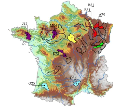
Fig. 2.Selected catchments are identified with the first three digits of each code used in Table 1. The other delimited basins are part of the study of results’ generalization shown in Brochero et al. (2011).

It is possible that the NS evaluated in the selected sets with BGS hides undesirable effects on the balance of the scores, for example to substantially improve one score with respect to the other score(s). To check this condition, a gain index for each score is also proposed:

GSC(%)= 100 ×

Scoreie −Scorese

|Scoreie| . (9)

A positive index indicates superior performance of the se-lected set. The absolute value in the denominator is needed to assess the performance of IGNS, which can have positive and negative values.

3 Experimental set-up

Figure 1 shows the selection procedure applied to the 800-member HEPS. The main elements of the methodology are described below.

3.1 Database: 800-member HEPS

Database details can be found in Vel´azquez et al. (2011). The study is conducted over 10 French catchments with a typical response time of 3 days. These catchments represent a large variety of hydro-climatic conditions (Fig. 2 and Table 1), and were evaluated over a period of 17 months (from March 2005 to July 2006).

(6)

Table 1. Main characteristics of the studied basins (mean annual values) based on a 36 year length of the series (1970–2006).

Catchment Area Altitude P ET Q

codes (km2) (m a.m.s.l.) (mm) (mm) (mm)

A7930610 9387 155 2.78 1.80 1.21

B2130010 2290 227 2.57 1.80 0.87

B3150020 3904 162 2.58 1.80 1.09

H3621010 3900 48 1.98 1.95 0.45

J8502310 2465 4 2.36 1.89 0.81

K7312610 1712 85 2.13 2.01 0.68

M0421510 1890 56 2.04 1.89 0.62

O3401010 2170 349 3.19 1.80 1.90

Q2593310 2500 17 2.52 2.24 0.75

U2542010 4970 201 3.63 1.75 1.88

P: precipitation, ET: potential evapotranspiration, Q: flow.

were used for the calibration and validation of the hydrolog-ical models. Observed data for the period 11 March 2005 to 31 July 2006 was used only for the evaluation of the forecasts. The forecast verification period is thus indepen-dent of the calibration/validation period. Rainfall data come from the meteorological analysis system SAFRAN of M´et´eo-France (see Quintana-Segu´ı et al., 2008 for details). They consist of rainfall accumulated at a daily time step and avail-able for the entire country of France at an 8_×8-km grid reso-lution. Daily streamflow data come from the French database Banque Hydro (http://www.hydro.eaufrance.fr/). The length of available observed streamflow time series varies accord-ing to the catchment, with, on average, 29 years of available daily data for the catchment dataset used here.

The 50 perturbed forecasts from ECMWF was provided at a 0.5◦×0.5◦lat/lon grid resolution. A detailed description of the ECWMF EPS model can be found in Molteni et al. (1996) or Buizza (2005). Forecasts are issued at 12:00 UTC and ex-tend over 240 h. Rainfall amounts were accumulated at 24 h time steps, starting at 0 h to match with observed daily data, which resulted in nine daily lead times. No bias removal or disaggregation was performed. For each catchment, areal mean rainfall forecasts were computed by averaging the rain-fall amounts of each grid above the catchment, weighted by the percentage of the catchment area inside the grid.

The sixteen hydrological models are lumped models and correspond to various conceptualizations of the rainfall-runoff transformation at the catchment scale. Some origi-nal model structures were modified. Thus, to avoid unfair comparisons of models, they will be referred to hereafter as HM## (Table 2). It is beyond the scope of this article to present these models. References with a detailed explana-tion of each model structure can be found in Vel´azquez et al. (2011).

On the other hand, analysis of the median coefficient of variation (MDCV), as a measure of the diversity of the HEPS, revealed the following characteristics:

Table 2.Hydrological models.

Hydrological Base model and Hydrological Base model and models parameters models parameters

HM01 CEQU 9 HM09 CREC 8

HM02 GR3J 3 HM10 GR4J 4

HM03 HBV0 9 HM11 SIMH 8

HM04 IHAC 6 HM12 MOHY 7

HM05 MORD 6 HM13 PDM0 8

HM06 SACR 13 HM14 HYM0 5

HM07 SMAR 9 HM15 TANK 10

HM08 TOPM 8 HM16 WAGE 8

– The variability is low at least for the first three days of predictions (MDCV<0.12), many models showing no variability (i.e. the same response for all members). As shown by Vel´azquez et al. (2011), part of this difficulty may be inherited from the meteorological ensembles, which are not reliable prior to about a 3-day lead time. More importantly, it is believed that not including un-certainties associated with the hydrological initial con-ditions at the onset of the forecasts takes its toll on re-liability, at least for the first few time steps of the hy-drological predictions, i.e. until the mean characteristic response time scale of the studied catchments (3 days) is reached.

– As for the incremental variability, it depends on the forecast horizon. MDCV for 4 to 9-day predictions reached between 0.2 and 0.6, respectively.

Consequently, the results presented in this paper are strictly based on the 9-day forecast horizon. This decision is justified on the variability within the ensemble forecasts as well as on the fact that the selection of hydrological members as a method of simplifying HEPS should be unique regard-less of the forecast horizon. The companion paper (Brochero et al., 2011) assesses the transferability of the 9-day mem-bers’ selection to other forecast horizons.

3.2 Resampling technique

In some algorithms, such as the BGS, the overfitting1is high-lighted as a structural problem. So, one method for improv-ing generalization which is called early stoppimprov-ing (Hudson and Demuth, 2011; Alpaydin, 2010), well-known in the neu-ral network community, is used in the methodology proposed here.

In this technique, the available data is divided into three subsets. The first subset is the training set, which is used in BGS for sequentially removing the members. The second subset is the validation set. The error on the validation set

1_{When the error on the training set is driven to small values, but}

(7)

is monitored during the training process. The validation er-ror normally decreases during the initial phase of training, as does the training set error. However, when the selection begins to overfit the data, the error on the validation set typ-ically begins to rise. When the validation error increases for a specified number of members, the training is stopped. The test set error is not used during training, but it is used to com-pare different models.

The need to define three subsets to run the BGS and the short length of the series impose the use of resampling tech-niques such ask-fold cross-validation, which maximizes the utilization of the available information.

Moreover, one notes the high degree of linear correlation exhibited in the first lags of the correlogram of the flow se-ries at hand (e.g. in the 80 % of the catchments evaluated, the correlation using a lag of three days was greater than 0.82). So, the choice of the training and validation data should be directed in order to temporarily avoid near data to form the two subsets. For example, suppose that the linear correlation betweenot andot+1is equal to 0.8 and that the selection of members has been trained inot and validated inot+1. The validation could consequently be highly contaminated by the effect of the correlation between data. Correlation contami-nation is avoided by forming training and validation subsets from groups of 10 consecutive data (blocks) rather than from individual data. It is important to note that contrarily to stan-dard hydrology applications, the order of the events is not important in the BGS process.

Here, the dataset is divided into 5 equal-sized parts in or-der to create 5 experiments. In each experiment, a part is kept out for testing, while the remaining four parts, a priori divided in blocks, are randomly combined to form training and validation subsets. The detailed process develops in two steps:

– Step 1: Data and test set configuration. The test set is set-up from simple cut-offs to “guarantee” statistical independence with the training-validation process. To build the test set, the series is subdivided into five folds, each of which corresponds to the test set of each ex-periment. For example, ifN denotes the length of the series, the test set of the first experiment corresponds to the first fold (i= 1 to ⌊N/5⌋), similarly the test set of the fifth experiment will be the last fold (i=⌈4N/5⌉

toN). Thus, strong linear correlation between training-validation and the test dataset is limited only to the val-ues situated near the cut-off line.

– Step 2: Blocks’ selection of the training and validation sets. The remaining 4 parts are grouped intokblocks of consecutive pairs of observations-ensemble forecast, then randomly choosing 75 % of the blocks for the train-ing set and the remaintrain-ing 25 % sets for the validation set.

3.3 Backward Greedy Selection (BGS)

In Machine Learning, the evaluation of multiple models for simulation or prediction of an event, and to further select those which together enhance or simplify a condition for ad-justment, is known as an overproduce and select. In a gen-eral context of selection, numerous methods have been devel-oped. There are greedy selection methods (Backward or For-ward Selection) but also methods such as integer program-ming and evolutionary algorithms.

Here, BGS and the idea of subdividing the data into three subsets to improve the generalization are applied. For its im-plementation it is necessary to define the error function “E” (that it is one of the given statistical scores shown in Sect. 2) and the minimum number of members. With regard to the minimum number of members, which was arbitrarily defined as 30 here, the choice is mainly due to the high availability of initial members (800), for example with 30 hydrological members a level of compression of information equivalent to 96.25 % is reached. It is certain that if the selection task had started with a pool of 50 members, then the minimum number of members could have been defined as 10, for ex-ample. Moreover, the minimum number of members is just a stopping criterion of selection with BGS because the num-ber of memnum-bers to define as optimal should focus on specific analysis in each basin.

The members’ elimination mechanism begins with all members (d) and removes them one by one, at each step re-moving the one that decreases the error the most (or increases it the least). The removal mechanism is as follows:

1. It begins with a subdivision of the dataset (χ) into train-ing (χt), validation (χv), and test set (χp).

2. The reference set Gd_{, containing all of the original}_d members, is presented.

Gd _{= {}y₁,y₂,y₃, ...,y_d_}

3. For iter =d₋1,d₋2, ..., nmin

The hydrological member “y_j” corresponds to the one that, when it is removed, has the greater impact on the training set errorE(i.e. minimise train error the most). It is important to note thatEmust be a scalar or single value.

y_j ₌ argmin E Giter+1

\y_i _|χt yi∈Giter+1

The reference set is then updated by removing they_j

member inG. Giter ₌Giter+1_\y_j

4. At this point, the errorEin the validation setχ_v, ex-cluding they_j member, is evaluated.

(8)

5. The subsetGnminof the selected members is achieved, then the whole selection process is analysed on the training and validation results.

Backward Greedy Selection is a local search procedure that does not guarantee finding the optimal subset. For ex-ample, y_x andy_p by themselves may not be pertinent but together they may decrease the error substantially. But, because the algorithm is greedy and removes hydrological members one by one, it may not be able to detect this. Here, the BGS is executed with a resampling technique explained in Sect. 3.2.

3.4 Combination of results

The variability of each experiment set-up in the cross-validation step increases the probability of reaching different hydrological member’ selections. So, it is necessary to de-termine an integration mechanism for a global solution for each catchment. Here, the importance of each hydrological membery_i within the ensemble is then assumed as being di-rectly proportional to the iteration number at which it was eliminated during the selection process in each experiment (iteryi

xp). The combined ranking is thus the mean rank of

elim-ination as defined in Eq. (10):

R y_i

= 1

5

5 X

xp=1

iteryi

xp. (10)

For example, if the rank of elimination of the hydrological memberyiis 50, 60, 200, 10, and 150 in the five experiments, then the mean rank of elimination is equal to 94. Finally, the final selection (s) of thenm2best members corresponds to the members which have the highest mean rank of elimination given by Eq. (11):

s =

Rp, yp nm_p₌₁, Ri ≥ Rj where 1 ≤ i ≤ j ≤ d. (11) It should be noted that another possibility to integrating the results could have been based on the frequency of se-lection of each hydrological member of the ensemble, and later to elect the members with the highest frequency, but as this integration leads to a low performance, these results are omitted from this paper.

3.5 Interpretability of hydrological members’ selection In the case of MEPS in which the members are not perfectly interchangeable (e.g. Meteorological Service of Canada – MSC, TIGGE database), the selection of hydrological mem-bers with BGS focuses directly on the combinations of hy-drological members that maintain or improve characteristics of the super ensemble of reference.

2_nm _{is not necessarily equal to}_nmin _because_nm_{reflects the}

analysis of the error on the validation set regarding the number of selected members.

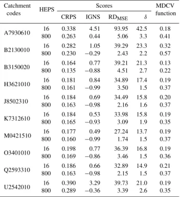
Table 3. Performance for the 16-member ensemble (16 hydrolog-ical models are driven by the deterministic forecast from ECMWF EPS) and the 800-member ensemble (16 hydrological models are driven by the 50 perturbed members forecast from ECMWF EPS) for a 9-day forecast time horizon. Hereafter, RD_MSE values are expressed on a 10−3basis.

Catchment codes HEPS

Scores MDCV

function CRPS IGNS RDMSE δ

A7930610 16 0.338 4.51 93.95 42.5 0.18 800 0.263 0.44 5.06 3.3 0.41

B2130010 16 0.282 1.05 39.29 23.3 0.32 800 0.230 −0.29 2.43 2.2 0.57

B3150020 16 0.164 0.77 39.21 21.3 0.13 800 0.135 −0.88 4.51 2.7 0.22

H3621010 16 0.181 0.84 34.89 17.4 0.19 800 0.161 −0.99 3.50 1.5 0.37

J8502310 ₈₀₀16 0.184_0.163 0.69 34.49 15.8 0.20 −0.98 2.16 1.6 0.37

K7312610 16 0.184 0.53 33.98 15.8 0.19 800 0.165 −0.93 3.09 1.9 0.35

M0421510 16 0.177 0.49 27.24 13.7 0.19 800 0.160 −0.99 1.74 1.5 0.37

O3401010 16 0.198 0.77 36.39 16.8 0.19 800 0.169 −0.86 3.46 1.5 0.36

Q2593310 16 0.186 0.66 32.89 14.9 0.21 800 0.163 −0.98 2.15 1.5 0.37

U2542010 ₈₀₀16 0.390_0.289 3.29 39.73 21.0 0.19 −0.36 3.39 2.6 0.35

But in the HEPS driven by a MEPS with interchangeable members (e.g. ECMWF EPS), the selection should be di-rected more clearly to a method of selection and weighting of hydrological models based on their participation in the fi-nal selected subset. Therefore, we can create a new simpli-fied high-performance HEPS using the same proportion of the hydrological members associated with a random choice of the meteorological members.

For example if the final selection shows that the simplified HEPS should consist of ten members for the hydrological model “A” and thirty members for the hydrological model “B”, then we should expect to achieve a high performance HEPS if we randomly pick ten meteorological members to evaluate the hydrological model “A” and thirty meteorologi-cal members, randomly chosen once again, to assess the hy-drological model “B”. Section 4.3 presents such an analysis.

4 Results and analysis

(9)

a desired behaviour. Note that theδratio and RDMSE, scores

on which rest the main advantages of the 800-member HEPS, are directly interpretable since the scale is independent of the measured variable.

With respect to the IGNS score, mean values are gener-ally negative, which shows that on average the system has an acceptable bias. Finally, in terms of CRPS, Vel´azquez et al. (2011) show in detail the efficiency of CRPS in this 800-member HEPS.

Note that results discussed in this paper correspond to a “pseudo test dataset” for comparing the performance be-tween different scores in the process of selecting hydrologi-cal members, since the data used to minimize all error func-tions are exactly the same.

It is a “pseudo test dataset” because there is a high proba-bility that the data used in testing (the complete series) have been used in the BGS training process, becoming the indi-cator of an optimistic estimator of the selection (Diaman-tidis et al., 2000); however, we do emphasize that the first part of this research focuses on an analysis of scores in the BGS process with the subsequent integration of results, and the second phase presented in a companion paper (Brochero et al., 2011) shows a rigorous test of generalization in time and space.

Validation results were omitted mainly because they have a trend similar to the training ones, except for some experi-ments where the random distribution of the training and val-idation sets was not statistically homogeneous.

In order to illustrate the interchangeability of the mem-bers of the ECMWF EPS and equiprobability of this system, Sect. 4.3 shows both the performance of the subset found with the BGS and the boxplot diagrams of 200 random ex-periments of 50 members, with and without the guidance of the BGS solution.

4.1 Selection performance

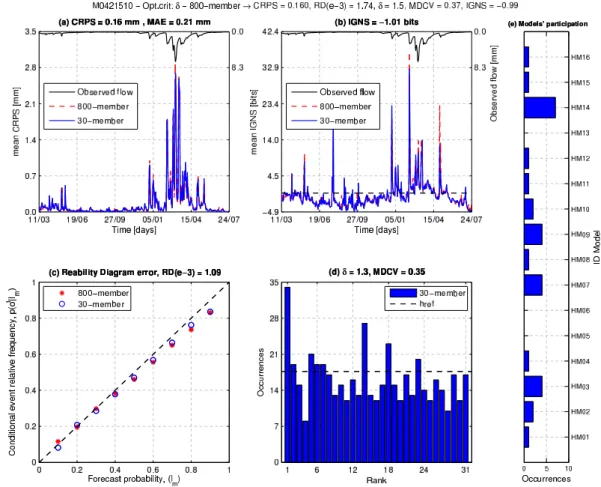
An example of the results obtained is shown in Fig. 3, which compares the 30-member and the 800-member results for the M0421510 catchment, after an optimization based on theδ criterion. In general the 30-member scores are better or as good as the reference set.

We stress the fact that the selection task focuses on the par-ticipation of the hydrological models. For instance, Fig. 3e shows that the selected hydrological members make use of 13 of the 16 available lumped models, however, the strong par-ticipation of the models 3, 7, 9, and 14 is displayed, which is an interesting combination of hydrological models, espe-cially taking into account the much poorer performance of the 16-member multi-model approach driven by the deter-ministic prediction (Table 3) and knowing that these hydro-logical models are not of equal quality with regards to MSE performance. This suggests that the selection favoured a di-versity of errors.

Specifically, Fig. 3a shows that the 30-member CRPS equals the reference value. Also, taking into account that the CRPS generalizes the Mean Absolute Error (MAE) for a point forecast (Gneiting and Raftery, 2007), it is impor-tant to stress that the CRPS values are always lower than the MAE values, when the deterministic counterpart was taken as the mean of each daily ensemble, in agreement with results obtained by other authors (Boucher et al., 2009; Vel´azquez et al., 2011). Another remarkable feature of CRPS is its di-rect relationship with the flow magnitude; the shapes of the CRPS and of the hydrograph are similar. A direct strategy of optimization could then focus on removing the hydrological members that have a large impact in the daily extreme CRPS values. Note also that the selection not only preserves the mean CRPS (0.16) but also the structure of the CRPS series. Figure 3b shows that the 30-member 4 % trimmed mean ignorance score (−1.01) has also improved over the initial value (−0.99). Regarding the time structure of the IGNS, it is observed that both the 30-member and 800-member values have many extreme values which suggest low assessments of the predictive distribution of the ensembles, i.e. a bias prob-lem in the forecasts (note that a value of 4.5 corresponds to an evaluation of thepdf near 0.0442).

With regard to the reliability diagram, Fig. 3c shows a con-siderable agreement improvement (1.09e-3) over the initial value (1.74e-3). This gain in reliability may be traced back to the optimization criterion used: theδ ratio, which is en-tirely based on the integration of the whole range in terms of corresponding verifications (observations). Similarly, Fig. 3d reveals that the rank histograms have a nearly uniform distri-bution, even if the first rank reflects a slight bias. Those im-perfections demonstrate the difficulty inherent in minimizing theδratio.

At the end of the selection process, the (MDCV) has slightly decreased, from 0.37 to 0.35. This confirms that op-timization with theδcriterion seeks diversity of the ensemble forecasts in the correct way, not necessarily maximizing the MDCV.

Figure 3e illustrates the occurrence of each lumped model from the 30-member ensemble. A wide selection of models alone could justify the multi-model approach advocated here. Results show that 13 models out of 16 were selected in this case, and that no models were selected more than 7 times.

(10)

Fig. 3.Comparison between the initial ensemble (800 members) and the ensemble selected (30 members) for the lead time 9 in the catchment M0421510. (a)Figure above: observed flow; figure below: CRPS, x-axis indicates day/month. Note the correspondence between higher observed flows and higher mean CRPS.(b)Figure above: observed flow; figure below: IGNS. Note that there is no full correspondence between the higher IGNS and higher observed flow, x-axis indicates day/month. (c)Reliability diagram error (RDMSEbased on vertical

distances between the points). (d)Rank histogram for the 30 selected hydrological members. The horizontal dashed line indicates the frequency (N/d+ 1) attained by a uniform distribution. (e)Occurrences of the employed models in the final solution of 30 hydrological members.

balance, i.e. evaluating that the normalized sum does not mask the detriment in a score(s) with gains made in other.

On the other hand, to reflect the BGS performance in the selection, Fig. 4 also presents the NS evaluation with 200 random selections of 30, 50, 100, 200, and 400 members in terms of gain index defined in Eq. (8). It is clear that BGS selection with positive gains are always obtained – improving the balance of the scores. Otherwise in random experiments the percentiles 10, 25, 50, 75, and 90 are shown generally in the range of a negative gain index (i.e. a detriment to the balance of the criteria). This tendency is obviously stronger in random selections of 100 or fewer hydrological members where the probability of taking the most representative hy-drological responses is lower. It is important to note how even in the random selection of 200 and 400 members (25 % and 50 % of the 800 hydrological members) the NS in 75 % of the evaluations shows a negative gain index.

To check each score individually, Table 4 shows the me-dian of 200 random selections for basin H36 optimized with the combined criterion. The random selections pick 50 hy-drological members to evaluate each score in a standardized fashion, that is, dividing the score obtained in the selection subset by the reference score of all 800 members of base (see each component in Eq. 7 without weight parameter).

Table 4 shows an analysis to evaluate the sensitivity of the scores with respect to the selection of hydrological members in the database under study. So, it is possible to point out the following:

– In the hydrological members’ selection, the greatest challenge is selecting a small set of members, for ex-ample 30 or 50.

(11)

Fig. 4. Evolution of the normalized sum (NS) in terms of gain index for the lead time 9, optimization with the combined criterion. Loga-rithmic scale on the x-axis. The normalized sum equal to 5 represents the performance of the initial 800-member ensemble. The thin red line represents the normalized sum under different numbers of members found with BGS. Symbols for the 200 random selection experi-ments: the blue vertical line identifies the interquartile range, white circles represent the median and yellow diamonds corresponding to the percentiles 10 and 90.

Table 4. Median of 200 random selections in catchment H36 for the lead time 9. The scores are presented in a standardized fashion and oriented at the minimization coinciding with the formulation of each component of the combined criterion (Eq. 7).

Members CRPS RDMSE δ MDCV IGNS NS

30 1.01 1.50 1.80 1.05 1.11 6.47 50 1.01 1.25 1.53 1.03 1.06 5.88 100 1.00 1.09 1.28 1.02 1.02 5.41 200 1.00 1.02 1.11 1.01 1.01 5.15 400 1.00 0.98 1.03 1.00 1.00 5.01

– The hydrological members’ selection presents its great-est challenges in maintaining or improving reliability and the consistency of the ensemble represented by the δ ratio, as shown in Table 3. Therefore, to define the combined criterion, such as an error term in BGS, the reliability term (RDMSE) has more weight to guide the

optimization in this way. At this point it should be noted that consistency has a direct relationship with reliabil-ity, although ensemble consistency does not necessar-ily imply that probability forecasts constructed from the ensemble are reliable in the sense of conditional out-come relative frequencies being equal to the forecast

Table 5.Results of BGS in catchment H36 for the lead time 9 with the combined criterion as error function. The scores are presented in a standardized fashion and oriented at the minimization coinciding with the formulation of the Eq. 7.

Members CRPS RDMSE δ MDCV IGNS NS

30 1.00 1.00 0.96 1.00 1.00 4.96 50 1.00 0.92 0.99 1.00 1.00 4.91 100 1.00 0.80 1.01 1.00 1.00 4.81 200 1.00 0.58 0.97 0.99 1.00 4.54 400 0.99 0.45 0.88 0.98 1.00 4.30

probabilities yielding a 45◦calibration function on a re-liability diagram, unless either the ensemble size is rel-atively large or the forecasts are reasonably skillful, or both (Wilks, 2011).

(12)

4.2 Scores interaction in the selection

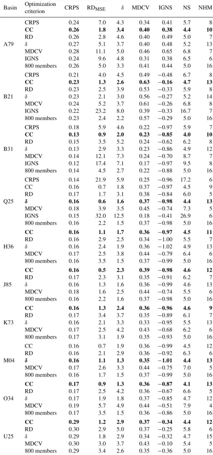
Table 6 summarizes results for more catchments and opti-mization criteria. The 30-member comparison is based on a normalized sum (Sect. 2.7). In this way, a value of NS lower than 5 indicates an overall improved performance. Per-formance for all criteria are also given in Table 6 for com-pleteness, and the best optimization criterion for each catch-ment is identified in bold letters.

Overall, the combined criterion (CC) offers an effective and direct rule, finding balance between features offered by each of the criteria. However, it is important to point out the two cases for which theδcriterion provides a slightly better optimum. This reflects the limitations of the BGS technique or the effects of the combination of results, because if the objective function (CC) is equal to the criterion used to com-pare results obtained with different objectives, the CC should obviously always find the best solution within the vision of a global optimization tool.

Theδ ratio criterion, based on a rank histogram which is the most common approach for evaluating whether a collec-tion of ensemble forecasts for a scalar predictand satisfies the consistency condition (Wilks, 2005), comes to a close sec-ond. It led to the best performance for two catchments and to the second best performance for five other catchments. This is particularly interesting considering the simplicity of this approach with respect to the combined approach. In addition, theδcriterion favoured the highest average participation of hydrological models.

The CRPS and IGNS led to a poorer selection, to the point that they were not considered further after experimenting with the first four catchments allowing an economy in com-putational time. The CRPS showed low variability, so it is not very sensitive to changes in the selection of hydrologi-cal members, as was shown in Tables 4 and 5. The IGNS demonstrated a negative relationship with reliability, leading to poor performance in terms of the reliability diagram (RD) andδratio. They are also correlated, optimizing one criterion often favouring the improvement of the other one.

Specifically the behaviour of the optimization of each score could also be described from the following relation-ships observed in Table 6:

– Optimization based on CRPS is detrimental to the reli-ability. For example, it had the effect of increasing RD by a factor of 10, for catchment Q25. The CRPS also decreases diversity of the members (MDCV), except for catchment B31 where it remained stable.

– The combined criterion (CC) leads to stable CRPS val-ues. The most remarkable gains come in terms of RD, as provided in the weights definition of the Eq. (7). With reference toδ ratio, evaluations reveal the difficulty in maintaining the stability of this criterion, but the dif-ferences between the selection and the reference set are not pronounced. As for the MDCV, the diversity is in

most cases maintained or improved. The IGNS perfor-mance is often slightly decreased. In conclusion, the CC promotes overall good performance, increasing the reliability of the system (decrease of the RDMSEscore)

and ensuring the stability in the other scores.

– Selection based on the RD score is detrimental to the CRPS. As for reliability, there are some cases for which the error increases. This condition is surprising given that the combined criterion always achieved reductions of this error, but it could not last under the assumption of a greater weight of this score in the combination be-cause the relationship is constant, which highlights the interaction between the scores as a mechanism implicit in the reduction of error reliability (RDMSE). Theδ

ra-tio is never improved, while diversity (MDCV) is lost except in three cases (B31, Q25, and U25) where inter-estingly the MDCV increased (theoretically consistent effect). Finally, the IGNS shows a negative trend to the minimization of the RD.

– By definition, theδ ratio focuses on the reliability and the consistency of the ensemble. In fact, it leads to bet-ter reliability performance in bet-terms of RD, than when the selection is optimized with RD itself. Theδ ratio also preserves the resolution of the forecast, as shown by the CRPS and IGNS results. All of this is accompa-nied by a slight loss in performance in terms ofδratio, which can be explained by the direct relationship of this score with the number of members. However, this de-pendency rather than becoming an obstacle in the selec-tion stands as a logical consequence of the system, since statistically a better performance is expected from a sys-tem that combines a larger number of members (Alpay-din, 2010). Finally, with respect to MDCV, it is shown once again that diversity, hypothetically represented by MDCV, fluctuates between values that indicate the ex-tent to which such diversity needs to be maintained in the ensemble.

– When the selection process focuses on the maximiza-tion of MDCV, the relamaximiza-tionship with CRPS, the IGNS andδratio is always negative. However, there are four cases in which the reliability is improved by increasing the diversity index, from which it follows that while re-liability improves the resolution drops.

(13)

Table 6.Selection of 30 hydrological members based on different scores in all the basins or the lead time 9. NHM indicates the number of hydrological models participating in the solution.

Basin Optimization

criterion CRPS RDMSE δ MDCV IGNS NS NHM

CRPS 0.24 7.0 4.3 0.34 0.41 5.7 8

CC 0.26 1.8 3.4 0.40 0.38 4.4 10

RD 0.26 2.8 4.6 0.40 0.49 5.0 7 A79 δ 0.27 5.1 3.7 0.40 0.48 5.2 13 MDCV 0.28 11.1 5.0 0.46 0.65 6.8 7 IGNS 0.24 9.6 4.8 0.31 0.38 6.5 6 800 members 0.26 5.0 3.3 0.41 0.44 5.0 16 CRPS 0.21 4.0 4.5 0.49 −0.48 6.7 8

CC 0.23 1.3 2.6 0.63 −0.16 4.7 13

RD 0.23 2.5 3.9 0.53 −0.33 5.9 8 B21 δ 0.23 2.1 3.0 0.56 −0.27 5.2 14 MDCV 0.24 5.2 3.7 0.61 −0.26 6.8 8 IGNS 0.22 23.2 8.0 0.39 −0.33 16.7 7 800 members 0.23 2.4 2.2 0.57 −0.29 5.0 16

CRPS 0.18 5.9 4.6 0.22 −0.97 5.9 7

CC 0.13 0.9 2.0 0.23 ₋0.85 4.0 10

RD 0.15 3.5 5.2 0.24 −0.62 6.2 8 B31 δ 0.13 2.9 3.3 0.23 −0.86 4.9 12 MDCV 0.14 12.1 7.3 0.24 −0.70 8.7 7 IGNS 0.12 17.4 7.1 0.17 −0.97 9.5 8 800 members 0.14 4.5 2.7 0.22 −0.88 5.0 16 CRPS 0.14 21.9 5.9 0.25 −0.96 17.2 6 CC 0.16 0.7 1.8 0.37 −0.97 4.5 9 RD 0.17 1.7 3.1 0.38 −0.84 6.0 5 Q25 δ 0.16 0.6 1.6 0.37 ₋0.98 4.4 13 MDCV 0.18 3.9 3.5 0.45 −0.74 7.3 5 IGNS 0.15 32.0 12.5 0.18 −0.41 26.9 6 800 members 0.16 2.2 1.5 0.37 −0.98 5.0 16

CC 0.16 1.1 1.7 0.36 ₋0.97 4.5 11

RD 0.16 2.9 2.5 0.34 −1.00 5.5 7 H36 δ 0.16 2.4 1.9 0.36 −1.02 4.9 13 MDCV 0.17 2.5 3.8 0.44 −0.79 6.4 6 800 members 0.16 3.5 1.5 0.37 −0.99 5.0 16

CC 0.16 0.5 2.3 0.39 −0.98 4.6 12

RD 0.17 2.3 3.1 0.35 −0.91 6.2 7 J85 δ 0.16 1.3 1.6 0.36 −0.99 4.6 13 MDCV 0.18 1.6 2.5 0.44 −0.74 5.5 6 800 members 0.16 2.2 1.6 0.37 −0.98 5.0 16

CC 0.16 1.3 2.4 0.36 −0.96 4.6 9

RD 0.17 3.4 3.7 0.35 −0.89 6.1 7 K73 δ 0.16 2.1 3.3 0.33 −0.95 5.5 13 MDCV 0.17 2.5 4.2 0.43 −0.68 6.2 6 800 members 0.17 3.1 1.9 0.35 −0.93 5.0 16

CC 0.16 0.7 1.9 0.36 −0.99 4.5 12 RD 0.16 2.1 2.9 0.36 −0.92 6.3 6 M04 δ 0.16 1.1 1.3 0.35 ₋1.01 4.4 13 MDCV 0.17 2.6 3.3 0.44 −0.75 7.0 5 800 members 0.16 1.7 1.5 0.37 −0.99 5.0 16

CC 0.17 0.9 1.3 0.36 −0.87 4.1 13

RD 0.17 2.5 4.2 0.36 −0.67 6.6 5 O34 δ 0.17 1.9 1.8 0.37 −0.85 4.7 12 MDCV 0.19 5.7 4.9 0.44 −0.51 7.9 4 800 members 0.17 3.5 1.5 0.36 −0.86 5.0 16

CC 0.29 1.2 2.9 0.37 ₋0.34 4.4 12

(14)

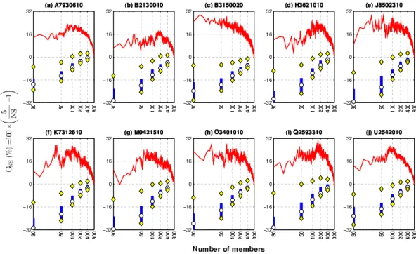
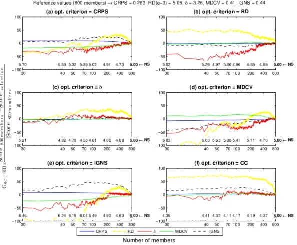
Fig. 5.Evolution of the gain index for each score under different optimization schemes in the basin A79 for the lead time 9. A logarithmic scale is used on the x-axis. The chosen optimization criterion in the selection is shown at the top of each subfigure. The lower part of each subfigure indicates the values of the normalized sum (NS) for the number of hydrological members shown on the x-axis.

be understood from a theoretical point of view. Theδ ratio improves reliability while maintaining resolution. The com-bined approach stands out as the most balanced criterion.

The above analysis focused exclusively on 30-member se-lections. However, a global vision requires the analysis of the evolution of the scores as the number of hydrological mem-bers is reduced. Such an analysis is specific to each catch-ment, so as an example, Fig. 5 shows evolution diagrams of the various scores as a function of the number of members, for the catchment A79.

In order to assess the joint evolution of all scores the gain index defined by Eq. (9) was used. Figure 5a and 5e clearly show that an optimization based on resolution of the sys-tem (CRPS or IGNS) is detrimental to the reliability. Fig-ure 5 also highlights the correspondence of CRPS and IGNS throughout the selection process, when the optimization is focused on one or the other.

RD optimization (Fig. 5b) is surprisingly unfavourable to theδratio (negative gain index), which is related to the indif-ference of the RD with respect to the location of the observa-tion within the ensemble, while this locaobserva-tion analysis creates a solid indicator of the system consistency. Likewise, it is

remarkable that the normalized sum for RD is equal to 4.96 when the number of hydrological members is equal to 100. This is strictly because loss in consistency (negative gain in-dex in theδratio of 40 %) and resolution (IGNS equivalent to losses of 10 %) is balanced by a positive gain of about 50 % in RD.

Theδ ratio (Fig. 5c) displays a gradual overall improve-ment of individual scores in a selection of about 70 hydro-logical members, when the various scores show a tendency to decrease in performance. At this point it is important to note that the normalized sum (NS) reached 4.53.

Figure 5d shows that criteria focusing on the resolution and the consistency have a negative relationship with the maximization of the diversity (MDCV), overall gains are achieved only when the number of hydrological members is greater than 400.

(15)

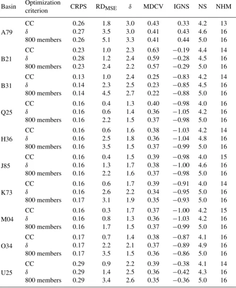
Table 7. Selection of 100 hydrological members based on the combined (CC) andδcriteria. NHM indicates the number of hydrological models participating in the solution.

Basin Optimization

criterion CRPS RDMSE δ MDCV IGNS NS NHM

A79

CC 0.26 1.8 3.0 0.43 0.33 4.2 13

δ 0.27 3.5 3.0 0.41 0.43 4.6 16

800 members 0.26 5.1 3.3 0.41 0.44 5.0 16

B21

CC 0.23 1.0 2.3 0.63 ₋0.19 4.4 14

δ 0.28 1.2 2.4 0.59 ₋0.28 4.5 16

800 members 0.23 2.4 2.2 0.57 ₋0.29 5.0 16

B31

CC 0.13 1.0 2.4 0.25 ₋0.83 4.2 14

δ 0.14 2.3 2.5 0.23 ₋0.85 4.5 16

800 members 0.14 4.5 2.7 0.22 ₋0.88 5.0 16

Q25

CC 0.16 0.4 1.3 0.40 ₋0.98 4.0 16

δ 0.16 0.6 1.4 0.36 ₋1.05 4.2 16

800 members 0.16 2.2 1.5 0.37 ₋0.98 5.0 16

H36

CC 0.16 0.6 1.6 0.38 ₋1.03 4.2 14

δ 0.16 2.5 1.8 0.36 ₋1.04 4.8 16

800 members 0.16 3.5 1.5 0.37 ₋0.99 5.0 16

J85

CC 0.16 0.4 1.5 0.39 ₋0.98 4.0 15

δ 0.16 1.3 1.7 0.38 ₋1.00 4.6 16

800 members 0.16 2.2 1.6 0.37 ₋0.98 5.0 16

K73

CC 0.16 0.6 1.7 0.39 ₋0.91 4.0 14

δ 0.16 2.6 2.2 0.34 ₋0.95 5.0 16

800 members 0.17 3.1 1.9 0.35 ₋0.93 5.0 16

M04

CC 0.16 0.3 1.7 0.37 ₋1.00 4.2 15

δ 0.16 0.8 1.3 0.36 ₋1.03 4.2 16

800 members 0.16 1.7 1.5 0.37 ₋0.99 5.0 16

O34

CC 0.17 0.7 1.4 0.38 ₋0.87 4.1 16

δ 0.17 2.2 2.1 0.37 ₋0.89 4.9 16

800 members 0.17 3.5 1.5 0.36 ₋0.86 5.0 16

U25

CC 0.29 0.9 2.2 0.39 ₋0.38 4.1 14

δ 0.29 1.4 2.5 0.36 ₋0.42 4.3 16

800 members 0.29 3.4 2.6 0.35 ₋0.36 5.0 16

Table 7 groups the 100-member scores following opti-mization with the combined score and the δ ratio, the two best ones. These values confirm the superiority of the com-bined score, leading to the smallest NS for all catchments, mainly because of the great influence on minimizing relia-bility. This also maximizes MDCV to such an extent that it allows a proper balance between reliability, resolution, and consistency. It is also remarkable that for 8 catchments out of 10, the δ ratio is minimized even more than when the optimization is focused on theδ ratio itself. Optimization based on theδratio also improved scores over the initial 800-member values (NS<5) for 9 catchments out of 10. This single criterion is thus also very appealing, especially be-cause it makes use of all 16 models in its selection.

Additionally, the δ ratio can be highlighted as a simple optimization criterion, which for 100 % of the catchments,

makes use of the participation of all hydrological models in the formation of the solution, which is not the case for the optimization with the CC.

4.3 Interchangeability of MEPS members as input of hydrological models

(16)

of results under different random selections but without con-sidering the participation of hydrological models found with BGS.

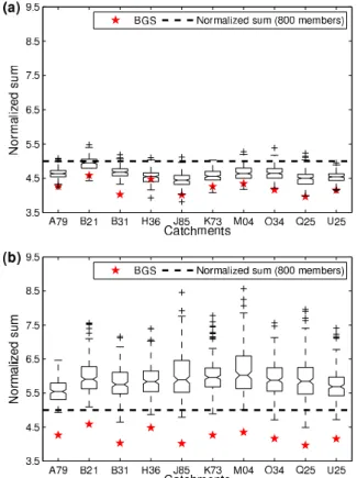
Figure 6 highlights three main aspects: high-performance solutions based on the proportion given by the BGS, low vari-ability, and high performance of the BGS solutions.

The performance of selections based on the proportion of members found in the BGS solution is evident in Fig. 6a. So, it is demonstrated that the proportion of members for a hy-drological model is generally a sufficient criterion to reduce the number of members while improving the balance of the scores represented by the normalized sum. For comparison, Fig. 6b illustrates the system response to random selections without any a priori guidance, showing that in all cases the normalized sum is greater than 5 and have recurring extremes greater than 7.

Regarding the variability of the normalized sum evaluated in random selections guided by the BGS solution, it can be seen that the interquartile range (Q3−Q1) is at worst equal

to 0.3 (catchment H36), which is a much lower value than for the purely random selection, as shown in Fig. 6b where the latter interquartile range is equal to 0.6.

The generalization of the BGS method is discussed in de-tail in the companion paper, where the temporal and spatial generalization is evaluated for a nearby catchment. However, Fig. 6a shows that the catchments H36 and J85 obtained com-binations with a normalized sum lower than those obtained with the BGS method (see only cross points at the bottom in Fig. 6a), which can be associated with the integration of experiments carried out in a subdivision database for each catchment or the BGS algorithm structure – it is known that the classical BGS algorithm is unable to detect the collective influence of the variables.

5 Conclusions

Previous results on the number of hydrological members and the HEPS conformation (Vel´azquez et al., 2011) have shown, based on the database of the present paper, that the ensem-ble predictions produced by a combination of several hydro-logical model structures and meteorohydro-logical ensembles (800-member set) have higher skill and reliability than ensemble predictions given either by a single hydrological model fed by weather ensemble predictions (50-member set) or by sev-eral hydrological models driven by a deterministic meteoro-logical forecast (16-member set). So, our goal was focused on at least replicating the good quality of the 800-member set with fewer hydrological members.

Hydrological member selection is justified by the com-putational cost to issue a hydrological forecast based on the combination of meteorological models and hydrological models. In this line, the selection of hydrological members without sacrificing the quality of a forecast stands out as an operational option.

Fig. 6. Backward Greedy Selection (BGS) and Box-plots in 200 random experiments of 50 hydrological members for the lead time 9. On each box, the central mark is the median, the edges of the box are the 25th (Q₁) and 75th percentiles (Q₃), the whiskers or limits to consider the outliers extend fromQ1−1.5×(Q3−Q1)

toQ3+ 1.5×(Q3−Q1) points (but not necessarily correspond to

observed data), and the outliers are plotted individually as cross points.(a)Random selection oriented with the frequency observed in the BGS to check the interchangeability in the 800 member-set,

(b)Random selection without any guidance to check the BGS per-formance.

Results presented here support the idea that selecting HEPS members is viable. It is in general even possible to expect a better balance of scores in the subset of selected hy-drological members than in the original much larger ensem-ble, based on standard scores such as the CRPS, the IGNS, the reliability diagram, and theδratio. The diversity, sought in the multi-model approach with MEPS, may also be main-tained in the final selection.

(17)

with a number of members fluctuating between 30 and 100, maximizing the qualities of the system: reliability, consis-tency, resolution, and diversity. So in the worst case this corresponds to a 87.5 % (700 members/800 members) com-pression level. The ultimate level of comcom-pression is in fact a compromise between the gain index and the complexity of the system. The ultimate decision should be established ac-cording to the requirements and the operational capacity of the hydrological probabilistic forecast system.

The evaluation of five individual scores as criteria for op-timizing the selection process revealed the complexity of the relationship between them. In many situations, improving one score is achieved at the expense of another score. There-fore, the design of a combined criterion (CC) led to an impor-tant methodological improvement that integrates many char-acteristics of each score. Theδ ratio is the best single op-timization criterion, not very distant to the achievements of the combined criterion (CC).

The CRPS is often the primary score used for evaluating HEPS performances. However, results here indicate that it is not a good choice for hydrological members’ selection in this case of study. In fact, it was often possible to preserve or minimize the CRPS using other objective criteria. Like-wise, the centralization of the selection process in the IGNS heavily penalized the reliability and the consistency of the system. With respect to the MDCV, the uncontrolled maxi-mization of this parameter, which describes diversity, leads to a deterioration of the other sought qualities of the system. There exists a threshold beyond which the system abruptly loses reliability, resolution, and consistency. On the other hand, experiments showed that both theδ ratio and the CC improve the balance of the scores.

The proposed methodology is part of the so-called data-driven models, so the design is independent of the database, in this case the evolution of MEPS or hydrological models. Precisely this point stands out as one of the advantages of the proposed methodology, since the selection of hydrological members could be implemented in any desired combination between any MEPS (e.g. ECMWF EPS, MSC, US National Centers for Environmental Prediction – NCEP) and hydro-logical models.

The cross-validation, a vital part of the proposed method-ology, systematically deals with the issue of the short length of the series. However, it is widely applicable to any length of condition series.

Finally, the encouraging results of this study will lead to an interest in testing other global search (non-greedy) tools such as evolutionary algorithms.

Appendix A Notations

t Time-step

N Number of pairs

observations-forecasts

d Total number of hydrological

mem-bers in the forecast ensembles M Total number ofmintervals to

anal-yse the reliability diagram

c Identification of the rank or class to analyse the uniformity in the rank histogram

ot Observed flow at the timet

yt Ensemble flow forecast at the timet y_it i-th flow forecast member inyt

Y Ensemble flow forecast from t= 1

toN