SOIL FERTILITY EVALUATION FOR FERTILISER RECOMMENDATION USING
HYPERION DATA
Ranendu Ghosh a *, N. Padmanabhanb, K.C. Patel c,
a Professor, DA-IICT, Gujarat 382 007, India –[email protected]
b Professor, Ahmedabad University, Ahmedabad, Gujarat, India - [email protected]
c Associate Professor, Anand Agriculture University, Anand 388110, Gujarat , India –[email protected]
KEY WORDS: Soil fertility, Soil testing, Hyperion, Hyperspectral, Spectral Feature Fitting (SFF), Pixel Purity Index (PPI),
Correlogram.
ABSTRACT:
Soil fertility characterised by nitrogen, phosphorus, potassium, calcium, magnesium and sulphur is traditionally measured from soil samples collected from the field. The process is very cumbersome and time intensive. Hyperspectral data available from Hyperion payload of EO 1 was used for facilitating preparation of soil fertility map of Udaipur district of Rajasthan state, India. Hyperion data was pre-processed for band and area sub setting, atmospheric correction and reflectance data preparation. Spectral analysis in the form of SFF and PPI were carried out for selecting the ground truth sites for soil sample collection. Soil samples collected from forty one sites were analysed for analysis of nutrient composition. Generation of correlogram followed by multiple regressions was done for identifying the most important bands and spectral parameters that can be used for nutrient map generation.
1. INTRODUCTION
Accurate soil information is crucial for management decisions like crop specific fertilizer recommendation. Traditionally, soil variability has been studied and summarized in soil surveys. These studies delineate soil boundaries, by partitioning continuous soil variability into discrete soil units described by taxonomic variability.
With the availability of imaging spectroscopy data, the possibilities for soil science applications have increased to a great extent. This is due to the inclusion of shortwave infrared region of the reflected spectrum combined with high spectral resolution and contiguous placement of bands, while keeping an acceptable spatial resolution.
Soil minerals, organic matter, and moisture are the major components of soils, with distinct spectral features in the visible and near-infrared regions (Stoner & Baumgardner, 1981, Clark, 1981). Soils generally have similar reflectance spectra in the 1100 to 2500 nm, including three distinct absorption peaks around 1400, 1900 and 2200 nm and a few small absorption peaks between 2200 and 2500 nm. Other than strong response of soil moisture at 1400 and 1900 nm, the absorption peaks for soils in the infra-red region are difficult to assign to specific chemical components. Near-infrared Reflectance Spectroscopy (NIRS) has been used successfully to predict organic carbon (OC) and total N content of the soils (Chang & Laird, 2002). However levels of organic carbon and total N in soils are strongly correlated. Therefore, it is not clear if predictions of total N in soils by NIRS are based on spectral features of N containing organic functional groups or are caused by autocorrelation.
2. OBJECTIVES
Pre-processing and analysis of Hyperion data
using standard algorithm available in
commercial software.
Determination of soil fertility status of the soil
sampling sites from laboratory chemical
analysis.
Establish the statistical relationship between
fertility status with respect to major nutrients e.g.
organic carbon, nitrogen, phosphorus,
potassium, calcium, magnesium and sulphur with spectral parameters.
Prepare soil fertility map with respect to the
seven nutrients of the study area using the above relationship.
3. STUDY AREA
The study area corresponds to Udaipur district in Rajasthan
bound by the following lat – long
Top Left: 24o54'47’'N, 73o44'13’'E
Top Right: 24o53'53'’N, 73o48'39’'E
Bottom Left: 24o07'49’'N, 73o32'52’'E
Bottom Right: 24o06'55’'N,
73o37'16’'E
4. MATERIALS
4.1 Satellite data
One date Hyperion (date of acquisition 19 January 2004) from EO-1 and IRS L3 data (date of acquisition January 2004) were used for this study.
The Hyperion instrument provides radio metrically calibrated spectral data. Hyperion is a push broom, imaging spectrometer. Each ground image contains data for a 7.65 km wide (cross-track) by 185 km long (along-(cross-track) region. Each pixel covers an area of 30 m x 30 m on the ground, and a complete spectrum
covering 400 – 2500 nm is collected for each pixel.
IRS L3 geo-referenced FCC (23.5 meter spatial resolution) was used for geo-rectification of processed Hyperion data so that GIS and satellite data can be viewed from the same spatial framework for further analysis.
4.2 Archived GIS data
Archived GIS database including lithology, soils and administrative boundaries were used as reference for the study.
5. METHODS
5.1 Pre-processing of Hyperion data: Hyperion Level 1
radiometric product has a total of 242 bands but only 198 bands are calibrated. Because of an overlap between the VNIR and SWIR focal planes, there are only 196 unique channels. The bands that are not calibrated are set to zero. A typical Hyperion image has the dimensions of 256 (number of pixels) x 6925 (number of frames) x 242 (number of channels). Spectral
resolution of all the bands is in the range of 10 – 11nm.
5.1.1 Spatial and spectral sub setting: Top portion of the
image (North) was seen to be covered with clouds which could not be used for analysis. Therefore the original image was sub-setted to 3026 lines that were used for analysis purpose.
As explained above from original 242 channels, only 196 channels were calibrated. Twenty one out of 196 channels were deleted since these are falling within water absorption band in
the range 1356 – 1416 and 1810 – 1941 nm. The radiance
values were recorded as zero in these ranges and so were deleted from the list of 196 channels. The number of channels finally used for analysis was 175.
5.1.2 Atmospheric correction and conversion to reflectance image: ENVI’s Fast Line-of-sight Atmospheric Analysis of Spectral Hypercubes (FLAASH) module is a first-principles atmospheric correction modelling tool for retrieving spectral reflectance from hyper spectral radiance images (FLASSH, 2006).
The parameters for ENVI FLAASH include selecting an input radiance image, setting output file defaults, entering information about the sensor and scene, selecting an atmosphere and aerosol model, and setting options for the atmosphere correction model.
5.1.3 Geo-referencing of Hyperion image: Radiometrically
corrected product was corrected to geo reference the reflectance image and transform in the same spatial reference system with
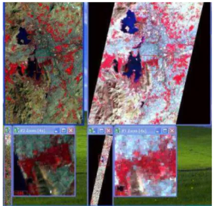
the collateral database. The corrected image after pre-processing is shown in Fig. 1.
Fig 1 Original radiance and pre-processed Hyperion reflectance image
5.2 Spectral analysis: Spectral analysis of Hyperion
reflectance image was primarily focused to select the optimum number and location of ground truth sites based on some objective criteria.
5.2.1 Spectral Feature Fitting (SFF) matches the image
pixel reflectance spectrum to reference spectrum from either a spectral library or field spectrum after continuum removal is applied to both image and reference spectrum (Clark et. Al 1991). The continuum is removed using (Clarke & Rouse, 1984).
ec () = e () / ce () (1)
fc () = f () / cf ()
where ec () is the continuum removed reference spectrum and
fc () is the continuum removed image reflectance spectrum,
respectively. The resulting normalized spectra reflect levels equal to 1.0 if the continuum and the spectrum match and less than 1.0 in the case of absorption.
Similarly the absorption feature depth is defined as, for each
spectrum
D[ec ()] = 1 - ec () = 1 - e () / ce () (2)
D[fc ()] = 1 - fc () = 1 - f () / cf ()
Scaling is usually necessary for reference spectra because absorption features in library data typically have greater depth than image reference spectra. The scale image, produced for each reference mineral, is the image of scaling factors used to fit the unknown image spectra to the reference spectra. The
result is a grayscale image, whose DN value corresponds to S
(x). The total root mean square (RMS) errors, is defined as E
(x). The fit image equals
F (x) = S (x) / E (x) (3)
providing a measure of how well image pixel reflectance
spectra match reference spectra. A large value F (x)
corresponds to a good match between the image spectrum and the reference spectrum (Debba et. al. 2005)
A sample fit image is shown in Fig 2
Fig 2 SFF fit image of Illite clay mineral.
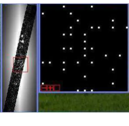
5.2.2 Pixel Purity Index (PPI)(ENVI User’s Guide) finds the
most spectrally pure (extreme) pixels in multispectral and hyperspectral images. These typically correspond to mixing end members. The PPI is computed by repeatedly projecting n-D scatter plots on a random unit vector. ENVI records the extreme pixels in each projection (those pixels that fall onto the ends of the unit vector) and it notes the total number of times each pixel is marked as extreme. A Pixel Purity Image is created where each pixel value corresponds to the number of times that pixel was recorded as extreme. The PPI function can create a new output band or continue its iterations and add the results to an existing output band. The PPI is typically run on a Minimum Noise Fraction (MNF) transform result; excluding the noise bands. Fig 3 depicts the PPI image generated from the processed Hyperion data which was finally used for selecting the soil sampling sites.
Fig 3 PPI image of the area.
All the images after SFF and PPI processing were converted into vector (point) to compare with the GIS database like lithology, soil and select sites for soil sampling.
5.3 Soil chemical analysis:
5.3.1 Soil Organic Carbon (Jackson, 1973) Organic carbon
was estimated from potassium chromate and sulphuric acid solution and keeping the solution for overnight. The green chromus color of the clear liquid is measured in spectrophotometer using 645 nm (red filter) and compared with the standard curve for OC estimation.
5.3.2 Available Nitrogen (Jackson, 1973) Available nitrogen in
the soil is measured by distillation method using 0.32% KMnO4
and 2.5% NaOH solution. Distillation process is followed by titration with std. 0.1 N H2SO4.
5.3.3 Available Phosphorus (Olsen et. al. 1954) Available
phosphorus in the soil is estimated by spectrophotometric
method. Soil phosphorus is extracted using 0.5M NaHCO3 (pH
8.5) solution and activated charcoal followed by addition of ammonium molybdate solution. The extract is measured in spectrophotometer with the help of 660 nm wavelength (red filter) and compared with standard curve for phosphorus concentration.
5.3.4 Available Potassium (Jackson, 1973) Available
potassium in the soil is measured through flame photometric method. Potassium from soil is extracted using 1N ammonium acetate (pH 7.0) solution followed by filtration. The filtrate is taken for measurement.
5.3.5 Available Potassium (Williams, and Steinbergs 1959)
Available phosphorus is also measured through
spectrophotometric method at 430 nm wavelength. Sulphur in the soil is extracted using 0.15 % CaCl2 solution followed by
adding BaCl2 powder to the extract. The sample curve is
compared with standard for calculating sulphur concentration.
5.3.6 Exchangeable Calcium and Magnesium (Jackson, 1973)
Available calcium and magnesium in soil are normally designated as those which are found in the exchangeable form. Total exchangeable Ca + Mg and Ca alone in soil are measured using EDTA titration method. Magnesium is then calculated indirectly after subtracting Ca content from total Ca + Mg content.
All the seven nutrients, except exchangeable Ca and Mg, were categorised into three groups low, medium and high. These tables are presented in Appendix.
5.4 Statistical analysis: Statistical analysis was primarily
aimed at optimizing number of bands and the spectral parameter from soil nutrient and reflectance data of 41 soil sampling sites. The spectral parameters considered for the analysis are as follows
Reflectance = R
First derivative of R (R’) = (R - R-1 ) / ∆
Absorptance (A) = log10 (1/R)
First derivative of A (A’) = (A - A-1 ) / ∆
where ∆ is the spectral interval between two subsequent
spectral bands.
As it is known that spectral bands are highly correlated which creates lot of redundancy and computer overhead in data processing. Also for certain nutrients a particular wavelength region or bands may be more significant than others. Therefore for selecting the bands significant for a particular soil nutrient, spectral parameters were linearly correlated against the analyzed value of the given soil nutrient. A correlogram spectrum for each nutrient, showing the correlation coefficient versus the wavelength, was performed for each spectral parameter and soil nutrient separately. The spectral bands at which the correlation coefficient exceeds a threshold value were selected for multiple regressions (Ben-Dor et. al., 2002).
Selection of spectral bands was followed by selection of one spectral parameter, out of four mentioned earlier, to establish the multiple regression coefficients to be used for generating the fertility image. Forward regression model assumed to generate the coefficients are as follows
Cp = B0 + B1 R1 + B2 R2 + B3 R3 +…………+ Bn Rn
where Cp stands for the predicted nutrient value, B0 is a
constant, B1 to Bn are coefficients corresponding to each
wavelength region and stands for wavelength. The prediction
accuracy is judged by
SEC = √ ∑ (Ca – Cp )2 / (n-1)
where Ca stands for the actual nutrient value and n is the number of samples involved in the analysis. The process was followed for rest three spectral parameters separately and selection of the best parameter for a nutrient was based on the indices like multiple regression coefficient (R2), SEC, ratio of
standard deviation to standard error, RPD and Analysis of Variance coefficient, F value
where RPD = SD / SEC
5.5 Image processing for generating soil nutrient image: The
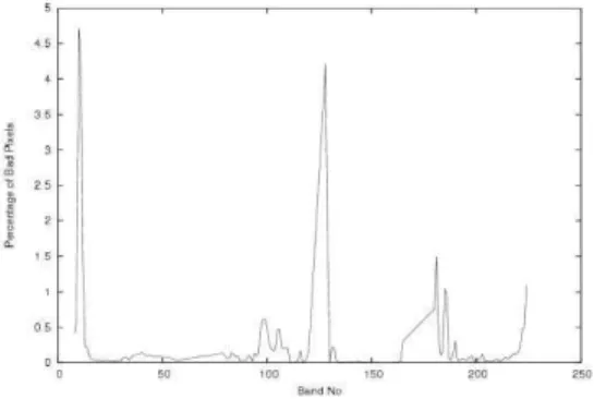
multiple regression coefficients, as explained in the earlier section, were used to generate the soil nutrient images using in-house developed image processing system in Linux. The steps involved are interpolation of the spurious pixel, generation of three spectral derivative images and implementation of coefficient values of the complete image (pixel operation) for six nutrients separately. The geo referenced images of the area of interest in 175 bands were considered. All these images had some spurious pixels, where the reflectance values were either zero or negative. Zero values of the pixel have occurred mostly in deep waters and in the no image area while the negative values were due to overestimation in the atmospheric correction steps. The number of such pixels varied with the wave length (Fig 4). These were first identified and then replaced by using linear interpolation with the good pixels in their immediate vicinity. From the corrected reflectance images, the remaining three derivatives of reflectance images, as discussed in section 4.4, were generated. The regression coefficients obtained from the sample data sets were then used to obtain the nutrient value for every pixel. Six nutrient images were thus generated.
Fig 4 Plot of percent bad pixel versus wavelength
6. RESULTS
6.1 Spectral analysis Spectral feature fitting of the Hyperion
radiance image was done with respect to four likely clay minerals of the area e.g. kaolinite, quartz, illite and montmorillonite. The end member spectra of the minerals were taken from USGS spectral library and compared with the image spectra. The four fit images were converted as point coverage
after appropriate thresholding as follows – illite 4000, kaolinite
2000, montmorrilonite 1500 and quartz 10000. As evident from Fig 5, the area is dominated by quartz mineral followed by illite, kaolinite, and montmorrilonite. The values for thresholding also indicate the relative proportion of the mineral in the soil.
Fig 5 Clay mineral distribution in the study area from SFF analysis
However, northern portion the clay minerals are more dominated by kaolinite compared to illite. The area is dominated by quartz reef, phyllite and schist which after weathering process would likely to yield quartz and koalinitic clay minerals. There are also patches of granite and gneissic lithology in the area that may be contributing to montmorillonitic type of clay minerals.
Pixel purity index analysis was carried out on the reflectance image in order to find out the most pure pixel which can be treated as end member sites to be used for further classification. The PPI image of the study area was further subjected to thresholding with a value of 200. The value was decided with trial and error method with the help of collateral data. The PPI image was converted to vector as point coverage and shows 50 such locations which can be used for further analysis (Fig 6).
Fig 6 PPI locations of the study area
Both these location information after SFF and PPI analysis were used to strategically decide the ground truth sites to be selected in the field for soil sampling and analysis. A total of 58
sites were selected from this analysis for soil sampling but finally 41 sites could be approached in the field due to inadequate approach road (Fig 7). Hand held GPS was used to reach the sites in the field identified from the analysis. Surface soil samples were collected from these 41 sites and used for soil chemical and physico-chemical analysis in the laboratory.
Fig 7 SFF and PPI locations and corresponding ground truth sites
6.2 Soil Chemical Analysis Results of the soil chemical
analysis forty one test sites with respect to six major nutrients and organic carbon in the soil show that the soil is rich in organic carbon (2.53 %) and available potassium (430 Kg/ha) while for available nitrogen and phosphorus, the average values show medium level 336 and 52 Kg/ha respectively. Available calcium, magnesium and sulphur also show a similar trend. Relatively high level of organic carbon (min 1.20 and max 4.65) stems from the fact that the area is primarily hilly terrain. The hills are covered with forest species of trees and are undisturbed soil. The continuous leaf fall during the dormant season gives rise to decomposition and as a result the soil organic carbon percentage in the soil is more than normal soil in the surrounding cultivated area. Available potassium and phosphorus are primarily contributed from the inorganic fraction of the soil. High level of potassium (min 150 and max 905) in the soil indicates that there could be dominance of illite in clay fraction of the soil. The relatively high level of available nitrogen also provides evidence that the soils under the area used for one season during June to November in a year due to lack of irrigation facilities and also the forested terrain might have contributed in the build-up of soil nutrients.
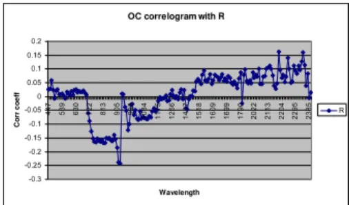
6.3 Statistical Analysis Correlation between spectral value and
nutrient content for all forty-one sites were plotted as a function of spectral wavelength. Correlation were calculated for all four spectral parameter and seven nutrients separately. The spectral band at which the correlation values exceed a threshold value was selected for multiple regression analysis. As a sample the correlogram, Fig 8, e.g. OC vs R has produced eight bands to be used for further analysis with the threshold value of ± 0.15. The bands selected are 762, 813, 905, 915, 925, 2183, 2244, 2345 nm.
Fig 8 Correlogram of organic carbon with four spectral parameters
General trend of the correlograms points out that the variation of the correlation values are more pronounced in case of the derivatives i.e. R’ and A’ compared to R and A. This trend is common for all seven nutrients studied.
Multiple regressions were carried out between the spectral parameters of the selected bands and the soil nutrient content with the sample size of 41 sites. The process was carried out for four spectral parameters and seven nutrients separately
Selection of the spectral parameter was done on the basis of R2,
standard error of prediction SEy , F ratio and RPD. The
parameter having high value of R2, F and RPD and minimum of
error have been selected for calculation of nutrient content of the unknown pixels of the hyperion image.
R’ which is first derivative of reflectance values, was found to
be suitable for estimating the nutrients like OC, N, P and K. A’
which is first derivative of A was found suitable for Ca and S and R was found to be suitable for predicting Mg content in the soil. The parameter A could not perform well for any of the nutrients for prediction purpose. It may be mentioned here that regression process was performed in a recursive manner by dropping those samples where the error component is high and
thereby improving R2. As a result the degrees of freedom (df) is
not same for all the parameters studied in a particular nutrient.
RPD, a measure of standard deviation normalized with SEy ,
was found to be more than 2 in most cases and is defined in category A. Category A models can accurately predict the property in question compared to category B (RPD between 1.4 and 2.0) and category C (RPD less than 1.4) (Chang. and Laird 2002).
After selection of the parameter for each nutrient separately, observed and predicted values were plotted. Best scenario was observed in OC and N while in S prediction would be more realistic in lower values of sulphur content in the soil. For rest of the nutrients the regressive models would likely to perform moderately across the range of nutrient content in the soil. A sample plot between predicted and observed organic carbon is depicted in Fig 9.
6.3 Generation of soil nutrient image Multiple regression
model and the coefficients were used for creating seven soil nutrient images from Hyperion data. The coefficients and the magnitude are different for different nutrients. In other words the number and type of spectral bands used for prediction of different nutrients are different. The minimum and
OC correlogram with R
-0.3 -0.25 -0.2 -0.15 -0.1 -0.05 0 0.05 0.1 0.15 0.2
447 539 630 722 813 905 993 1084 1175 1266 1427 1518 1609 1699 1790 2022 2113 2204 2295 2385
Wavelength
C
o
rr
c
o
e
ff
R
Fig 9 Observed vs Predicted organic carbon
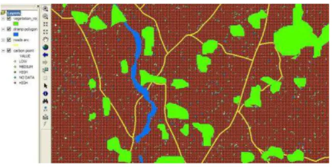
maximum numbers of bands used are 8 and 16 for K and S nutrients respectively. Using these coefficients and R, R1 and A1, as applicable, seven nutrient images were created and a sample OC image is depicted in Fig 10.
Fig 10 Calculated organic carbon from Hyperion
7. CONCLUSIONS
In the present study an attempt has been made to use satellite based hyperspectral data to map soil nutrient status. The basic premise of the study was based on the fact that soil nutrient content is related to soil reflectance or its derivatives at some specified wavelength and the relationship (as regression coefficients) can be extrapolated to estimate the nutrient content of the unknown pixels. The spectral parameter and the wavelength for estimation is nutrient dependent and also may not be universal in nature. But the major advantage in using the Hyperion data was for the selection of soil sampling sites that was carried out based on certain objective criteria. In the traditional practice the selection and soil sampling process in time and cost intensive.
REFERENCES
Ben-Dor E., K. Patkin, A Banin and A. Karnieli 2002, Mapping
of several soil properties using DAIS – 7915 hyperspectral
scanner data – a case study over clayey soils in Israel.
International Journal of Remote Sensing vol.; 23(6)m 1043 –
62.
Chang C.W. and D.A. Laird 2002, Near-infrared reflectance spectroscopic analysis of soil C and N. Soil Science, 167(2), 110-118
Clark, R.N. 1981, The spectral reflectance of water-minreal
mixture at low temperatures. J. Geophys. Res. 86, pp. 3074 – 86
Clark, R.N., G.A. Swayee, N. Gorelick and F.A. Kruse 1991, Mapping with imaging spectrometer data using the complete
band shape lease-square algorithm simultaneously fit to multiple spectral fewatures from multiple materials. Proc of the
third airborne Visible/Infrared Imaging Spectrometer
(AVIRIS), vol 42 2-3, JPL.
Clarke, R.N and T. L. Roush 1984 Reflectance spectroscopy:
Quantitative analysis techniques for remote sensing
applications. Journal of Geophysical Research, 89, 6329 –
6340.
Debba, P., FJA van Ruitenbeek, F.D. van Meer, E.J.M. Carranza and A. Stein 2005, Optimal field sampling for targeting minerals using hyperspectral data. Remote Sensing of
Environment. 99, 373 – 386.
ENVI User’s Guide: Spectral Tools: ENVI version 4.4
FLAASH Module User’s Guide Version 4.3, July, 2006
Jackson, M. L.1973, Soil Chemical Analysis, Prentice – Hall of
India Private Limited, New Delhi. pp. 38 – 56.
Olsen, S. R., C. V. Cole, F. S. Watanabe and L. A. Dean 1954, Estimation of available phosphorus by extraction with sodium bicarbonate. U. S. Dept. Agr. Circ. 939.
Stoner, E.R. and N.F. Baumgardner 1981, Characteristic variations in reflectance of surface soils. Soil Sci. Soc. Am. J.
45, pp. 1161 – 65
Williams, C. H. and A. Steinbergs 1959, Soil sulphur fractions as chemical indices of available sulphur in some Australian
soils. Aust. J. Agric. Res. 10: 340 – 352.
APPENDIX
Category Organic Carbon (%)
Low < 0.50
Medium 0.50 – 0.75
High > 0.75
Category Available Nitrogen (kg N/ha)
Low 200-250
Medium 250-500
High > 500
Observed vs Predicted Soil Organic Carbon (SOC) contents
0.00 1.00 2.00 3.00 4.00 5.00 6.00
0.00 1.00 2.00 3.00 4.00 5.00
SOC contents (% ) observed
S
O
C
c
o
n
te
n
ts
(
%
)
p
re
d
ic
te
d
Low < 28 kg P2O5 ha-1
Medium 28-56 kg P2O5 ha-1
High > 56 kg P2O5 ha-1
Low < 140 kg K2O ha-1
Medium 140 – 280 kg K2O ha-1
High > 280 kg K2O ha-1
Low < 10 ppm av. sulphur
Medium 10 – 20 ppm av. sulphur
High > 20 ppm av. sulphur