www.geosci-model-dev.net/8/1839/2015/ doi:10.5194/gmd-8-1839-2015
© Author(s) 2015. CC Attribution 3.0 License.
Reaching the lower stratosphere: validating an extended vertical
grid for COSMO
J. Eckstein, S. Schmitz, and R. Ruhnke
Karlsruhe Institute of Technology, Institute of Meteorology and Climate Research, Herrmann-von-Helmholtz-Platz 1, 76344 Eggenstein-Leopoldshafen, Germany
Correspondence to:J. Eckstein ([email protected])
Received: 25 November 2014 – Published in Geosci. Model Dev. Discuss.: 26 January 2015 Revised: 6 May 2015 – Accepted: 1 June 2015 – Published: 23 June 2015
Abstract. This study presents an extended vertical grid for the regional atmospheric model COSMO (COnsortium for Small-scale MOdeling) reaching up to 33 km. The extended setup has been used to stably simulate 11 months in a do-main covering central and northern Europe. Temperature and relative humidity have been validated using radiosonde data in polar and temperate latitudes, focussing on the polar and mid-latitude stratosphere over Europe. Temperature values are reproduced very well by the model. Relative humidity could only be met in the mean over the whole time period af-ter excluding data from Russian stations, which showed sig-nificantly higher values. A sensitivity study shows the stabil-ity of the model against different forcing intervals and damp-ing layer heights.
1 Introduction
The upper troposphere and lowermost stratosphere is a place of sharp gradients in many constituents of air and of the phys-ical parameters used to describe its state. Temperature and ozone are textbook examples, but methane, water and many more species also show a strong gradient. At the same time, being the boundary to the lower atmosphere, this is an area where small-scale fluctuations can have a strong influence on the stratosphere and its composition (Zahn et al., 2014).
In order to simulate this highly vulnerable and influ-ential layer directly, a model with high vertical and hori-zontal resolution is needed. Global models usually are too coarsely resolved and cannot model the small-scale pro-cesses. In extending the vertical layering of the regional model COSMO (COnsortium for Small-scale MOdeling) to
33 km, we present here a model that can fill the gap. As we planned to apply the extended setup to simulations covering polar spring and the associated ozone loss with the coupled chemistry model COSMO-ART (COSMO-Aerosols and Re-active Trace gases) (Vogel et al., 2009), we focus here on polar latitudes, but always refer to temperate regions also.
After an introduction to the model and an exact definition of the extended vertical grid in Sect. 2, the measurement data are introduced in Sect. 3. COSMO is shown to be able to run stably with the extended layering. Using radiosonde data and regridded data from meteorological reanalyses, it is shown that the model is able to reproduce temperatures very well (Sect. 4.2) while relative humidity is more difficult (Sect. 4.3) and only its mean value could be reproduced. Two runs with different boundary conditions were performed to test the in-fluence on the model result.
Additionally, three more runs were done in order to test the stability of the model against an increased boundary forcing interval set to 12 and 24 h instead of 6 h and against increas-ing the thickness of the dampincreas-ing layer by settincreas-ing its lower end down to 22 km instead of 28 km. Section 5 presents the results of this sensitivity study, showing that the model will still run stably.
layer difference [m]
height [km]
Level definitions of standard and extended COSMO grid
0 200 400 600 800 1000 1200
0 5 10 15 20 25 30 35
extended grid
damping layer of extended grid standard grid
damping layer of standard grid
Figure 1.The vertical grids of the COSMO model considered in
this study. The damping layers are also given as shaded areas.
2.1 Introduction to the model
COSMO is a regional atmospheric model that has been de-veloped by a consortium lead by the german weather service DWD (German Weather Service). DWD uses the model for its regional numerical weather forecast of Europe and Ger-many with a resolution of 7 and 2.8 km respectively (Baldauf et al., 2011b). Many extensions have been developed for the model, for example COSMO-ART including chemistry and aerosols (Vogel et al., 2009). For this study, the model was set up to run in forecast mode to simulate several months in form of a hindcast using reanalysis data as boundary forcing. The standard setup of COSMO used for the forecast of central Europe (DWD domain COSMO-DE) reaches to a height of 22.0 km (Baldauf et al., 2011a). This is the vertical grid referred to as the standard vertical setup or grid in this study, well aware of the fact the vertical grid used to simu-late a larger European domain (COSMO-EU) that reaches up to 23.6 km (Schulz and Schättler, 2009) is just as frequently used by DWD. The model has also been used to study greater heights in tropical latitudes in the AMMA (African Monsoon Multidisciplinary Analyses) project (Gantner and Kalthoff, 2010), reaching 28.0 km, and a tropical setup reaching up to 30.0 km has also been developed (Krähenmann et al., 2013). With the extended vertical grid presented in this study, it be-comes possible to simulate the lowermost stratosphere in po-lar latitudes. This validation study opens the door to new ap-plications of COSMO.
2.2 The extended vertical grid
The standard vertical grid of the COSMO model reaches up to 22.0 km in 50 layers. The vertical structure is visible in Fig. 1, exact values are given in Table A1. The damping layer in the top layers begins at 11 357 m in standard setup.
layer
height [hPa]
Level definitions of analysis grids
0 10 20 30 40 50 60 70
10−1
100
101
102
103
ERA NCEP
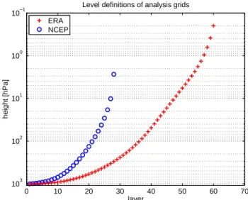
Figure 2.The vertical structure of the NCEP and ERA-Interim
re-analysis used as boundary conditions.
1 2 3
4 5
6 8 7
9 10
11
12 14 1513
16 17 18
19 20 21
22 23
24
90° W 60° W 30° W 0° 30° E 60° E 90° E 30° N
45° N 60° N 75° N
model domain selected stations russian stations polar circle
Figure 3.The model domain and the radiosonde stations used in
this study. The domain is displayed as gray shading, the radiosonde stations are numbered from south to north, numbers also referring to Table B1. Russian stations are marked in red.
The vertical layering of the new grid introduced in this study is also given in Fig. 1 and Table A1. It is focused on the lower stratosphere, with the highest of the 60 layers at 33 km, the damping layer beginning at 28 km (rdheight=28 000.0
in the namelist). The top layer of the extended grid about 10 km above that of the standard grid and the distance be-tween the layers is slightly smaller in all heights above the lowest kilometer, as is also visible in Fig. 1.
z [km]
JAN MAYEN, T during 01.10.2010 to 31.08.2011, sonde data
01.10.10 15.11.10 29.12.10 11.02.11 26.03.11 02.06.11 01.09.11 27
25
23
21
19
17
15
13
11
9
[deg C]
−90 −80 −70 −60 −50 −40 −30
z [km]
JAN MAYEN, T during 01.10.2010 to 31.08.2011, COSMO by ERA
01.10.10 15.11.10 29.12.10 11.02.11 26.03.11 02.06.11 01.09.11 27
25
23
21
19
17
15
13
11
9
[deg C]
−90 −80 −70 −60 −50 −40 −30
Figure 4. Temperature values of all soundings of the station Jan
Mayen, station no. 20. Measurements are displayed on the top, the image below shows the corresponding model values. Note that this is not a time series plot. The dates along the abscissa hold true only for the location they indicate and do not define exact time in be-tween. Dates only increase from left to right, but they are not evenly spaced in time.
(rdheight=22 000.0 in the namelist), which is just the top of
the standard grid. The damping layer then spans one-third of the model layers.
2.3 The analyses used as boundary data
In order to examine the influence of different boundary data on the model results, the model was run twice, using ERA-Interim and NCEP (National Center for Environmental Pre-diction) reanalysis data for starting and boundary values. The vertical layering of the two reanalyses is displayed in Fig. 2. In order to better evaluate the model, the reanalysis data were also interpolated to the vertical grid used for the output of the model.
The reanalysis project of the National Center for Environ-mental Prediction provides data starting on 1 January 1948,
01.10.10 24.11.10 18.01.11 14.03.11 08.05.11 02.07.11 31.08.11 −90
−80 −70 −60 −50 −40 −30
T [deg C]
JAN_MAYEN, T, 26000m, during 01.10.2010 to 31.08.2011
Sonde
COSMO by NCEP COSMO by ERA regridded NCEP regridded ERA
01.10.10 24.11.10 18.01.11 14.03.11 08.05.11 02.07.11 31.08.11 −70
−65 −60 −55 −50 −45 −40
T [deg C]
MADRID, T, 26000m, during 01.10.2010 to 31.08.2011
Sonde
COSMO by NCEP COSMO by ERA regridded NCEP regridded ERA
Figure 5.Time series of measured and modeled temperature, 26 km
above Jan Mayen (top) and Madrid (bottom). Interpolated reanaly-sis data are also shown.
giving global fields every 6 h (00:00, 06:00, 12:00 and 18:00 UTC) at a resolution of T62, which corresponds to 1.875◦(192 points on a latitude) (Kalnay et al., 1996). The
upper boundary is at 2.7 hPa, approximately 42 km in the US standard atmosphere (Sissenwine et al., 1962). So the new vertical grid reaching up to 33 km is still within the vertical limits of the NCEP reanalysis data.
ERA-Interim is the reanalysis project of the European Centre for Medium Range Weather Forecast (ECMWF) (Dee et al., 2011). The data were used in this study at a resolution of T255 (corresponding to 0.7◦, 512 points on a latitude) and
up to 0.1 hPa. So both the vertical and horizontal resolution are higher than those of the NCEP reanalysis. ERA-Interim is available for the same timestamps as the NCEP reanalysis. In standard setup, the reanalysis data were used in a 6-hourly interval (hincbound=6.0 in the namelist) to force
us-ing it as forcus-ing every 12 and 24 h (hincbound=12.0 or
hincbound=24.0 respectively).
2.4 The model domain
The model domain used in this study is shown in Fig. 3. It covers most of Europe with a focus on the polar latitudes, stretching from northern Africa in the south and covering Svalbard, east of Greenland at 74◦N, in the north. The
res-olution was set to 0.2◦. The COSMO model is operationally
used by DWD to produce regional weather forecasts for cen-tral Europe, but not in Northern Hemisphere polar latitudes (Baldauf et al., 2011a).
So the domain chosen here can be used to assess the per-formance of the model in polar latitudes, since a direct com-parison to an area of regular use is possible. The required namelist parameters needed to reproduce the model domain are given in Table A2.
The first time step simulated by the model runs used in this study is 1 October 2010, 00:00 UTC, and the last output is for 1 September 2011, 00:00 UTC. The cold temperatures that can be expected in the polar stratosphere especially in winter and the warming in spring both lay well within the simulated time. Output was produced on an hourly basis, the model time step was set to 60 s, using the namelist parameter dt=60.0. It could be shown that the model runs stably in this
setup by validating the whole time period with radiosonde data.
The timespan of 11 months is due to the time limit ap-plied to the calculation. The model was run with a time limit of 2 days, reaching a total number of 8076 output hours. The last output then turns out to be on 2 September 2011, at 11:00 UTC, but the authors decided to perform this study for the exact 11 months, as given above.
3 Measurements
This study validates the output of the COSMO model using the temperature (T) and relative humidity (RH) recorded by
radiosondes of stations within the model domain.T and RH
are regularly observed values and are here considered basic physical parameters whose distribution well represents the physical state of the model. The measurement data used in this study were taken from the ESRL (Earth System Research Laboratory) radiosonde database provided by NOAA (Na-tional Oceanic and Atmospheric Administration) (Schwartz and Govett, 1992).
The location of the 24 stations is given in Fig. 3, exact values and the names being given in Table B1. This choice includes all polar stations in the domain and the same number of temperate stations with good data coverage.
All stations typically release one radiosonde every 12 h, at 00:00 and 12:00 UTC, so 671 ascents can be expected from each station during the period of 335 simulated days. The
actual number of ascents for each station is also given in Ta-ble B1. All stations except Ny-Ålesund, which has a little more than one ascent per day, come close to or exceed this number, the average being at 673 ascents. Model and regrid-ded reanalysis data were only considered at times when there was an ascent at the specific station, so approximately every 12 h.
In order to compare sonde and model data, the grid point closest to each station was used to compare the simulation with measurements. Since the resolution is only 0.2◦, the
er-ror made by this simple identification is small. The latitude and longitude of the closest grid point can also be found in Table B1. An interpolation to the exact location was not con-sidered necessary as the radiosondes drift with the wind, an effect not accountable, since the exact geographic location of each measurement taken by the sonde is not available. This is also the reason why no interpolation in the vertical was done. In each ascent, the value closest to each model output layer at even kilometers was identified with the height of that layer, the maximum difference allowed having been set to 500 m. Since there are typically more than 20 measurements taken in an ascent, the error was much smaller than this value, reach-ing only 156.0 m on average, with a standard deviation of 126.3 m.
The data were used as downloaded from the server, only excluding values in RH > 100 %. It was found that all stations in Russia give much higher humidity values than the other stations, which is the reason why the humidity data of all Russian stations were excluded from the investigation. This will be further discussed in Sect. 4.3.1.
4 Results
This sections presents the results of the model validation study. Two questions are to be answered: is the model able to simulate the polar latitudes and the stratospheric heights? And what is the influence of the boundary data on these re-sults? Following the questions, the answers will also have to be twofold.
After presenting the output grid, the results in temperature are presented. Those of relative humidity are described in the following section. The latter is preceded by the explanation of why it seemed reasonable to exclude the data of Russian stations when examining relative humidity.
4.1 The output grid
−805 −70 −60 −50 −40 −30 10
15 20 25 30
z [km]
T [deg C]
JAN MAYEN, mean T during 01.10.2010 to 31.08.2011 Sonde COSMO by ERA regridded ERA
−805 −70 −60 −50 −40 −30
10 15 20 25 30
z [km]
T [deg C]
JAN MAYEN, mean T during 01.10.2010 to 31.08.2011 Sonde COSMO by NCEP regridded NCEP
−655 −60 −55 −50 −45 −40 −35 −30 −25 10
15 20 25 30
z [km]
T [deg C]
MADRID, mean T during 01.10.2010 to 31.08.2011 Sonde COSMO by ERA regridded ERA
−655 −60 −55 −50 −45 −40 −35 −30 −25 10
15 20 25 30
z [km]
T [deg C]
MADRID, mean T during 01.10.2010 to 31.08.2011 Sonde COSMO by NCEP regridded NCEP
Figure 6.Mean temperature values at each height for the station on Jan Mayen, station no. 20, on the top, and for Madrid, station no. 1, on
the bottom, showing results of the run forced by ERA-Interim (left) and NCEP (right). The horizontal lines give the 1σstandard deviation.
As noted above, the boundary data were also interpolated onto the output grid, using the same program that is used to prepare the boundary data for running the model, called INT2LM (Schättler, 2013). COSMO uses terrain following coordinates. Above a certain value specified in the namelist, the layers become smooth and are no longer terrain follow-ing. This height has to be higher than the highest mountain tops in the domain and in this case was set to vcflat=7000.0,
given in the namelist in meters. This is the reason why all analyses done in this study only start at 8 km.
4.2 Temperature
To begin the discussion, a look at Fig. 4 exemplifies the ba-sis of this study. It shows all the soundings of the station Jan Mayen during the time considered here. The warming at the end of the polar winter can be plainly seen. Most striking are the many white areas in the image, showing the lack of mea-surement data. The bottom figure shows the corresponding result of the model run with boundary data by ERA-Interim. The image is filled, but the data were only used for the fol-lowing analysis if measurements were also available at the timestamp.
Figure 5 gives exemplary time series of Jan Mayen and Madrid at 26 km height, approximately 2.5 km above the model top of the standard vertical COSMO grid for both model runs. When comparing the two figures, tempera-ture values reflect the different latitude: winter temperatempera-tures above Jan Mayen are much colder than above Madrid, the warming in spring much more pronounced. The good corre-spondence of model and measurement not only shows that the two model runs and also the boundary data are very sim-ilar, but also that the model performance does not change during the whole simulated period. There is no greater offset in the end than in the beginning.
To compare the data in a more quantitative manner, Fig. 6 shows the mean ascent at Jan Mayen for both model runs. The boundary data are also included in the image. All three soundings lay on top of each other. The minimum temper-ature in the lowermost stratosphere is well reproduced. In order to compare to a temperate station, Fig. 6 also gives the mean ascent of the station in Madrid. The minimum is more pronounced, but also reproduced by the model. There is no difference visible between the model run forced by ERA-Interim and that forced by NCEP reanalysis data.
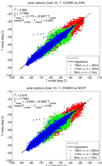
mod-Figure 7. Scatterplot of modeled against measured temperature
for polar stations when forcing the model with ERA-Interim (top) and NCEP reanalysis data (bottom). The data were color coded by height to visually inspect the variability in each height section. The statistics in the upper left hand corner refer to the whole data set.
eled temperature values with color coded height intervals for all polar stations. The variability in higher altitudes is lower, which is why the scatter is reduced with height. Both model runs with different boundary data simulate temperature very well, reaching aboutr2=0.98. The results of the model in
temperate latitudes was just as good and the correlation does not reach higher values when using the regridded boundary data (not shown).
When reducing the data to values of descriptive statistics, all stations can be easily compared. Figure 8 shows the mean
of Tmodel−Tmeas and Tbound−Tmeas for all levels and for
stratospheric levels withz≥11 km. The stratospheric layers
are also those layers added when using the extended instead of the standard vertical grid. In both cases, the values are well reproduced by the model. When considering all layers, the mean values of the boundary data are lower than those of
2 4 6 8 10 12 14 16 18 20 22 24
−3 −2.5 −2 −1.5 −1 −0.5 0 0.5 1 1.5 2
station number
mean(
∆
T)
mean(∆T) during 01.10.10 to 31.08.11 for all levels
<< temperate polar >>
ERA: COSMO−meas NCEP: COSMO−meas ERA: regridded−meas NCEP: regridded−meas
2 4 6 8 10 12 14 16 18 20 22 24
−2 −1.5 −1 −0.5 0 0.5 1 1.5
station number
mean(
∆
T)
mean(∆T) during 01.10.10 to 31.08.11 for z >=11000m
<< temperate polar >>
ERA: COSMO−meas NCEP: COSMO−meas ERA: regridded−meas NCEP: regridded−meas
Figure 8.Mean difference in temperature over all heights (top) and
heights withz≥11 km (bottom) for each station. The dashed line
corresponds in color to the full line which is always half the standard deviation of the difference above and below the mean value. See Table B1 for a list of the stations corresponding to the numbers.
measurement, the model output actually being closer to the measurement. When considering the new stratospheric lay-ers, the model performance is just as good as it is when con-sidering all layers. The boundary data are now closer to mea-surements than for all levels. Overall, COSMO is able to re-produce measurements in temperate as well as polar latitudes in all heights, the mean difference never exceeding 0.5 K.
1 2 3 4 5
6 8 7
9 10 11
12 14 1513 16 17 18
19 20 21
22 23
24
Meas−COSMO by ERA, 01.10.10 to 31.08.11, all levels
60° W 30° W 0° 30° E 60° E 90° E 30° N
45° N 60° N 75° N
∆ T [K]
−0.6 −0.4 −0.2 0 0.2
Figure 9.Mean difference of model values and measurements of
temperature for each station over all levels when using ERA-Interim as forcing data. The picture is similar when using NCEP reanalysis data.
the relative location of the three stations within the model domain but more likely to the measurement data.
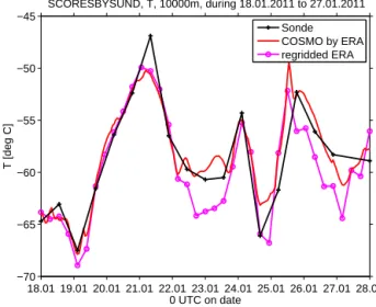
Another aspect when comparing the model output to mea-surements and regridded reanalysis data are the variability of the model in between those times when measurements or reanalysis data are available. Model output was saved every hour, while measurement or reanalysis data are available at most every 6 h, as explained in Sects. 2.3 and 3. In order to asses this variability, Fig. 10 shows a shorter time series of only 10 days of the three data sets, including all existing model and reanalysis data. It becomes obvious that the model shows an internal variability that is not present in the less frequent measurement or reanalysis data. The greater vari-ability is linked to physical processes that happen on short timescales of only hours or less. These cannot be captured by regridding the reanalysis data to a finer grid.
4.3 Relative humidity
4.3.1 Excluding the Russian humidity data
When examining the relative humidity of the 24 stations cho-sen for the validation of the model, it became apparent that the model could not reproduce the relative humidity data of any station within Russia (or of Gomel, the only station in Belarus with data during the modeled period, as became clear when examining more stations).
As there was no apparent reason for this offset and only seven stations lay within Russia in the original set (five polar and two temperate), this issue needed further investigation. The data of all available 23 Russian stations well within the model domain and Gomel in Belarus (see Table B2) were
18.01 19.01 20.01 21.01 22.01 23.01 24.01 25.01 26.01 27.01 28.01 −70
−65 −60 −55 −50 −45
0 UTC on date
T [deg C]
SCORESBYSUND, T, 10000m, during 18.01.2011 to 27.01.2011
Sonde COSMO by ERA regridded ERA
18.01 19.01 20.01 21.01 22.01 23.01 24.01 25.01 26.01 27.01 28.01 −68
−66 −64 −62 −60 −58 −56 −54 −52
0 UTC on date
T [deg C]
SCORESBYSUND, T, 23000m, during 18.01.2011 to 27.01.2011
Sonde COSMO by ERA regridded ERA
Figure 10.Time series of measured and modeled temperature as
well as the regridded boundary data, 10 (top) and 23 km (bottom) above Scoresbysund, station no. 19, over 10 days at the end of Jan-uary 2011. All data points available in each data set are included.
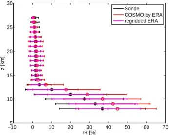
compared with 24 other stations in the eastern part of the do-main but not in Russia or Belarus (see Table B3). The result is best illustrated by the mean over all RH values of all as-cents in each group. Figure 11 shows the result for the Rus-sian stations and the 24 stations outside of Russia that had been chosen. While the model reproduces the values of the stations outside of Russia, the measurement values of those stations within Russia are very different from the model val-ues but also from the regridded analysis or the measurements of those stations outside of Russia.
−105 0 10 20 30 40 50 60 70 10
15 20 25 30
z [km]
rH [%]
russian stations (total 24), mean rH during 01.10.2010 to 31.08.2011
Sonde COSMO by ERA regridded ERA
−105 0 10 20 30 40 50 60 70
10 15 20 25 30
z [km]
rH [%]
nonrussian stations (total 24), mean rH during 01.10.2010 to 31.08.2011
Sonde COSMO by ERA regridded ERA
Figure 11.Mean relative humidity values of Gomel (BY) and the
23 Russian stations (top), and 24 stations outside of Russia but in the eastern part of the domain (bottom). The horizontal lines give
the 1σstandard deviation.
These two findings are in line with Balagurov et al. (2006) and Moradi et al. (2013). The authors of these studies come to the conclusion that the measurement technique used in ra-diosondes of Russia give values for relative humidity that are significantly too high for low pressure. All together, this lead to the decision to exclude Russian stations from the further investigation of the performance of COSMO with respect to relative humidity.
4.3.2 Results when excluding Russian data
When excluding the Russian stations (no. 7, 10, 13, 16–18 and 21), 10 temperate and 7 polar stations remain to examine relative humidity.
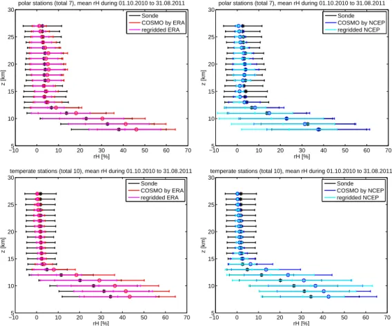
The mean values of the ascents of temperate and polar sta-tions for both model runs is given in Fig. 12. The low
strato-spheric values are well reproduced by the model for polar and temperate stations and both runs, while the tropospheric offset is larger. In heights lower than 13 km, the model is too humid on average, the values being approximately 10 % too high. The mean of tropospheric values seems to be better reproduced for polar stations when using the NCEP reanal-ysis. The bias is of measurements and model data are also present in the forcing reanalysis data, these being dryer than measurements on average. The model reduces this bias and produces a wetter atmosphere than that of the reanalyses. So the bias is combination of model physics, boundary data and maybe also measurement problems. Overall, model results fit measurements better than the reanalysis data.
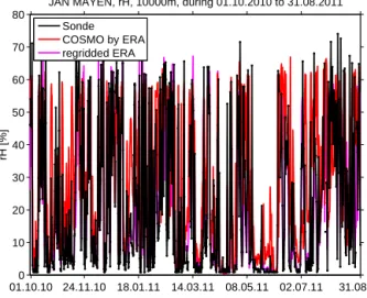
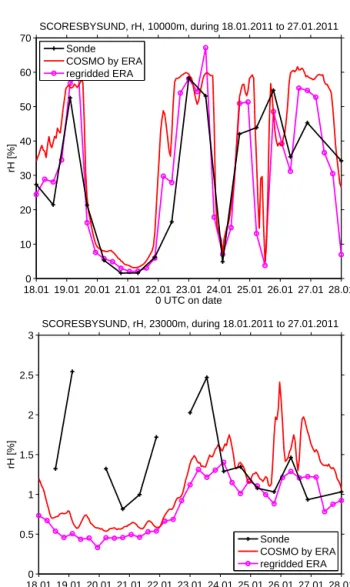
However, when looking at the scatterplot of the polar sta-tions, given in Fig. 13, it becomes clear that the model is only able to reproduce a mean value that is similar to the measurements. There is no notable correlation in any height. The variability in the measurements is simply too high to be reproduced by the model. This is also visible in the fig-ures showing the mean ascents. The standard deviation of the model and the regridded analysis is much smaller than that of the measurements in stratospheric layers. Figure 14 shows the time series of relative humidity at 10 and 21 km heights. At 21 km height, the values are very low most of the time. While the small-scale variations in the troposphere are not reproduced by the model, the stratospheric variability is well captured by the model.
Figure 15 shows the spatial distribution of mean RHmeas−
RHmodel over all layers. The Russian stations have been
ex-cluded, but two other stations also show an offset compared to the other stations: Tórshavnar (no. 11) and Scoresbysund (no. 23). The modeled values are higher than measurements, with1RH=4 %. This again is probably not an effect of the
model but more likely of the measurements since surround-ing stations do not show similar effects. The value fits the range of 2–6 % of dry bias reported by Wang et al. (2013) for radiosondes of type Vaisala RS92, but the type of sonde is not known for any of the stations in this study.
Relative humidity is on the one side very variable, so that it becomes hard to model exactly, and on the other side it seems not an easy parameter to measure, as the problems first found in Russian data show which are apparently also present in the data of other stations.
−105 0 10 20 30 40 50 60 70 10
15 20 25 30
z [km]
rH [%]
polar stations (total 7), mean rH during 01.10.2010 to 31.08.2011
Sonde COSMO by ERA regridded ERA
−105 0 10 20 30 40 50 60 70 10
15 20 25 30
z [km]
rH [%]
polar stations (total 7), mean rH during 01.10.2010 to 31.08.2011
Sonde COSMO by NCEP regridded NCEP
−105 0 10 20 30 40 50 60 70 10
15 20 25 30
z [km]
rH [%]
temperate stations (total 10), mean rH during 01.10.2010 to 31.08.2011
Sonde COSMO by ERA regridded ERA
−105 0 10 20 30 40 50 60 70 10
15 20 25 30
z [km]
rH [%]
temperate stations (total 10), mean rH during 01.10.2010 to 31.08.2011
Sonde COSMO by NCEP regridded NCEP
Figure 12.Mean values of relative humidity for polar (top) and temperate (bottom) stations for the model run forced by ERA-Interim (left)
an NCEP (right) reanalysis data. Russian stations were excluded from this analysis, as described in the text. The horizontal lines give the 1σ
standard deviation.
so large that the model cannot be expected to reproduce the exact values that were measured at a specific site.
5 Sensitivity study
5.1 Boundary forcing interval
This section describes the results of the two model runs that were performed with larger boundary forcing intervals of 12 h (called int12 in plots) and 24 h (int24) relative to the other runs with 6-hourly forcing (called int6). Both of these runs ran stably and the setups were used to simulate the same time period as the run with 6-hourly forcing.
In order to compare the three runs, Table C1 gives the cor-relation coefficients of model and measured temperature and relative humidity (excluding Russian stations) for all three runs, listed separately for polar and temperate stations. The correlation is slightly weaker for both variables with the in-creased boundary forcing interval, the coefficient becoming smaller as the interval increases. This is expected, as the forc-ing interval determines how strongly the model is influenced by the boundary values that represent a realistic meteorology. But the decrease is not very strong and measured temperature
can still be seen as very well reproduced even by the run that uses only one boundary input field per day.
In addition to comparing each run with measurement data, the runs can be directly compared with one another. For this, the 6-hourly time series data that was prepared at each station presents a good database. The difference between the model runs does not increase with simulation time (not shown). The mean difference between the separate stations and a mean of all stations in each height is presented in Fig. 17. In all heights and for both variables, the run with 24-hourly forcing shows a larger difference to the original run than the run with 12-hourly forcing.
5.2 Extending the damping layer
In a second test, the sensitivity of the model to the extent of the damping layer was investigated with an additional model run. For this run, the lower end of the damping layer was set to 22 km (called rdh22 in plots), 6 km lower than in the original run (rdh28). It then extends one-third of total model height of 33 km.
insta-Figure 13. Scatterplots of modeled against measured relative
hu-midity for the runs forced by ERA-Interim (top) and NCEP (bot-tom). The data were color coded by height to visually inspect the variability in each height section. The statistics in the upper left hand corner refer to the whole data set.
bilities lead to the breakdown of the model. The reasons for these instabilities were not investigated further, but this also showcases that it is not a trivial task to find a vertical grid with which the model runs stably.
The setup with rdheight=22.0 on the other hand ran
sta-bly for the time period considered in this study. Table C2 lists the correlation coefficient of model against measurement data for temperate and polar stations, including all layers up to 21 km. The differences are only marginally small and the runs can be considered to reproduce measurements equally well.
In order to asses the difference between the model runs, the 6-hourly data generated for each station are again used to calculate a profile of the difference of the two model runs for each station and for the whole data set. The result of the analysis is shown in Fig. 18. The shapes of the curves are
01.10.10 24.11.10 18.01.11 14.03.11 08.05.11 02.07.11 31.08.11 0
10 20 30 40 50 60 70 80
rH [%]
JAN MAYEN, rH, 10000m, during 01.10.2010 to 31.08.2011
Sonde COSMO by ERA regridded ERA
01.10.10 24.11.10 18.01.11 14.03.11 08.05.11 02.07.11 31.08.11 0
10 20 30 40 50 60
rH [%]
JAN MAYEN, rH, 21000m, during 01.10.2010 to 31.08.2011
Sonde COSMO by ERA regridded ERA
Figure 14.Time series of relative humidity at 10 km (top) and
21 km (bottom) height above Jan Mayen for the model forced by ERA-Interim data.
similar to those of Fig. 17, where the boundary input inter-val was varied. The overall difference is small and similar in magnitude to the difference when doubling the boundary forcing interval to 12 h. Just where the damping layer starts to be active, a kink is visible in the profile ofT, showing the
necessity to stop evaluation of the model below the damping layer height when wanting to compare measurements and the model.
6 Summary and conclusions
1 2 3 4 5
6 8 7
9 10 11
12 14 1513 16 17 18
19 20 21
22 23
24
Meas−COSMO by ERA, 01.10.10 to 31.08.11, all levels
60° W 30° W 0° 30° E 60° E 90° E 30° N
45° N 60° N 75° N
∆ rH [%]
−4 −2 0 2 4
Figure 15.Mean difference of measurements and model values of
relative humidity for each station when using ERA-Interim as forc-ing data. The picture is similar when usforc-ing NCEP reanalysis data.
to 11 km in the standard setup. This is already well in the lowermost stratosphere.
The extended vertical grid is planned to be used for sim-ulations covering the polar spring and the associated ozone loss, which is why it was tested using a domain spread-ing over central and northern Europe. To assess the in-fluence of different boundary conditions, two model runs were compared with measurements, using ERA-Interim or NCEP reanalysis as boundary conditions for the model. Both model runs covered the same period, from 1 October 2010 to 1 September 2011. The model simulated this period stably. Additionally, three more runs using ERA-Interim as bound-ary forcing were done, two with increased boundbound-ary forcing intervals of 12 and 24 h and one with an increased damping reaching down to 22 km.
The output was compared with measurements of tempera-ture and relative humidity from all 12 polar radiosonde sta-tions in the domain and as many in temperate latitudes.
The measurements of temperatures are well reproduced by the model for all stations and heights. This is not only true for the mean, but also for the comparison of single ascents. The error in heights above 11 km is even smaller than that when considering all layers, probably because the variability is not as high as when including the tropospheric values. The mean error made by the model is smaller than 0.5 K for all stations. The boundary data, which was regridded to the output grid, reaches similar values.
When comparing relative humidity values, it was found that Russian stations (and Gomel in Belarus) had system-atically submitted higher values. This finding was strength-ened by comparing all 23 Russian stations in the domain and Gomel to 24 stations not in Russia but in the eastern part of
18.01 19.01 20.01 21.01 22.01 23.01 24.01 25.01 26.01 27.01 28.01 0
10 20 30 40 50 60 70
0 UTC on date
rH [%]
SCORESBYSUND, rH, 10000m, during 18.01.2011 to 27.01.2011
Sonde COSMO by ERA regridded ERA
18.01 19.01 20.01 21.01 22.01 23.01 24.01 25.01 26.01 27.01 28.01 0
0.5 1 1.5 2 2.5 3
0 UTC on date
rH [%]
SCORESBYSUND, rH, 23000m, during 18.01.2011 to 27.01.2011
Sonde COSMO by ERA regridded ERA
Figure 16.Time series of relative humidity at 10 (top) and 23 km
(bottom) heights above Scoresbysund for the model, the forcing ERA-Interim reanalysis and the measurement data at the end of Jan-uary 2011.
the domain and considering model and boundary data. After excluding Russian stations from the analysis of relative hu-midity, it became apparent that the model is not capable of re-producing the exact values of each measurement and neither is the regridded boundary data. But it does reproduce the low stratospheric values and fits measurements well when taking a mean over the whole time period. In the tropospheric lay-ers, the model values are more humid than measurements.
0 0.5 1 1.5 2 2.5 3 3.5 8
10 12 14 16 18 20 22 24 26 28
T, abs(int6−int12) and abs(int6−int24)
absolute difference [K]
height [km]
stations int6−int12 mean int6−int12 stations int6−int24 mean int6−int24
0 5 10 15 20
8 10 12 14 16 18 20 22 24 26 28
rH, abs(int6−int12) and abs(int6−int24)
absolute difference [%]
height [km]
stations int6−int12 mean int6−int12 stations int6−int24 mean int6−int24
Figure 17. Difference between the model runs with 12 and
24-hourly forcing to the original run with 6-24-hourly forcing forT (top)
and RH (bottom). Shown is one profile for each station and the mean of all stations.
The height of the damping layer does influence the results of the model, but differences reach only about 1 K to the case of
T, for example.
The vertical grid for COSMO presented in this study seems a good alternative to the standard vertical layering of the COSMO-DE domain when focusing on the upper tropo-sphere and lower stratotropo-sphere in polar latitudes. It has been shown to run stably, simulating almost a year. By comparing with data from synoptic radiosondes and regridded reanaly-sis data, it could be shown that the model is able to reproduce measurements of temperature well and produce reasonable values of relative humidity. The enlarged time series show a small-scale variability in the model that is not present in the measurements and cannot be expected form regridding the boundary data. The stability against varying the bound-ary forcing interval and the extent of the damping layer was
0 0.5 1 1.5 2
8 10 12 14 16 18 20 22 24 26 28
T, abs(rdh28−rdh22)
absolute difference [K]
height [km]
stations rdh28−rdh22 mean rdh28−rdh22 damping layer start
0 2 4 6 8 10 12 14
8 10 12 14 16 18 20 22 24 26 28
rH, abs(rdh28−rdh22)
absolute difference [%]
height [km]
stations rdh28−rdh22 mean rdh28−rdh22 damping layer start
Figure 18.Difference between the model run with the lowest extent
of the damping layer at 28 km to the standard with rdheight=22 for
T (top) and RH (bottom). Shown is one profile for each station and
the mean of all stations.
Appendix A: Model specifications
This appendix specifies the model setup. It gives the namelist settings for the preprocessor int2lm needed to reproduce the geographic model domain in Table A2 and the exact values of the vertical grids – the new, extended grid as well as the standard grid used for COSMO-DE – in Table A1.
Table A1.Heights of the layers of the standard and the extended
COSMO grid, specified in meters.
No. Extended Standard No. Extended Standard
0 0.00 0.00 31 8711.53 7539.64
1 70.00 20.00 32 9255.31 8080.00
2 151.86 51.43 33 9818.03 8642.86
3 245.82 94.64 34 10 399.91 9228.57
4 352.10 150.00 35 11 001.17 9837.50
5 470.92 217.86 36 11 622.05 10 470.00
6 602.52 298.57 37 12 262.76 11 126.43
7 747.13 392.50 38 12 923.55 11 807.14
8 904.97 500.00 39 13 604.64 12 512.50
9 1076.27 621.43 40 14 306.25 13 242.86
10 1261.25 757.14 41 15 028.62 13 998.57
11 1460.15 907.50 42 15 771.97 14 780.00
12 1673.20 1072.28 43 16 536.53 15 587.50
13 1900.61 1253.57 44 17 322.52 16 421.43
14 2142.63 1450.00 45 18 130.19 17 282.14
15 2399.47 1662.50 46 18 959.74 18 170.00
16 2671.37 1891.43 47 19 811.42 19 085.36
17 2958.56 2137.14 48 20 685.45 20 028.57
18 3261.25 2400.00 49 21 582.05 21 000.00
19 3579.68 2680.36 50 22 501.46 22 000.00
20 3914.09 2978.57 51 23 443.90 –
21 4264.68 3295.00 52 24 409.61 –
22 4631.70 3630.00 53 25 398.80 –
23 5015.37 3983.93 54 26 411.71 –
24 5415.92 4357.14 55 27 448.57 –
25 5833.58 4750.00 56 28 509.60 –
26 6268.57 5162.86 57 29 595.03 –
27 6721.12 5596.07 58 30 705.08 –
28 7191.47 6050.00 59 31 840.00 –
29 7679.83 6525.00 60 33 000.00 –
30 8186.44 7021.43 – – –
Table A2.Name list parameters of the preprocessor int2lm needed
to reproduce the model domain.
Name list block Parameter Value
LMGRID ivctype 2
irefatm 2
lnewVGrid .TRUE.
ielm_tot 190
jelm_tot 255
kelm_tot 60
pollat 30.0
pollon −170.0
polgam 0.0
dlon 0.2
dlat 0.2
startlat_tot −29.0
startlon_tot −19.0
vcflat 18 000.0
DATA ie_ext 200
Appendix B: Specifications of the stations
This appendix specifies the stations from which data were used in this study. Table B1 lists the information for those stations used for the original study, while Tables B2 and B3 list the information of the 48 stations that were used to inves-tigate the bias in relative humidity of the stations in Russia.
Table B1.Specifications of the stations from which data were used in this study. Stations 1–12 are in temperate latitudes, 13–24 in polar
latitudes. The international country code is also given. Real coordinates are those of the true location, model coordinates those of the closest grid point used to compare measurements and model data.
No. Name Country WMO no. Lat real Lat model Long real Long model Ascents
1 Madrid ES 08221 40.470 40.494 −3.580 −3.521 654
2 Pratica di Mare IT 16245 41.650 41.562 12.430 12.537 995
3 Bucharest RO 15420 44.500 44.554 26.130 26.168 670
4 Stuttgart DE 10739 48.830 48.796 9.200 9.107 674
5 Legionowo PL 12374 52.400 52.428 20.970 21.112 671
6 Castor Bay IE 03918 54.300 54.247 −6.190 −6.178 495
7 Moscow RU 27612 55.750 55.859 37.570 37.458 633
8 Stavanger SE 01415 58.870 58.929 5.670 5.735 623
9 Jokioinen FI 02963 60.820 60.721 23.500 23.588 652
10 Kargopol RU 22845 61.500 61.441 38.930 38.903 593
11 Tórshavnar DK 06011 62.020 62.007 −6.770 −6.783 651
12 Keflavik IS 04018 63.970 63.951 −22.600 −22.593 649
13 Kandalaksha RU 22217 67.150 67.136 32.350 32.366 670
14 Bodo Vi NO 01152 67.250 67.137 14.400 14.601 651
15 Sodankylä FI 02836 67.370 67.390 26.650 26.677 663
16 Naryan Mar RU 23205 67.650 67.662 53.020 52.948 636
17 Sojna RU 22271 67.880 67.946 44.130 44.126 650
18 Murmansk RU 22113 68.970 68.963 33.050 33.004 672
19 Scoresbysund GL 04339 70.480 70.642 −21.970 −22.020 657
20 Jan Mayen NO 01001 70.930 70.911 −8.670 −8.860 1040
21 Malye Karmakuly RU 20744 72.380 72.285 52.730 52.609 591
22 Bjørnøya NO 01028 74.520 74.640 19.020 18.792 986
23 Danmarkshavn GL 04320 76.770 76.759 −18.670 −18.470 644
Table B2.Specifications of the Russian stations from which data were used in this study, listed from south to north. Real coordinates are
those of the true location, model coordinates those of the closest grid point used to compare measurements and model data.
No. Name Country WMO no. Lat real Lat model Long real Long model Ascents
1 Voronez RU 34122 51.670 51.608 39.270 39.392 640
2 Kursk RU 34009 51.770 51.865 36.170 36.056 603
3 Gomel BY 33041 52.450 52.595 31.000 30.948 468
4 Suhinici RU 27707 54.120 53.983 35.330 35.341 587
5 Ryazan RU 27730 54.630 54.651 39.700 39.578 668
6 Kaliningrad RU 26702 54.700 54.696 20.620 20.733 442
7 Smolensk RU 26781 54.750 54.680 32.070 32.131 671
8 Moscow RU 27612 55.750 55.859 37.570 37.458 633
9 Nizhny Novgorod RU 27459 56.270 56.330 44.000 43.869 654
10 Velikie Luki RU 26477 56.380 56.450 30.600 30.566 649
11 Bologoye RU 26298 57.900 57.877 34.050 34.220 639
12 Vologda RU 27037 59.230 59.217 39.870 39.908 300
13 St. Petersburg RU 26063 59.970 60.054 30.300 30.348 656
14 Kargopol RU 22845 61.500 61.441 38.930 38.903 593
15 Syktyvkar RU 23804 61.720 61.672 50.830 50.748 668
16 Petrozavodsk RU 22820 61.820 61.926 34.270 34.313 666
17 Arhangelsk RU 22550 64.530 64.405 40.580 40.568 296
18 Kem RU 22522 64.980 65.083 34.800 34.658 645
19 Pecora RU 23418 65.120 65.044 57.100 57.081 670
20 Kandalaksha RU 22217 67.150 67.136 32.350 32.366 670
21 Naryan Mar RU 23205 67.650 67.662 53.020 52.948 636
22 Sojna RU 22271 67.880 67.946 44.130 44.126 650
23 Murmansk RU 22113 68.970 68.963 33.050 33.004 672
24 Malye Karmakuly RU 20744 72.380 72.285 52.730 52.609 589
Table B3.Same as Table B2 but for those stations outside of Russia used to compare to those in Russia.
No. Name Country WMO no. Lat real Lat model Long real Long model Ascents
1 Bucharest RO 15420 44.500 44.554 26.130 26.168 670
2 Cluj Napoca RO 15120 46.780 46.839 23.570 23.496 336
3 Poprad PL 11952 49.030 49.073 20.320 20.240 672
4 Prostejov PL 11747 49.450 49.337 17.130 17.256 656
5 Prague CZ 11520 50.000 49.896 14.450 14.589 1341
6 Wroclaw PL 12425 51.130 51.169 16.980 16.949 668
7 Lin DE 10393 52.220 52.118 14.120 14.197 1348
8 Legionowo PL 12374 52.400 52.428 20.970 21.112 671
9 Greifswald DE 10184 54.100 54.149 13.400 13.399 668
10 Schleswig DE 10035 54.530 54.599 9.550 9.656 671
11 Leba PL 12120 54.750 54.747 17.530 17.609 667
12 Kaunas LT 26629 54.880 54.757 23.880 23.914 336
13 Visby SE 02591 57.650 57.725 18.350 18.255 594
14 Gothenburg SE 02527 57.670 57.580 12.300 12.237 331
15 Stavanger NO 01415 58.870 58.929 5.670 5.735 623
16 Tallinn EE 26038 59.450 59.574 24.800 24.733 333
17 Jokioinen FI 02963 60.820 60.721 23.500 23.588 652
18 Jyväskylä FI 02935 62.400 62.346 25.670 25.642 670
19 Sundsvall SE 02365 62.530 62.610 17.470 17.398 598
20 Ørland NO 01241 63.700 63.599 9.600 9.551 667
21 Luleå SE 02185 65.550 65.542 22.130 22.085 331
22 Bodo Vi NO 01152 67.250 67.137 14.400 14.601 638
23 Sodankylä FI 02836 67.370 67.390 26.650 26.677 663
Appendix C
Table C1.Correlation coefficients for the three model runs forced by ERA-Interim against measurements, using 6-, 12- or 24-hourly boundary
forcing for polar and temperate stations and both variables,T and RH.
Temperate Polar
Forcing
interval 6 12 24 6 12 24
T 0.961 0.957 0.946 0.982 0.979 0.973
RH 0.754 0.740 0.707 0.747 0.735 0.706
Table C2.Correlation coefficients for the two model runs forced by ERA-Interim against measurements, using 28 or 22 km as lowest extents
of the damping layer for polar and temperate stations and both variables,T and RH.
Temperate Polar
Damp. height 28 22 28 22
T 0.961 0.962 0.982 0.982
Acknowledgements. We acknowledge support by Deutsche Forschungsgemeinschaft and Open Access Publishing Fund of Karlsruhe Institute of Technology.
The article processing charges for this open-access publication were covered by a Research
Centre of the Helmholtz Association.
Edited by: A. Kerkweg
References
Balagurov, A., Kats, A., Krestyannikova, N., and Schmidlin, F.: WMO Radiosonde humidity sensor intercomparison, Instru-ments and observing methods report No. 85 WMO/TD-No. 1305, WMO, Geneva, Switzerland, 2006.
Baldauf, M., Förstner, J. F., Klink, S., Reinhardt, T., Schraff, C., Seifert, A., and Stephan, K.: Kurze Beschreibung des Lokal-Modells Kürzestfrist COSMO-DE (LMK) und seiner Daten-banken auf dem Datenserver des DWD, Tech. rep., DWD, Of-fenbach, Germany, 2011a.
Baldauf, M., Seifert, A., Förstner, J., Majewski, D., Raschendor-fer, M., and Reinhardt, T.: Operational convective-scale numeri-cal weather prediction with the COSMO model: description and sensitivities, Mon. Weather Rev., 139, 3887–3905, 2011b. Dee, D. P., Uppala, S. M., Simmons, A. J., Berrisford, P., Poli,
P., Kobayashi, S., Andrae, U., Balmaseda, M. A., Balsamo, G., Bauer, P., Bechtold, P., Beljaars, A. C. M., van de Berg, L., Bid-lot, J., Bormann, N., Delsol, C., Dragani, R., Fuentes, M., Geer, A. J., Haimberger, L., Healy, S. B., Hersbach, H., Hólm, E. V., Isaksen, L., Kållberg, P., Köhler, M., Matricardi, M., McNally, A. P., Monge-Sanz, B. M., Morcrette, J.-J., Park, B.-K., Peubey, C., de Rosnay, P., Tavolato, C., Thépaut, J.-N., and Vitart, F.: The ERA-Interim reanalysis: configuration and performance of the data assimilation system, Q. J. Roy. Meteorol. Soc., 137, 553– 597, doi:10.1002/qj.828, 2011.
Gantner, L. and Kalthoff, N.: Sensitivity of a modelled life cycle of a mesoscale convective system to soil conditions over West Africa, Q. J. Roy. Meteorol. Soc., 136, 471–482, doi:10.1002/qj.425, 2010.
Kalnay, E., Kanamitsu, M., Kistler, R., Collins, W., Deaven, D., Gandin, L., Iredell, M., Saha, S., White, G., Woollen, J., Zhu, Y., Leetmaa, A., Reynolds, R., Chelliah, M., Ebisuzaki, W., Higgins, W., Janowiak, J., Mo, K. C., Ropelewski, C., Wang, J., Jenne, R., and Joseph, D.: The NCEP/NCAR 40-Year Reanalysis Project, B. Am. Meteorol. Soc., 77, 437–471, 1996.
Krähenmann, S., Kothe, S., Panitz, H.-J., and Ahrens, B.: Eval-uation of daily maximum and minimum 2-m temperatures as simulated with the Regional Climate Model COSMO-CLM over Africa, Meteorol. Z., 22, 297–316, doi:10.1127/0941-2948/2013/0468, 2013.
Moradi, I., Soden, B., Ferraro, R., Arkin, P., and Vömel, H.: As-sessing the quality of humidity measurements from global oper-ational radiosonde sensors, J. Geophys. Res.-Atmos., 118, 8040– 8053, doi:10.1002/jgrd.50589, 2013.
Schättler, U.: A Description of the Nonhydrostatic Regional COSMO-Model Part V: Preprocessing: Initial and Boundary Data for the COSMO-Model, Tech. rep., DWD, Offenbach, Ger-many, 2013.
Schulz, J.-P. and Schättler, U.: Kurze Beschreibung des Lokal-Modells Europa COSMO-EU (LME) und seiner Datenbanken auf dem Datenserver des DWD, Tech. rep., DWD, Offenbach, Germany, 2009.
Schwartz, B. and Govett, M.: A Hydrostatically Consistent North American Radiosonde Data Base At The Forecast Systems oratory, 1946–Present, Tech. rep., NOAA, Forecast Systems Lab-oratory, Boulder, USA, 1992.
Sissenwine, N., Dubin, M., and Wexler, H.: The U.S. Stan-dard Atmosphere, 1962, J. Geophys. Res., 67, 3627–3630, doi:10.1029/JZ067i009p03627, 1962.
Vogel, B., Vogel, H., Bäumer, D., Bangert, M., Lundgren, K., Rinke, R., and Stanelle, T.: The comprehensive model system COSMO-ART – Radiative impact of aerosol on the state of the atmo-sphere on the regional scale, Atmos. Chem. Phys., 9, 8661–8680, doi:10.5194/acp-9-8661-2009, 2009.
Wang, J., Zhang, L., Dai, A., Immler, F., Sommer, M., and Vömel, H.: Radiation dry bias correction of Vaisala RS92 humidity data and its impacts on historical radiosonde data, J. Atmos. Ocean. Tech., 30, 197–214, 2013.