www.atmos-chem-phys.net/10/9225/2010/ doi:10.5194/acp-10-9225-2010
© Author(s) 2010. CC Attribution 3.0 License.
Chemistry
and Physics
A global climatology of the mesospheric sodium layer
from GOMOS data during the 2002–2008 period
D. Fussen1, F. Vanhellemont1, C. T´etard1, N. Mateshvili1, E. Dekemper1, N. Loodts1, C. Bingen1, E. Kyr¨ol¨a2, J. Tamminen2, V. Sofieva2, A. Hauchecorne3, F. Dalaudier3, J.-L. Bertaux3, G. Barrot4, L. Blanot4, O. Fanton d’Andon4, T. Fehr5, L. Saavedra5, T. Yuan6, and C.-Y. She6
1Institut d’A´eronomie Spatiale de Belgique (BIRA-IASB), Brussels, Belgium 2Earth observation, Finnish Meteorological Institute, Helsinki, Finland
3LATMOS, Universit´e Versailles Saint-Quentin, CNRS/INSU, Verri`eres-le-Buisson, France 4ACRI-ST, Sophia-Antipolis, France
5European Space Research Institute, European Space Agency, Frascati, Italy 6Department of Physics, Colorado State University, Fort Collins, USA
Received: 13 December 2009 – Published in Atmos. Chem. Phys. Discuss.: 3 March 2010 Revised: 8 July 2010 – Accepted: 9 September 2010 – Published: 1 October 2010
Abstract. This paper presents a climatology of the meso-spheric sodium layer built from the processing of 7 years of GOMOS data. With respect to preliminary results already published for the year 2003, a more careful analysis was applied to the averaging of occultations inside the climato-logical bins (10◦ in latitude-1 month). Also, the slant path absorption lines of the Na doublet around 589 nm shows evi-dence of partial saturation that was responsible for an under-estimation of the Na concentration in our previous results. The sodium climatology has been validated with respect to the Fort Collins lidar measurements and, to a lesser extent, to the OSIRIS 2003–2004 data. Despite the important nat-ural sodium variability, we have shown that the Na vertical column has a marked semi-annual oscillation at low latitudes that merges into an annual oscillation in the polar regions,a spatial distribution pattern that was unreported so far. The sodium layer seems to be clearly influenced by the meso-spheric global circulation and the altitude of the layer shows clear signs of subsidence during polar winter. The climatol-ogy has been parameterized by time-latitude robust fits to
al-Correspondence to:D. Fussen
low for easy use. Taking into account the non-linearity of the transmittance due to partial saturation, an experimental ap-proach is proposed to derive mesospheric temperatures from limb remote sounding measurements.
1 Introduction
The presence of layers of metal atoms in the mesosphere has been known for a long time and is believed to result from the ablation of meteoroids (see Plane et al., 2003 for a re-view). Sodium is probably the easiest species to measure, due to its abundance of about a few thousand atoms per cubic centimeter and because of a large resonant light absorption cross section. So far, the use of resonant lidars made possi-ble the routine monitoring of the sodium mesospheric layer with high vertical and temporal resolutions (Arnold and She, 2003) whereas the geographical distribution of such mea-surements remains very sparse.
by the OSIRIS instrument have been processed (Gumbel et al., 2007) and the retrieved seasonal, latitudinal and vertical variations of the sodium concentration profile have been in-vestigated (Fan et al., 2007).
GOMOS (Global Ozone Monitoring by Occultation of Stars) is a stellar occultation instrument on board the Euro-pean Space Agency’s Envisat satellite. As the satellite moves along its orbit, the selected star appears to set with respect to the Earth’s atmosphere and the star spectral radiance is recorded with 0.5 s integration time and a vertical resolution better than 1.7 km. GOMOS observes daily several hundred star occultations and it can measure in both day and night conditions, refered to as bright and dark limb measurements. The interested reader may find a general description of the instrument in this special issue or in Bertaux et al. (2004).
In brief, the atmospheric transmittance along the line of sight is derived by ratioing the observed spectrum and the exo-atmospheric reference. Knowing the absorption or scattering cross sections of the different atmospheric target molecules, their integrated concentration profiles (as a func-tion of the tangent altitude of the line of sight ) can be sepa-rated in a process called spectral inversion. Afterwards, these profiles are vertically inverted to retrieve vertical concen-tration profiles of different molecules. The spectral ranges of the GOMOS spectrometers are 250–690 nm, 750–776 nm and 916–956 nm, which allow for the retrieval of vertical pro-files of O3, NO2, NO3, H2O, O2concentrations and aerosol extinction as operational GOMOS products. However, a careful statistical processing of the transmittance data reveals the clear spectral signature of the sodium D2-D1doublet at 589.16 nm and 589.76 nm respectively.
This paper will present the results obtained from a general reprocessing of the 2002–2008 GOMOS data set that repre-sents about 550 000 star occultations. Firstly, we will discuss the statistical technique used to extract a significant signal in averaged transmittances, the vertical inversion algorithm and the details of the forward model used to retrieve the sodium concentration. Then, we will discuss different measurement cases, in presence or in absence of polar mesospheric clouds (PMCs) and our results will be intercompared with lidar data of Fort Collins and OSIRIS data. In the last section, we will present climatological results about the temporal, latitudinal and vertical variability of the mesospheric sodium layer.
2 Methodology
It is important to notice that the apparent (i.e. after convo-lution by the spectrometer spectral function) slant path op-tical thickness associated with the sodium extinction along the line of sight has a small value mostly not larger than about 0.005, which corresponds to a vertical optical thick-ness in the 10−4 range. Therefore, it is excluded to apply the nominal GOMOS data processing model to the transmit-tance measured in individual occultations. Instead, it is nec-essary to properly average a large number of transmittances
into monthly bins having a 10◦latitudinal extension in order to increase the signal-to-noise (SNR) ratio.
We have to draw attention on the following issues. Firstly, GOMOS measurements have a variable SNR because stars have different magnitudes and temperatures. Also, bright limb measurements turned out to be much noisier than dark limb occultations. A recent analysis of the GOMOS limb radiance extracted from the upper and lower bands of the CCD detector has shown that a significant level of stray-light contaminates the bright limb measurements in the up-per atmosphere. Finally, the CCD aging is responsible for a continuous increase of dark charge and the so-called “radio-telegraphic” signal can suddenly increase the dark charge level of a particular pixel during the occultation; furthermore, there are cases where cosmic ray events were not correctly removed during the level 1b data processing.
In our preliminary paper (Fussen et al., 2004), not enough effort was done in computing the averaged transmittance of a given bin in a robust way, leading sometimes to contamina-tion by outliers, in particular for bright limb cases having a small population of occultations. In order to improve the sta-tistical significance of the averaged transmittance, we have used the median estimator instead of the mean, because the first is known to be much more robust against the presence of outliers. On the other way, as the signal-to-noise ratios of different measurements may differ considerably, it is use-ful to combine transmittances weighted with respect to their estimated measurement errors.
In a first step, for all wavelengthsλjand tangent altitudes hi, the GOMOS transmittancesTi λj,hiwith measurement
error variancessi2(λj,hi)belonging to a particular bin are
linearly interpolated on a common 1-km tangent altitude grid after which the weighted median transmittance T (λ,h) is computed (we will omit subscripts from here). In Fig. 1, we show how the sodium spectral signature is emerging when the number of binned occultations is increased.
580 590 600 0.995 0.996 0.997 0.998 0.999 1 1.001 1.002 1.003 1.004 1.005 1 occultation
λ [nm]
T(
λ
)
580 590 600 0.995 0.996 0.997 0.998 0.999 1 1.001 1.002 1.003 1.004 1.005 16 occultations
λ [nm]
T(
λ
)
580 590 600 0.995 0.996 0.997 0.998 0.999 1 1.001 1.002 1.003 1.004 1.005 256 occultations
λ [nm]
T(
λ
)
580 590 600 0.995 0.996 0.997 0.998 0.999 1 1.001 1.002 1.003 1.004 1.005 2120 occultations
λ [nm]
T(
λ
)
Fig. 1.GOMOS weighted median transmittance as a function of the
number of occultations for the bin 70◦N–80◦N in January 2005.
A difficulty also arises with the stellar spectra that may contain Na Fraunhofer lines. The GOMOS instrument mea-sures a mean transmittance convoluted by the instrumen-tal spectral function and is therefore sensitive to the stellar irradiance depletion within the Fraunhofer line. However, the stellar spectrum is shifted by the Doppler effect as seen from a geocentric reference frame. For the whole data set used here, the median stellar radial velocity is about 18 km/s equivalent to a Doppler shift of 0.036 nm that strongly re-duces the overlap between the Fraunhofer line and the atmo-spheric absorption line. This condition is not always exactly true but difficult to assess accurately due to the scarcity of high resolution stellar spectra and also because the star radial velocity is changing considerably during a one month period. In an attempt to evaluate the impact of Fraunhofer depletion on the apparent slant optical tickness measured by GOMOS, we have used experimental and synthetic stellar spectra for the month January 2003 in the 70◦N–80◦N latitude bin, tak-ing into account the star radial velocity for each individual occultation. Depending on the D2/D1 stellar ratio, we con-clude that the underestimation of the apparent slant optical thickness lies between 17% and 25%.
In our previous paper (Fussen et al., 2004), we used a sim-ple approach for the retrieval ofN (h), the integrated meso-spheric sodium concentration along the line-of-sight (or slant column). It was based on the description of the measured transmittance according to the Bouguer’s law as it is usu-ally done in lidar measurements (Fricke and von Zahn, 1985; Megie and Blamont, 1977).
T (λ,h)=exp(−τ (λ,h))=exp(−σ (λ)N (h))
≃1−σ (λ)N (h) (1)
where the linearization is possible for small values of
τ (λ,h) and allows to define an effective cross section
σe=2.12E−14 cm2for the considered wavelength interval
(1λ=1.25 nm = 4 GOMOS pixels) over which an averaged slant path optical thicknessτewas retrieved:
τe(h)=
1
1λ
Z
τ (λ,h)dλ= 1 1λ
Z
σ (λ)N (h)dλ
=σeN (h) (2)
However, this simple description has been suspected to be responsible for the 30% difference with respect to validating data (Fussen et al., 2004). Coming back to the optical thick-nessτν (at the frequencyν) of a line broadened by thermal
motion, we may write:
τν=τ0exp −
c(ν
−ν0)
U ν0
2!
=τ0exp−x2 (3)
wherecis the speed of light andU=
q
2kt
M stands for the most
probable velocity of sodium atoms (M=3.82E−26 kg,U≃
400 m/s for a temperature oft=220 K). At the line center, the optical thicknessτ0for the slant columnN (h)reads
τ0=N
c U
π e2 mec
!
1
ν0√π
fX (4)
whereme, e, fX refer respectively to electron mass,
elec-tron charge and oscillator strengh of the considered res-onant optical transition X. More explicitely, we use the following spectroscopic data (Chamberlain, 1961; Steck, 2003): mcπ e22 =0.02647 cm2/s, fD2 =0.6405 and fD1 = 0.3199, fD2a=
5
8fD2, fD2b= 3
8fD2, fD1a= 5
8fD1, fD1b= 3
8 fD1, λD2a = 589.159067 nm, λD2b = 589.157097 nm,
λD1a=589.757462 nm,λD1b=589.755332 nm.
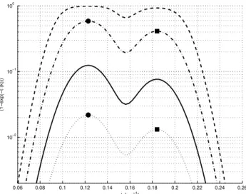
In Fig. 2, we present the complementary transmittance
(1−T )for the D1transition for different slant columns. For a Gaussian altitude profile with a FWHM of 20 km, a ref-erence value for the sodium vertical column is 5E9 cm−2 whereas the corresponding slant column is about 40 times larger (Fussen et al., 2004), i.e. 2E11 cm−2. For the weak absorption regime, the complementary transmittance is close to the optical thickness and therefore proportional to the os-cillator strength. When using the vertical column value we find a ratio D1a/D1bof 1.658, close to the expected value of 5/3 = 1.667 in the optically thin limit. For the corresponding slant column, we find a ratio of 1.424, suggesting a significa-tive deviation from the linear regime.
Integrating Eq. 3 in the frequency space over a1νinterval, we may define an effective transmittanceT¯ and the associ-ated effective cross sectionσ¯ as:
¯
T=exp(− ¯σ N )=U ν0 c1ν
Z
exp−τ0exp−x2dx (5) The equation above indicates that the effective cross section
¯
0.06 0.08 0.1 0.12 0.14 0.16 0.18 0.2 0.22 0.24 0.26 10−2
10−1 100
k [cm−1]
(1−exp(−
τ
(k)))
Fig. 2. Theoretical complementary transmittances for the D1aand
D1bsodium absorption lines as function of wavenumber difference
(the zero of the wavenumber range is 16 956 cm−1) for different
columns; dotted line: N= 5E9 cm−2; full line: N= 3E10 cm−2;
dashed-dotted line:N= 2E11 cm−2; dashed line:N= 1E12 cm−2;
dots and squares refer to the maxima of the the D1a and D1b
ab-sorptions for the sodium reference vertical and slant columns. In
the weak absorption regime, the ratio D1a/D1bshould be equal to
5/3.
In Fig. 3, the doublet absorption features of the experimen-tal transmittance were retrieved by fitting a double Gaussian shape
T (λ,h)=1−a1(h)exp
−(λ−(a3(h)+0.5984nm) a4(h)
)2
−a2(h)exp
−(λ−a3(h) a4(h)
)2
(6) with identical width for both lobes (0.5984 nm is the theoret-ical separation of the absorption doublet) and after having re-moved the baseline transmittance by using a low-order poly-nomial . This example is shown at a tangent altitude of 90 km for a latitudinal bin 70◦−80◦in which a large number of Sir-ius occultations with a high SNR ratio were available. The retrieved centroid of the D2line is 589.29 nm with a FWHM width of 0.46 nm a number that is close to the pre-launch value of 0.54 nm.
3 Results and validation
3.1 Observation of polar mesospheric clouds (PMC)
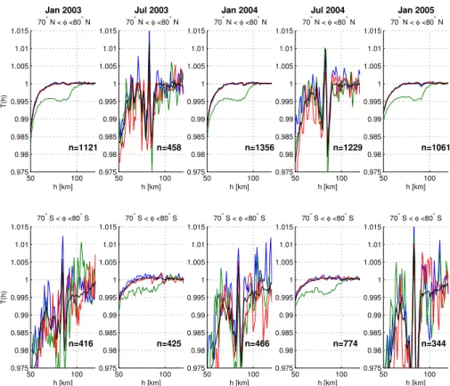
The sodium retrieval procedure described above has been applied to the full GOMOS data set. The intercompari-son of the binned transmittances for different seaintercompari-sons and observation modes (dark limb/bright limb) shows very dif-ferent situations. In Fig. 5, we focus on the polar regions
109 1010 1011 1012 0.2
0.3 0.4 0.5 0.6 0.7 0.8 0.9 1
N [cm−2]
ρ
V S
Fig. 3.Relative effective cross section as a function of sodium
col-umn for different temperatures; dotted line: T=100 K; full line:
T=200 K; dashed line: T =300 K. The arrows refer to the
refer-ence values for the vertical column (V) and slant column (S).
587 587.5 588 588.5 589 589.5 590 590.5 591 591.5 592 0.9955
0.996 0.9965 0.997 0.9975 0.998 0.9985 0.999 0.9995 1 1.0005
λ [nm]
T
Fig. 4.Diamonds: the median transmittance (of 1121 occultations)
measured between 70◦N and 80◦N during January 2003. Thin full
lines: individual D2and D1absorptions assuming to have the same
instrumental line spread function. Thick line: best fit for the total transmittance (with baseline removed).
50 100 0.975 0.98 0.985 0.99 0.995 1 1.005 1.01 1.015 h [km] T(h) Jan 2003
70° N < φ <80° N
n=1121 50 100 0.975 0.98 0.985 0.99 0.995 1 1.005 1.01 1.015 h [km] Jul 2003
70° N < φ <80° N
n=458 50 100 0.975 0.98 0.985 0.99 0.995 1 1.005 1.01 1.015 h [km] Jan 2004
70° N < φ <80° N
n=1356 50 100 0.975 0.98 0.985 0.99 0.995 1 1.005 1.01 1.015 h [km] Jul 2004
70° N < φ <80° N
n=1229 50 100 0.975 0.98 0.985 0.99 0.995 1 1.005 1.01 1.015 h [km] Jan 2005
70° N < φ <80° N
n=1061 50 100 0.975 0.98 0.985 0.99 0.995 1 1.005 1.01 1.015 h [km] T(h)
70° S < φ <80° S
n=416 50 100 0.975 0.98 0.985 0.99 0.995 1 1.005 1.01 1.015 h [km] 70° S < φ <80° S
n=425 50 100 0.975 0.98 0.985 0.99 0.995 1 1.005 1.01 1.015 h [km] 70° S < φ <80° S
n=466 50 100 0.975 0.98 0.985 0.99 0.995 1 1.005 1.01 1.015 h [km] 70° S < φ <80° S
n=774 50 100 0.975 0.98 0.985 0.99 0.995 1 1.005 1.01 1.015 h [km] 70° S < φ <80° S
n=344
Fig. 5. Median transmittances as a function of tangent height for polar bins during the months January and July from 2003 till 2005. The
number of occultations in the bin is indicated byn. In each subplot, red and blue colors correspond to control pixels (with only a smooth
ozone absorption) whereas the green color represents a pixel associated with the D2sodium absorption that exhibits a depression due to the
Na mesospheric layer. The black curve is the mean transmittance in a 20 nm window around the the Na absorption region. Close to summer solstices in each hemisphere, PMC dips and “flashes” are clearly seen around 83 km, for all wavelengths.
579.7–599 nm to filter out most of the residual noise. In the winter solstice cases, the sodium absorption is clearly visible whereas the control pixels and the mean window transmit-tance only show smooth and weak extinction due to ozone absorption in the Chappuis band and to Rayleigh scatter-ing. The summer solstices exhibit a remarkable and repro-ducible feature in both hemispheres: around 83 km, a sharp “emission” peak appears that affects all pixels of the spec-tral window. In view of the considered season and latitude, these peaks are attributed to the scattering of solar light by polar mesospheric clouds (PMC) into the GOMOS line-of-sight. Some supplementary scattering features are also visi-ble at lower altitudes although less reproducivisi-ble. It has been suggested by Plane et al. (2004), that the mesopheric metal-lic layers may act as nucleation seeds for the formation of PMC’s, showing a strong anticorrelation in their respective abundances. Na absorption is still visible in presence of PMCs but these are very narrow layers with limited spatial extent and there is no guarantee that GOMOS is observing Na and PMC’s in the same air mass. On the other hand, Gard-ner et al. (2005) showed that removal on PMCs is required to model the summertime Fe and Na layers over South Pole.
3.2 Inversion and retrieval of sodium concentration profiles
In the use of an optimal estimation method, the selected a priori information is crucial to avoid any bias in the retrieval. But so far, there does not exist a validated climatology of the global sodium distribution. Therefore we have preferred not to use an optimal estimation technique for retrieving the ver-tical profile of sodium concentration but instead to limit the number of retrieved parameters by imposing a generalized Gaussian distribution as:
n(z)=n0exp
− |z−αzp |ǫ
(7) wheren0is the peak concentration at altitudezp. The sodium
concentration peak extends over a region of typical sizeα
whereas the exponentǫexpresses the sharpness of the max-imum concentration. The forward model contains then only four parameters to retrieve (n0,zp,αandǫ) this small
0.996 0.997 0.998 0.999 1 50
60 70 80 90 100 110 120
T(h)
h [km]
GOMOS retrieval +100 K −100 K
1 1.2 1.4 1.6 1.8 2 50
60 70 80 90 100 110 120
D2/D1
h [km]
GOMOS retrieval +100 K −100 K
n
Na(z) [cm −3]
h [km]
0 1000 2000 3000 4000 5000 50
60 70 80 90 100 110 120
Fig. 6. Inversion of the measured effective transmittance profile for January 2003 in the latitudinal bin 70◦N–80◦N. Left side: effective transmittance versus tangent height; circles: measured values; green full line: best modeled value; red and blue lines: same conditions as for
green line but with +100 K (respectively−100 K) added to the used climatological temperature profile. Right side: top: D2/D1ratio for the
same case; bottom: retrieved Na vertical profile with its error bar envelope.
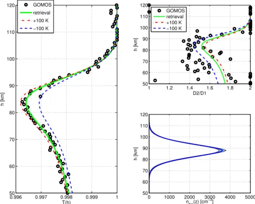
transmittance is built from the spatial integration of highly re-solved partial optical thicknesses along the optical path, fol-lowed by a spectral integration over the Maxwell-Boltzman distribution and finally reduced to an effective transmittance over the same wavelength interval on which equation 6 has been fitted. The inversion then proceeds through standard non-linear minimization techniques to retrieve (n0,zp,αand ǫ) and the associated error budget.
In Fig. 6, we present the result of the inversion for Jan-uary 2003 between 70◦N and 80◦N. In the left panel, the green curve is the best effective transmittance matching the observed values as a function of the tangent height. No-tice the typical asymmetric shape of the transmittance profile when the line-of-sight crosses a thin absorbing layer: a sharp edge at higher tangent heights (upper side of the layer) fol-lowed by a smoother dependence due to the Earth’s curvature as the tangent height decreases. In the same panel, we have also plotted the transmittances that would be caused by the same sodium concentration profile with a homogeneous tem-perature bias of±100 K added to the climatological values. Clearly, a precision of 10 to 20 K in effective temperature re-trieval would be difficult to achieve with respect to the avail-able SNR. In the right part of the figure, the top panel rep-resents the D2/D1ratio obtained for the same case whereas the bottom panel shows the retrieved sodium profile and the associated error bar envelope.
3.3 Validation
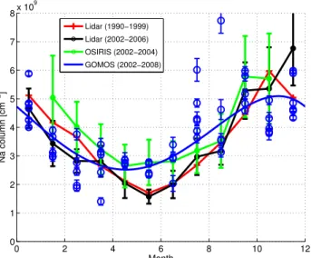
0 2 4 6 8 10 12 0
1 2 3 4 5 6 7 8x 10
9
Month
Na column [cm
−2]
Lidar (1990−1999) Lidar (2002−2006) OSIRIS (2002−2004) GOMOS (2002−2008)
Fig. 7. Intercomparison of Na column climatologies measured in
the 30◦–50◦ latitude band. Blue circles: GOMOS data (2002–
2008) and associated error bars; blue line: least-squares polynomial
fit for all GOMOS data; red line: Fort Collins (41◦N) lidar
cli-matology (1990–1999); black line: Fort Collins lidar clicli-matology (2002–2006) restricted to local time periods corresponding to GO-MOS observations; green line: OSIRIS measurements (2003–2004) from Gumbel et al. (2007).
We have also intercompared our data with recent re-mote sensing results of the mesospheric sodium layer by the OSIRIS instrument on board the ODIN satellite (Gumbel et al., 2007). We present the data extracted from Fig. 3 of the latter reference, for the period 2002–2004 and the agreement with GOMOS and Fort Collins looks reasonable. However, the validation of the OSIRIS data was performed with respect to the Fort Collins data whose climatology was also used to define the a priori profile and covariance matrix used in their optimal estimation method. This may cause a meaningless comparison when bad OSIRIS data (i.e. with large error bar measurements) could be forced to converge toward the refer-ence climatology.
In Fig. 8, we compare the time-altitude isopleths of GO-MOS Na data and the climatological Fort Collins data (1990– 1999). The same temporal evolution is observed with a somewhat weaker amplitude for GOMOS and an earlier min-imum. It should be kept in mind that the GOMOS data are interpolated at the Fort Collins latitude and that the natural observed variability is large. In the same figure, we have also plotted the annual mean of the GOMOS Na profile with its natural variability together with the mean Fort Collins data. Here again, we observe that the GOMOS peak value lies about 12% below the maximum of mean Fort Collins pro-file but within the associated retrieval uncertainty. This dif-ference is also compatible with the difdif-ference between both Fort Collins climatologies of 1990–1999 and 2002–2006.
Table 1. Parameters to be used for Eq. (8). A test value is
N (3.5,π4)=1.97E09 cm−2.
i fi a0 a1 a2 a3
1 1E09 0.1282 1.549 0.1780 0.03511
2 1 0.4017 0.8216 −0.1282 −0.2980
3 1E09 −0.2630 0.1121 0.6355 −0.3566
4 1 −1.5635 −3.0526 1.3802 1.7637
4 Climatology and interpretation
4.1 Na column
After a visual and systematic inspection of the retrieved Na concentration profiles for all bins, 66% of them can be con-sidered as having an acceptable or good quality (34% do not contain enough measurements or contain outliers or show a meaningless value with respect to their inversion error). To establish a mesospheric sodium climatology, the Na column
Nis a better estimator than the peak concentration value that might be partially anti-correlated with the peak width. We have modeled the full GOMOS data set as follows:
N (m,ϕ)[cm−2] =t0+t1cos
2π
12m+t2
+t3
ϕ+π
2 ϕ−
π
2
cos
2π
6 m+t4
ti≥1=fi
a0+a1ϕ+a2ϕ2+a3ϕ3
t0=3.28E09 (8)
wheremis the month andϕ is the geographic latitude ex-pressed in radians. The parameters of this bivariate fit are given in Table 1.
The fit uncertainty is aboutδN≃0.81E09 cm−2. In Fig. 9, we present the raw GOMOS data for the Na column and the bivariate fit. The most striking feature is the semi-annual oscillation at low latitudes merging into an annual cycle in the polar regions.
500
500
500
1000
1000
1000
1500
1500
2000
2000
1500
2500
2500 3000
2000
3500
2500
Decimal month
z [km]
0.5 1.5 2.5 3.5 4.5 5.5 6.5 7.5 8.5 9.510.511.5 80
85 90 95 100 105
500
500 500
1000
1000 1000
1500 1500 1500
1500 2000
2500
2000
3000
2500
3500
3000 4000
4500
Decimal month
z [km]
0.5 1.5 2.5 3.5 4.5 5.5 6.5 7.5 8.5 9.510.511.5 80
85 90 95 100 105
200
300
400 400
400
500
500
500
600
600 600
700
700
700 700
700
800
800
800 800
900 900
900
600
700
900
Decimal month
z [km]
0.5 1.5 2.5 3.5 4.5 5.5 6.5 7.5 8.5 9.510.511.5 80
85 90 95 100 105
Na concentration [cm−3]
z [km]
0 1000 2000 3000 80
85 90 95 100 105
Fig. 8.Top left: time-altitude Na concentration profiles (cm−3) measured by GOMOS in the 30◦–50◦latitude band. Top right: Fort Collins
Na climatology (1990–1991) at 41◦N. Bottom left: GOMOS measured uncertainty. Bottom right: blue: GOMOS annual mean in the
30◦–50◦latitude band with the associated uncertainty envelope; red: Fort Collins annual mean profile.
Fig. 10.Top: GOMOS sodium column climatology (as in Fig. 9). Bottom: raw GOMOS ozone partial column (between 80 and 100 km). Notice the similarities between the oscillation patterns.
4.2 Na peak altitude
The semi-annual oscillation pattern that is very pronounced in the equatorial regions is still visible at mid-latitude. In Fig. 11, we have intercompared the altitude of the Na layer obtained by GOMOS with those obtained in the 1990–1999 Fort Collins climatology. Clearly both data sets show the same behaviour. On average, the retrieved GOMOS peak altitudes do not differ from Fort Collins values by more than 1 km. The phase shift is not larger than 1 month, the GOMOS bin size. Also, there are periods of strong meridional gradient that nuance the accuracy of the comparison.
In Fig. 12, we present the complete climatology of the Na peak altitude. A general standard deviation of 1.6 km is observed. The importance of the mesospheric dynamics is again visible. Indeed, the zonal forcing by gravity wave breaking and the subsequent strong meridional circulation driven by the Coriolis force induces, through mass conser-vation, an important polar ascent at the summer pole and a subsidence at the winter pole (Smith, 2004). The ascent is al-most adiabatic and is the cause of the very cold mesospheric temperatures around summer solstice and the related pres-ence of PMC’s. The winter subsidpres-ence is also clearly visible on the Na peak altitude with a downward shift of about 4 km. Hereafter, we give an approximate fit for the dependence of
zpon the latitudeϕand decimal monthmthat only captures
the annual oscillation:
0 2 4 6 8 10 12
90.4 90.6 90.8 91 91.2 91.4 91.6 91.8 92 92.2 92.4
Decimal month
Peak altitude [km]
Fig. 11.Peak altitude of the Na layer. Red: Fort Collins climatology
(1990–1999); black dashed line: GOMOS data in the 30◦N–40◦N
bin; black dot-dashed line: GOMOS data in the 40◦N–50◦N
bin; blue: GOMOS weighted interpolation at Fort Collins latitude
(41◦N) and associated error bars.
zp(m,ϕ)[km] =(91.98−0.7723ϕ2)+(0.1364−0.6532ϕ2)
cos
2π
12m+1.302−0.887ϕ
−50 0 50 80
82 84 86 88 90 92 94 96 98 100
Latitude
Peak altitude [km]
89
89
89 89
89.5
89.5
89.5 89.5
90 90
90 90
90.5
90.5
90.5
90.5
90.5 91
91 91
91 91
91 91.5
91.5
91.5
91.5
91.5
91.5 91.5 91.5
92
92
92
92
92
92
92 92
92
92
92.5 92
92.5
93
Decimal month
Latitude [
°]
2 4 6 8 10
−80 −60 −40 −20 0 20 40 60 80
Fig. 12.Left panel: blue: retrieved peak heights (circles) in January and the approximate fit given by Eq. (9) (full line) showing the strong subsidence during polar winter; red: same data in July. Right panel: time-latitude isopleths for Na peak height.
4.3 Na peak concentration and width
Finally we present in Fig. 13 the maximum concentration of the mesospheric sodium layer as a function of time and lati-tude. A strong maximum is observed during winter in the po-lar regions of the northern hemisphere, with concentrations as high as 5000 sodium atoms per cubic centimeter. This maximum seems also present in the southern hemisphere but with some phase shift towards August.
When inspecting the scatter plot between retrieved peak concentrations and the full width half maximum of the Na profile, a partial anti-correlation was found. This is a di-rect consequence of sampling a narrow absorbing layer in limb viewing geometries. Most of the independent informa-tion is contained in the upper side of the layer and, when the tangent altitude decreases, the line-of-sight crosses the same layer under different angles and causes partial redundancy (see Fig. 6). In other words, it is difficult to distinguish be-tween situations of high peak concentration/narrow layer and low peak concentration/broad layer when the signal to noise ratio of the bin is not large enough. Integrating Eq. (7), one gets for the vertical column:
N=
∞
Z
0
n(z)dz≃n0
2αŴ1ǫ
ǫ =n0ζ (10)
whereζ can be interpreted as an effective width of the Na layer. But clearly,N is a more robust quantity geometrically related to the slant column and the measured transmittance. Therefore for the sake of robustness, we prefer to compute then0climatology as follows:
n0(m,ϕ)[cm−3] =
N (m,ϕ)[cm−2
]
ζ
ζ=(12.2e5±3.6e5)cm=(12.2±3.6)km
ǫ=2
α=√ζ
π =(6.9±2.0)km (11)
where an equivalent Gaussian profile is imposed, leading to an effective uncertainty onn0of about 38% (n0≃2690 atoms per cubic centimeter).
5 Conclusions
1000
1000 1000
1000
1000 1000
1000 1500
1500
1500 1500
1500
1500
1500 1500
1500
1500
1500
2000
2000 2000
2000
2000 2000
2000 2000
2000
2000
2500
2500
2500 2500 2500
2500
2500 2500
2000
2000
3000 3000
3000
3500 3500
4000 4000
2500
4500
2500
2500
3000 3000 3000
5000
1000
30003500 3500
2500
4000
4000
Decimal month
Latitude [
°]
1 2 3 4 5 6 7 8 9 10 11 −80
−60 −40 −20 0 20 40 60 80
Fig. 13.Peak concentration of mesospheric sodium [atoms/cm−3] as a function of time and latitude.
With respect to the preliminary results already published, we have demonstrated that Na slant columns produce par-tial saturation of the absorption lines whereas it is not the case for vertical columns, i.e. for lidar instruments. Roughly speaking, the full processing of these non-linear effects cause an enhancement of about 30% of our previous values for the Na column. We have demonstrated the potential effect of temperature on the retrieval even if we have limited the in-version to climatological values of temperature. However we would like to suggest a new method to measure meso-spheric temperatures with a good accuracy on a global scale. This could be achieved by a solar occultation experiment (possibly also with a limb scattering geometry but with a lower SNR) in which a low resolution spectrometer (about 0.1 nm) is measuring the sodium absorption doublet D2/D1 around 589 nm. Although the very narrow absorption lines are mainly broadened by the instrument line spread function and become small absorption features in the transmittance spectra, the measurement of the apparent optical thickness by differential absorption spectroscopy and of the D2/D1 ra-tio allows for the simultaneous retrieval of Na concentrara-tion and mesospheric temperature.
The principal result of this climatology is the discovery of a double pattern for the mesospheric sodium latitudinal and temporal distribution, i.e. a semi-annual equatorial os-cillation that merges into an annual polar osos-cillation. This was unreported so far in the literature and this pattern turns out to be quite similar to the ozone distribution measured by GOMOS. We have also shown the important subsidence observed during polar winter that demonstrates the accepted view of the general mesospheric circulation driven by the seasonal gravity wave break-up. Although comprehensive chemical models of the sodium mesospheric layer already exist, they only refer to the impact of temperature on the in-volved reaction rates for Na sources and sinks whereas this
paper demonstrates the necessity of using a realistic trans-port model capable of explaining the semi-annual equatorial oscillation. In particular, it has been suggested that the po-lar mesospheric clouds could be responsible for the strong decrease of the Na abundance during polar summer but this hypothesis still has to be validated against dynamical effects in the mesosphere. The strong sodium decrease in the polar summer mesosphere has been suggested to been a combina-tion of the effect of PMC and cold temperatures (Fan et al., 2007).
We have found a generally fair agreement in the validation of our results with lidar and limb viewing instruments. How-ever, we confirm that the sodium natural variability is high (30–50%) and this was already reported from ground-based climatologies. For this reason, we have approximated the Na vertical column with a robust fit capable of reproducing the annual and semi-annual phases and amplitudes. The winter subsidence of the Na peak was modelled in the same way. Finally, we described the sodium concentration and profile width from the total column fit by assuming an equivalent Gaussian profile for all bins.
In future work we will feed a general CTM model with our data. Also, we will investigate more accurately the shape of the Na concentration profile but only for the best available bins. We are also planning to cross validate the GOMOS transmittance data with Na airglow data that can possibly be retrieved from the upper and lower bands of the GOMOS sensor. Finally, we will process the full GOMOS data set in order to discover signatures of other mesospheric metallic layers.
Acknowledgements. This study was funded by the PRODEX 9
contract SECPEA under the authority of the Belgian Space Science Office (BELSPO).
Edited by: D. Murtagh
References
Arnold, K. S. and She, C. Y.: Metal fluorescence lidar (light detec-tion and ranging) and the middle atmosphere, Contemp. Phys., 44(1), 35–49, 2003,
Bertaux, J. L., Hauchecorne, A., Dalaudier, F., Cot, C., Kyr¨ol¨a, E., Fussen, D., Tamminen, J., Leppelmeier, G. W., Sofieva, V., Has-sinen, S., dAndon, O. F., Barrot, G., Mangin, A., Theodore, B., Guirlet, M., Korablev, O., Snoeij, P., Koopman, R., and Fraisse, R.: First results on GOMOS/Envisat, Adv. Space Res., 33, 1029-1035, 2004.
Chamberlain, J. W.: Physics of the Aurora and Airglow, Academic Press, New York and London, 1961.
Fan, Z. Y., Plane, J. M. C., Gumbel, J., Stegman, J., and Llewellyn, E. J.: Satellite measurements of the global mesospheric sodium layer, Atmos. Chem. Phys., 7, 4107–4115, doi:10.5194/acp-7-4107-2007, 2007.
Fricke, K. H. and von Zahn, U.: Mesopause temperatures derived
from probing the hyperfine structure of the D2resonance line of
Fussen, D., Vanhellemont, F., Bingen, C., Kyrola, E., Tamminen, J., Sofieva, V., Hassinen, S., Seppala, A., Verronen, P., Bertaux, J. L., Hauchecorne, A., Dalaudier, F., Renard, J. B., Fraisse, R., d’Andon, O. F., Barrot, G., Mangin, A., Theodore, B., Guirlet, M., Koopman, R., Snoeij, P., and Saavedra, L.: Global mea-surement of the mesospheric sodium layer by the star occul-tation instrument GOMOS, Geophys. Res. Lett., 31, L24110, doi:10.1029/2004GL021618, 2004.
Gardner, C. S., Plane, J. M. C., Pan, W., Vondrak, T., Murray, B. J., and Chu, X.: Seasonal variations of the Na and Fe layers at the South Pole and their implications for the chemistry and gen-eral circulation of the polar mesosphere, J. Geophys. Res., 110, D10302, doi:10310.11029/12004JD005670, 2005.
Gumbel, J., Fan, Z. Y., Waldemarsson, T., Stegman, J., Witt, G., Llewellyn, E. J., She, C. Y., and Plane, J. M. C.: Retrieval of global mesospheric sodium densities from the Odin satellite, Geophys. Res. Lett., 34, L04813, doi:10.1029/2006GL028687, 2007.
Kyr¨ol¨a, E., Tamminen, J., Sofieva, V., Bertaux, J. L., Hauchecorne, A., Dalaudier, F., Fussen, D., Vanhellemont, F., Fanton d’Andon, O., Barrot, G., Guirlet, M., Fehr, T., and Saavedra de Miguel,
L.: GOMOS O3, NO2, and NO3observations in 2002–2008,
Atmos. Chem. Phys., 10, 7723–7738, doi:10.5194/acp-10-7723-2010, 2010.
M´egie, G. and Blamont, J. E.: Laser sounding of atmospheric sodium interpretation in terms of global atmospheric parameters, Planet. Space Sci., 25, 1093–1109, 1977.
Plane, J. M. C.: Atmospheric chemistry of meteoric metals, Chem. Rev., 103, 4963–4984, 2003.
Plane, J. M. C., Murray, B. J., Chu, X., and Gardner, C. S.:Removal of Meteoric Iron on Polar Mesospheric Clouds, Science, 304, 426–428, doi:10.1126/science.1093236, 2004.
She, C. Y., Chen, S. S., Hu, Z. L., Sherman, J., Vance, J. D., Va-soli, V., White, M. A., Yu, J. R., and Krueger, D. A.: Eight-year climatology of nocturnal temperature and sodium density in the
mesopause region (80 to 105 km) over Fort Collins, CO (41◦N,
105◦W), Geophys. Res. Lett., 27, 3289–3292, 2000.
Smith, A. K.: Physics and chemistry of the mesopause region, J. Atmos. Sol.-Terr. Phy., 66, 839–857, 2004.


![Fig. 13. Peak concentration of mesospheric sodium [atoms/cm −3 ] as a function of time and latitude.](https://thumb-eu.123doks.com/thumbv2/123dok_br/16370988.191087/11.892.79.429.92.368/fig-peak-concentration-mesospheric-sodium-atoms-function-latitude.webp)
