An Energy Backpropagation Algorithm

Abstract— This paper presents an energy back-propagation algorithm (EBP). Learning and convergence processes of the standard backpropagation algorithm (SBP) are based on the energy function. The energy function is used with the convergence process to extract the nearest image for the unknown tested image. The EBP algorithm shows considerably better performance in terms of time of learning, time of convergence, and size of input image compared to the SBP algorithm.

Index Terms— Artificial neural networks, backpropagation algorithm, energy function, pattern recognition.

I. INTRODUCTION

Artificial neural networks have been successfully applied to problems in pattern classification, function approximation, optimization, pattern matching and associative memories [12]. One of the most popular neural networks is the layered feedforward neural network with a backpropagation (BP) least-mean-square learning algorithm [13]. Multilayer feed forward networks trained using the backpropagation learning algorithm [14]. The network edges connect the processing units called neurons. With each neuron input there is associated a weight, representing its relative importance in the set of the neuron's inputs. The inputs' values to each neuron are accumulated through the net function to yield the net value: the net value is a weighted linear combination of the neuron's inputs' values [15].

A backpropagation net can be used to solve problems in many areas [5]. But, the backpropagation algorithm has the limitation of slow convergence [17] and lengthy training cycles [8]. In order to overcome those drawbacks of the standard backpropagation (SBP) algorithm, the energy backpropagation (EBP) algorithm is proposed in this research.

The EBP algorithm adapts the following principles: (1) doing the learning and convergence processes for parts of the image and not all, (2) using small size of net will reduce size of learning weights matrices of the learning process, and (3) using the energy function based on Hopfield neural network will help converging to the correct image in high efficiency. Thus, the EBP algorithm will be efficient and accurate.

Manuscript received April 2, 2007.

Ahmad Hashim Hussein Aal-Yhia is with the Post-Graduate Institute for Accounting and Financial Studies, University of Baghdad, Baghdad, Iraq (corresponding author to provide phone: 00964-1-7780170; fax: 00964-1-7780306; e-mail: fingerprint192003@yahoo.com).

Dr. Ahmad Sharieh, is dean of King Abdullah II School for Information Technology, University of Jordan, Amman, Jordan (e-mail: sharieh@ju.edu.jo).

Fig. 1. Backpropagation neural network with one hidden layer [5].

A. Standard backpropagation algorithm

The feed forward backpropagation (FFBP) network is a very popular model in neural networks. It does not have feedback connections, but errors are backpropagated during training. Least mean squared error (LMST) is used. Many applications can be formulated for using (FFBP) network, and the methodology has been a model for most multilayer neural networks. Errors in the output determine measures of hidden layer output errors, which are used as a basis for adjustment of connection weights between the input and hidden layers. Adjusting the two sets of weights between the pairs of layers and recalculating the outputs is an iterative process that is carried on until the errors fall below a tolerance level. Learning rate parameters scale the adjustments to weights. A momentum parameter can also be used in scaling the adjustments from a previous iteration and adding to the adjustments in the current iteration [16].

B. Architecture

A multilayer neural network with one layer of hidden units (the Z units) is shown in Fig. 1. The output units (the Y units) and the hidden units also may have biases as shown in Fig. 1. The bias on a typical output unit Ykis denoted by wok; the Zjis

denoted voj. These bias terms act like weights on connections

from units whose output is always 1. Only the direction of information flow for the feedforward phase of operation is shown. During the backpropagation phase of learning, signals are sent in the reverse direction [5].

C. Training Algorithm

The backpropagation training algorithm is an iterative gradient algorithm designed to minimize the mean square error (MSE) between the actual output of a multilayer feedforward perceptron and the desired output. It requires continuous differentiable non-linearities. The following assumes a sigmoid logistic nonlinearity [10].

Step 1. Initialize weights and offsets

Set all weights and node offsets to small random

An Energy Backpropagation Algorithm

values.

Step 2. Present input and desired outputs

Present a continuous valued input vector x0, x1, . . . xN-1

and specify the desired outputs d0, d1, . . . d M-1. If the

net is used as a classifier then all desired outputs are typically set to zero except for that corresponding to the class the input is from. That desired output is 1.The input could be new on each trial or samples from a training set could be presented cyclically until weights stabilize.

Step 3. Calculate actual outputs

Use the sigmoid nonlinearity and formulas as in Fig. 2 to calculate outputs y0, y1 ... y m-1.

Step 4. Adapt weights

Use a recursive algorithm starting at the output nodes and working back to the first hidden layer. Adjust weight by

Wij(t+1) = wij(t) +

ηδ

jxi' (1)

In this equation, wij(t) is the weight from hidden node j

or from an input to node j at time t, xi' is either the

output of node j or is an input,

η

is a gain term, and

j

δ

is an error term for node j. If node j is an output node, then

j

δ

= yj (1 - yj) (dj - yj) , (2)

where dj is the desired output of node j and yj is the

actual output.

If node j is an internal hidden node, then

j

δ

= xj' (1 – xj')

∑

k

δ

k

w

jk , (3)

where k is over all nodes in the layers above node j. Interval node thresholds are adapted in a similar manner by assuming they are connection weights on links from auxiliary constant-valued inputs. Convergence is sometimes faster if a momentum term is added and weight changes are smoothed by Wij(t+1) = wij(t)+

ηδ

jxi' +

α

(wij(t)– wij (t - 1)) , (4)

where 0 <

α

< 1. Step 5. Repeat by going to step 2.

Fig. 2. Calculation of output for backpropagation training algorithm [9]

This paper is an extended of the research in [2]. In Section 2, the EBP algorithm will be introduced. In Section 3, the performance of the EBP algorithm will be compared to the

performance of the SBP algorithm. Section 4 concludes the work.

II. THE ENERGY BACKPROPAGATION ALGORITHM

A. The Energy Function

One system of updating is to update the units in sequence. The update mechanism posed by Hopfield (1982) chooses the unit randomly. Usually, all processing units must be updated many times before the network reaches a stable state. Each state of the network has an associated "energy" value, which is defined as:

v

v

t

j i

j ii j

ji

E

∑ ∑

≠

−

=

,

2

/

1

(5) When the network is in a stable state, the energy function is at a minimum, which may be local or global [9]. The existence of such function enables us to prove that the net will converge to stable set of activation, rather than oscillating. The function decreases as the system states change. Such a function needs to be found and watched as the network operation continues from one cycle to another. The least mean squared error is an example of such function. Energy function usage assures a stability of the system that cannot occur without convergence. It is convenient to have one value, that of the energy function specifying the system behavior [7].

The energy function is constant times the sum of products of outputs of different neurons and the connection weight between them, since pairs of neuron outputs are multiplied in each term [16]. The network with two neurons can be represented by four states: (00,01,10,11). The States of three-neuron network can be represented by a cube. In general, a network with n neurons has 2n states and can be represented by an n2-dimensional cube. When a new input is applied, the network moves from vertex to vertex until it stabilizes. If the input vector is partial or incomplete, the network stabilizes to the closest vertex. A number of binary vectors representing different patterns can be stored in the network. Here, in order to store input vectors, the energy equation is used to assign the weight values such that each memory vector corresponds to a stable state or the minimum energy equation of the network [9].

B. The EBP Algorithm

Fig. 3. Net of small size

The learning stage consists of learning algorithm. In this algorithm, we will divide the image into rows. Each row is divided into number of parts of two pixels, to be considered as a vector (V). This means there are four states for these vectors as shown in Fig. 4.

1 2 3 4

0 0 1 1

0 1 0 1

Fig. 4. The four states for the vectors.

Therefore, the learning process in the EBP algorithm for any image will result in four sets of learning weights matrices at maximum. Each set consist of two matrices: W1 and W2. The W1 represents the weights from input layer to hidden layer, and the W2 represents the weights from hidden layer to output layer. There are four sets of biases arrays at maximum. Each set consists of two arrays, which are called Wh and Wo. The Wh represents the biases of nodes of hidden layer, and Wo represents the biases of nodes of output layer. Each matrix of W1 and W2 will be of size 2x2, and each array of Wh and Wo will be of size 2x1.

Hence, each vector V, as shown in Fig. 4, will represent its own net. Each net has (W1 and W2, Wh and Wo). Therefore, we have only four nets as shown in Fig. 5.

Each vector V will be replaced by a number. This means we will replace all the parts (the vectors) in the image with numbers. These numbers represent the net.

Fig. 5. The four vectors with its own nets and numbers of nets.

The learning process of the proposed method for all vectors in the image will pass through two steps:

1. Testing whether the system has learned current vector before or not: The binary vector is examined. If it is saved with its learning weights matrices, then it is learned. Therefore, we will replace this vector by the number of its own net; otherwise, the vector is not learned.

2. Learning the vector: If the vector is not learned, it is entered to the backpropagation learning algorithm, then save its learning weights matrices, and save the number of net instead of vector.

The following steps present the learning algorithm: Step1: For x=1 to N {N: length of image} Step2: For y=1 to M step 2 {M: width of image} Step3:

IF binary vector is learned

Then Save the number of net for this vector and return to take the other vector.

Else enter the vector to the backpropagation learning algorithm, save learning weights matrices W1 & W2, and save number of net for this vector. C. The convergence stage

Fig. 6. Operation of identification the nearest image by energy function.

The identification process consists of the following steps: 1. Use the learning weights matrix W2 for current vector in

the unknown input image, with each W2 for the vectors in the images saved in the database, and extracts the Energy function (EV) between them. Thus, each image in the database will have value of its own Energy function. Therefore, extract the value of the first minimum energy function and the value of the second minimum Energy function. Then, extract the value of difference between them (Difference Next Close (DNC)).

2. Examine whether the system has learned the unknown input image before or not using the DNC value. If it is large value, then the unknown input image is learned. Therefore, the stored image with the minimum energy function, representing the nearest image for the unknown input image, is converged. However, if the DNC is small value, the unknown input image is not learned. Therefore, exit from the system. The DNC value depends on the image density and size.

The following algorithm presents the identification algorithm:

For x=1 to N {N: length of image} For y=1 to M {M: width of image} BEGIN

For all stored images do Begin

For all rows of stored images do

For the vector in the input image and learning weight matrix W2 do

Begin

EVk = -1/2 (

∑∑

= =

2

1 2

1

i j

W2ijk(input)* W2ijk (stored))

{Energy function for each vector} End;

E =

∑

=

VN

k 1

EVk {Energy function for each image}

End; END

DNC = E1 – E2 {E1: first minimum energy function, E2: second minimum energy function} IF DNC is large value

Then unknown input image is learned; therefore the stored image with the minimum Energy function (E) representing the nearest image for the unknown input image is converged.

IF DNC is small value

Then unknown input image is not learned, therefore exit from the system.

In the convergence algorithm, if unknown input image is learned, then converge the stored image with the minimum energy function (E). This is the nearest one for the unknown input image. In the same way of the learning algorithm, we divide the image into rows. Each row is divided into number of parts of two pixels size to be considered as a vector (V). Depending on the number of net and the backpropagation convergence algorithm, the vector (V) is converged. If the vector is converged by the backpropagation convergence algorithm before, it is converged using number of net.

The convergence algorithm is presented by following algorithm:

For x=1 to N {N: length of image} For y=1 to M step 2 {M: width of image}

For i=1 to NC {NC: the counter of the array (No Net) is contained n*m/2 of numbers of net saved instead of the vectors}

IF the current vector is not converged by the backpropagation convergence algorithm before, Then enter the current vector into the

backpropagation convergence algorithm and save the produced vector into the array of Converged Image (CI).

CI(x,y) = V(1,1) CI(x,y+1) = V(1,2)

Then, save the produced vector into the Converged Image (CI).

CI(x,y) = V(1,1) CI(x,y+1) = V(1,2) Endfor;

Endfor; Endfor.

III. EXPERIMENTS AND RESULTS

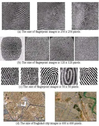
This section will be devoted to demonstrate the implementation of the EBP with experimental results and discussions. The experimental results are implemented on a Pentium IV, 2400 MHz using programs written in MATLAB. In our experiments, some samples of images are captured using database of fingerprint images [3, 11] and images of Baghdad city from space [6]. These images are of BMP and JPEG format. Fig. 7 shows some samples images, which are used in the experiments.

Fig. 7. Samples of fingerprint images and images of Baghdad city from space, which are used in the experiments.

The time of learning and converging processes of both the SBP and the EBP by using images with different sizes was measured. The net has only learned two images. The time averages of learning and converging processes were taken for five different readings. Table 1 shows the times of learning process when running the SBP and the EBP. Table 2 shows the times of convergence process of the SBP and the EBP. The SBP failed when the input array (input image) size was large. Therefore, we do not test images that have sizes 50x50, 128x128, 256x256 and 600x600 pixels on the SBP.

Table 1. The times of learning process on the SBP and the EBP algorithms.

Size of image (Pixel)

The average time of learning process in SBP

(Second)

The average time of learning process in EBP

(Second)

4x4 0.33 0.26

6x6 0.6 0.25

50x50 - 0.63

128x128 - 3.58

256x256 - 39.8

600x600 - 1118.4

The results show the process of learning process using the EBP algorithm is faster than the SBP algorithm. The results show that the converging process using the EBP algorithm is better than the SBP algorithm, when the image is larger.

Table 2. The times of converging processes in SBP and EBP algorithms.

Size of image

(Pixel)

SBP EBP

Time average of convergin

g process (Second)

Time average of identification

process (Second)

Time average of converging process (Second)

Time of entire converging

(Second) 4x4 0.006 0.009 0.015 0.024

6x6 0.006 0.006 0.024 0.03

50x50 - 0.62 0.07 0.69

128x128 - 4.57 0.47 5.04

256x256 - 19.1 2.07 21.17

600x600 - 85.93 11.62 97.55

IV. CONCLUSION

A backpropagation net can be used to solve problems in many areas. However, backpropagation algorithm has the drawback of slow convergence and lengthy training cycles. In order to overcome those drawbacks of the standard backpropagation (SBP) algorithm, the energy backpropagation (EBP) algorithm is proposed in this research.

The EBP algorithm deals with part of the image in performing the learning and convergence processes, uses small size of net to reduce the size of learning weights matrices of the learning process, and employees an energy function based on Hopfield neural network to speed converging to the correct image.

The energy function is computed from the sum of products of outputs of different neurons and the connection weight between them. The energy equation is used to assign the weight values such that each memory vector corresponds to a stable state or the minimum energy equation of the network.

Both the EBP and the SBP algorithms were implemented and tested on images of different sizes. The samples of the images were taken from a database of fingerprint images and images of Baghdad city. The images are of BMP and JPEG format. The time of learning and converging processes of both the SBP and the EBP algorithms were measured. The results indicate the superiority of the EBP algorithm over the SBP. However, the current results are encouraging for continuation of our work. We plan to make more experiments and practical implementations of the EBP algorithm.

REFERENCES

[1] R. Abdul Abbas, Fingerprint Classification Using Neural Network.

Unpublished master dissertation, University of Technology, Baghdad, Iraq, 1996.

[2] A. H. Aal-Yhia, TITLE of YOUR THESIS, Master Thesis, Computer Science Department, University of Jordan, Amman-Jordan, 2004. [3] Biometrix 8th WWW Fp-images. (2nd ed.) Retrieved August 10, 2003.

Available:

http://www.biometrix.at/fp-images.zip

[4] R. Duda and P. Hart, Pattern Classification and Scene Analysis. New York: Wiley, 1973.

[5] L. Fausett, Fundamentals of Neural Networks. (1st ed.), USA: Prenice-Hall, 1994.

[6] Image@2005 DigitalGlobe 8th HTTP sample.JPEG. (n. d.) Retrieved August 15, 2005. Available:

http://earth.google.com/

[7] W. Kinnebrock, Neural Network. Fundamentals, Applications, Examples.

USA: Prentice-Hill, Inc, 1995.

[8] B. Kosko, Neural Networks and Fuzzy Systems: A Dynamical Systems Approach to Machine Intelligence. USA: Prentice-Hall international, 1992.

[9] A. Kulkarni, Computer Vision and Fuzzy-Neural Systems. USA: Prentice Hall, 2001.

[10] R. Lippmann, “An introduction to computing with neural nets,” in IEEE. April 1987, 4-22.

[11] Neurotchnologija 3th WWW Fingercell_Sample_DB. (n. d.) Retrieved May 25, 2004.Available:

www.neurotchnologija.com/download/fingercell_sample_DB.zip.

[12] R. Parekh, J. Yang, and V. Honavar, “Constructive neural-network learning algorithms for pattern classification,” IEEE Transactions on Neural Networks. March 2000, Vol. 11, No.2.

[13] R. Rojas, “Neural networks, a systematic introduction,” in Springer. Berlin, 1996.

[14] D. Rumelhart, G. Hinton, and R.Williams, “Learning internal representations by error propagation,” in Parallel Distributed Processing: Explorations into the Microstructure of Cognition. Cambridge, MA: MIT Press, 1986, vol. 1.

[15] S. Stoeva, A. Nikov, “A fuzzy backpropagation algorithm,” Fuzzy Sets and Systems. 2000, 112, pp. 27–39.

[16] B. Vallurn, and V. Hayoriva, C++ Neural Network and Fuzzy Logic. (2nd ed.), USA: M&T publishing, 1996.