FUNDAC
¸ ˜
AO GET ´
ULIO VARGAS
ESCOLA DE ECONOMIA DE S ˜
AO PAULO
ANDR´
E SANDER DINIZ
Financial disruption as a cost of
sovereign default
FUNDAC
¸ ˜
AO GET ´
ULIO VARGAS
ESCOLA DE ECONOMIA DE S ˜
AO PAULO
ANDR´
E SANDER DINIZ
Financial disruption as a cost of
sovereign default
Disserta¸c˜ao apresentada `a Escola de Economia de S˜ao Paulo da Funda¸c˜ao Get´ulio Vargas, como requisito para a obten¸c˜ao do t´ıtulo de Mestre em Economia
´
Area do conhecimento: Macroeconomia
Orientador: Bernardo de Vasconcellos Guimar˜aes
Andr´e Sander Diniz
Financial disruption as a cost of sovereign
default
Disserta¸c˜ao apresentada `a Escola de Economia de S˜ao Paulo da Funda¸c˜ao Get´ulio Vargas, como requisito para a obten¸c˜ao do t´ıtulo de Mestre em Economia
´
Area do conhecimento: Macroeconomia
Orientador: Bernardo de Vasconcellos Guimar˜aes
Data de aprova¸c˜ao:
24/01/2014
Banca Examinadora:
Prof. Ph.D. Bernardo Guimar˜aes (Orientador)
EESP/FGV
Prof. Dr. Vladimir Kuhl Teles EESP/FGV
Agradecimentos
Ao Bernardo, por toda a dedica¸c˜ao e ajuda como professor e orientador. Pelo incentivo no dia-a-dia da elabora¸c˜ao deste trabalho e pelo est´ımulo nos caminhos da pesquisa em economia.
Aos meus pais Marco Tulio e Maria de F´atima, pela confian¸ca nas minhas escolhas, por terem me ensinado como ´e gratificante entender o mundo atrav´es dos estudos, pelo exemplo de realiza¸c˜ao na profiss˜ao e por estarem sempre presentes com conselhos e carinho, mesmo que a distˆancia tenha se tornado maior. `As minhas irm˜as Fl´avia e Juliana, por continuarem a ser as melhores companheiras de conversas, viagens e bobagens e, embora eu relute em aceitar que elas cresceram, por terem adquirido papel importante nas decis˜oes s´erias da vida.
`
A Izabela, pelo amor e cumplicidade, por estar sempre ao meu lado e ter tornado muito mais prazerosas as mudan¸cas dos ´ultimos anos, pelo amadurecimento que tivemos juntos e pelos planos que ainda vir˜ao.
Aos familiares e amigos de BH, em especial aos meus av´os, pelo apoio e interesse mesmo de longe e por representarem sempre a mineiridade que me faz sentir saudade de casa.
Ao Lehrer, por ter sido um grande irm˜ao na Galo-Perdizes, pelas doses semanais de cerveja, conversas, filmes e futebol e por sempre tentar me mostrar a importˆancia dos conflitos e de pensar fora da caixa. `A Bela, pela amizade desde a faculdade e por sua parcela de responsabilidade na minha decis˜ao acertada pela EESP.
Aos amigos da GV que, pela companhia em dias infind´aveis na biblioteca e outros muito melhores e bem longe dela, fizeram o mestrado mais leve e divertido. Ao Marcel, pela paciˆencia com minhas d´uvidas sobre o Dynare.
Aos professores Carlos Eduardo Gon¸calves, Luiz Ara´ujo e Vladimir Teles, pelos co-ment´arios e sugest˜oes na qualifica¸c˜ao e na defesa, que contribu´ıram bastante para a dis-cuss˜ao apresentada neste trabalho.
Aos professores Laura Carvalho e Clemens Nunes, pelas oportunidades de pesquisa e monitoria na EESP, que enriqueceram muito meu aprendizado durante o mestrado.
`
Abstract
This dissertation analyses quantitatively the costs of sovereign default for the economy, in a model where banks with long positions in government debt play a central role in the financial intermediation for private sector’s investments and face financial frictions that limit their leverage ability. Calibration tries to resemble some features of the Eurozone, where discussions about bailout schemes and default risk have been central issues. Results show that the model captures one important cost of default pointed out by empirical and theoretical literature on debt crises, namely the fall in investment that follows haircut episodes, what can be explained by a worsening in banks’ balance sheet conditions that limits credit for the private sec-tor and raises their funding costs. The cost in terms of output decrease is though not significant enough to justify the existence of debt markets and the government incentives for debt repayment. Assuming that the government is able to alleviate its constrained budget by imposing a restructuring on debt repayment profile that allows it to cut taxes, our model generates an important difference for output path comparing lump-sum taxes and distortionary. For our calibration, quantitative re-sults show that in terms of output and utility, it is possible that the effect on the labour supply response generated by tax cuts dominates investment drop caused by credit crunch on financial markets. We however abstract from default costs asso-ciated to the breaking of existing contracts, external sanctions and risk spillovers between countries, that might also be relevant in addition to financial disruption effects. Besides, there exist considerable trade-offs for short and long run path of economic variables related to government and banks’ behaviour.
Resumo
Este trabalho analisa de forma quantitativa os custos para a economia de um default soberano, num modelo onde bancos comprados em d´ıvida tˆem um papel cen-tral na intermedia¸c˜ao financeira para os investimentos do setor privado e enfrentam fric¸c˜oes financeiras que limitam sua alavancagem. A calibra¸c˜ao busca refletir econo-mias da Eurozona, onde discuss˜oes sobre risco de calote das d´ıvidas e programas de resgate aos governos tem sido temas centrais. Os resultados mostram que o modelo captura um importante custo apontado pela literatura emp´ırica e te´orica, qual seja, a contra¸c˜ao do investimento que segue um epis´odio de default, o que pode ser explicado pela piora no balan¸co do setor financeiro, limitando cr´edito e liquidez para o setor privado e aumentando os custos para o seu financiamento. O custo em termos de perda de produto, no entanto, n˜ao ´e suficiente para explicar a existˆencia de mercados de d´ıvida e os incentivos dos governos em honrar seus compromissos. Assumindo que a reestrutura¸c˜ao do perfil de pagamentos da d´ıvida imposta num caso de default permite ao governo aliviar sua restri¸c˜ao or¸cament´aria e cortar im-postos, o modelo apresenta resultados bastante distintos para impostos lump-sum e distorsivos. Para nossa calibra¸c˜ao, a resposta quantitativa de produto e utilidade mostra que ´e poss´ıvel que o efeito na oferta de trabalho gerado por cortes de impos-tos distorsivos domine a queda no investimento, causada pela escassez de cr´edito nos mercados privados. S˜ao abstra´ıdos, no entanto, os custos de default associados a quebras de contratos, san¸c˜oes externas e transbordamentos de risco entre pa´ıses, que podem ser bastante relevantes em adi¸c˜ao ao impacto sobre o cr´edito no sistema financeiro. Al´em disso, existem trade-offs consider´aveis na trajet´oria de curto e longo prazo das vari´aveis econˆomicas relacionados ao comportamento dos governos e dos bancos.
Contents
1 Introduction 1
2 Literature Review 5
3 Model 10
4 Calibration and Solution 21
5 Results 24
6 Final Remarks 33
References 35
A Banks allocation problem 37
B Other results 39
1
Introduction
Several contributions to the literature about debt crises have agreed that large output losses related to default episodes are necessary to explain why sovereign debt exists and is repaid (Panizza, Sturzenegger & Zettelmeyer, 2009). Furthermore, recent authors have identified theoretically and empirically that these output losses are associated to invest-ment drops, as a consequence of liquidity scarcity related to deteriorating banks’ balance sheet conditions following a default episode, since banks are an important creditor for government debt (Brutti, 2011; Borensztein & Panizza, 2008). The financial intermedi-ary channel is still a field to be explored by the literature when analysing the effects of sovereign risk/default for business cycles, when both goods producers and government depend on banks for credit purposes. There are two pronounced trade-offs emerging from this context: the first one is related to banks’ portfolio allocation, once they are able, up to some extent, to shift demand from government debt to firms loans and vice versa, in case one of their assets loses value. The second trade-off happens at the government level. It is reasonable to assume that a haircut alleviates government budget strain, opening some space for tax cuts and/or anti-cyclical spending, although debt ceiling and access to credit markets tend to be reduced following a default or a restructuring episode.
In this context, the aim of this dissertation is to explore the interaction between debt restructuring episodes - or haircuts - and the financial intermediary channel, allowing leverage-constrained banks to hold government and capital firms’s securities on the assets side. We build on Gertler & Karadi (2011) and Gertler, Kyiotaki & Queralto (2012) introducing a public sector that issues debt and taxes households to finance its spendings. Banks are the only agent that can buy this sovereign securities (we do not allow households to buy debt directly, to induce financial frictions in this market). We simulate a debt restructuring episode in which banks suffer portfolio losses but households might pay less taxes, because debt level is reduced in the short run. Through the financial accelerator approach we explore the consequences of such a framework.
The recent crisis of the highly indebted Euroarea economies has contrasted govern-ment efforts for fiscal tightening, a necessary condition for obtaining external bailout, and financially constrained workers with eroded earnings by higher taxation. Hence we compare, on the government side, the effects of lump-sum versus distortionary taxation for agents decisions and the response of the economy following debt restructuring. We depart from most part of the literature by modeling a closed economy, what we justify as an intention to represent the Euroarea as one big (closed) economy whose government has a high debt-to-GDP ratio and banks have a long position on debt claims.
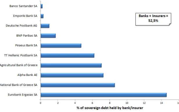
(2012) points out that one important consequence of the subprime financial crisis was a re-versal in investor base for government securities for some advanced G20 economies. Prior to the crisis, global financial integration encouraged the growth of non-resident holders of sovereign debt and credit booms reduced the proportion of government debt to total domestic financial assets for most domestic investors. This trend has stopped and in many cases reversed after the start of the crisis, in order to cope with deleverage of financial institutions and larger issuance of government securities caused by high deficits. Particu-larly in Europe, the application of the Basel Accords through the Capital Requirements Directive motivates banks to hold large amounts of government debt on their portfolios. According to European law, government bonds issued in domestic currency have a 0% risk weight for regulatory purposes. This special treatment for sovereign bonds issued in Euros creates a tendency for European banks to hold a significant worth of government debt on their balance sheets.
Figure 1: Greek government debt: top creditors from financial institutions, August 2013
Source: Bloomberg
With the recognition that banks are actually more important holders of government debt than foreign investors, consequences for the banking sector have been increasingly considered as an important cost of default for the domestic economy, and default episodes tend to magnify the probability of a banking crisis (Borensztein & Panizza, 2008).
Having important holdings of sovereign debt among its assets, banks might have be-come more vulnerable to sovereign risk, that tends to spillover to private credit markets. Figure 2 shows evidence of sovereign-bank contagion, observed by the increase in corre-lation between CDS spreads from sovereign debt and non-financial corporate debt in the last years, mainly for Euroarea countries most affected by debt crises.
Figure 2: CDS spreads from sovereign and non-financial corporate debt
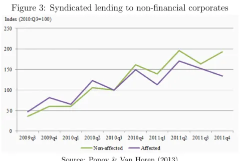
Evidence also exists that lending by banks that where above the median in terms of GIIPS debt holdings has decreased, as the debt crises became more apparent. Figure 3 presents evolution of syndicated lending by banks holding GIIPS debt, above the median of the sample (affected) and below the median (non-affected). One can see that there was an inversion in credit provision from these institutions in the aftermath of the debt crises.
Figure 3: Syndicated lending to non-financial corporates
Source: Popov & Van Horen (2013)
By modelling a closed economy where banks play a central role for liquidity provision and government debt is one important asset, we try to capture these observations from european data quantitatively, addressing costs of default in terms of private investment, output and utility. Moreover we investigate effects of different taxation schemes for agents’ response to the shock in government finance.
2
Literature Review
Our work intends to contribute quantitatively to the literature on sovereign debt crises and default episodes, assuming a closed economy where domestic banks are the only gov-ernment creditor and hence investigating the financial accelerator channel in the presence of sovereign risk. So we start this section with a brief overview of prominent contribu-tions to the literature of financial friccontribu-tions, on which our model is built. Then we present some important research findings about debt crises and default episodes and relate the current theoretical and empirical debates - motivated largely by recent developments of the european crisis - to our contribution.
2.1
Financial Frictions and Business Cycles
The literature about the role of financial frictions to business cycles had initially aimed at incorporating various empirical evidences of credit market frictions into the traditional Real Business Cycle and New Keynesian frameworks, that abstracted from these features and regarded financial markets and firms’ balance sheets as not being able to affect real economy. Introducing financial frictions by means of an agency problem, Bernanke & Gertler (1989), Carlstrom & Fuerst (1997) and Bernanke, Gertler & Gilchrist (1999) show that endogenous dynamics in credit markets are able to magnify the effects of external shocks in the economy. This channel is known as the ”financial accelerator”.
In all these three frameworks, production is driven by entrepeneurs and financed by both their own equity and by external finance. There is an assimetric information problem, in which only entrepeneurs observe the returns from their investment projects. Thus there is a costly state verification problem, once returns from entrepeneurial projects are not directly observable by lenders, who must pay a fee to observe realized returns. In this setup, borrowers’ balance sheet conditions will influence the costs for external financing. The financial accelerator arises because an external productivity shock that reduces entrepeneurs’ net worth can raise external financing costs, reducing demand for new investments and lowering economic activity. The initial economic slowdown provoked by the shock is amplified as a consequence of the financial frictions that limit credit supply and raise costs for productive investment.
For Kiyotaki & Moore (1997), the main source of variation in borrowers’ net worth are endogenous fluctuations in asset prices that serve as collateral for obtaining loans. In their model, borrowers credit limits depend on the value of collateralized assets. If a shock lowers the value of the collateralized assets, then firms must cut back their investment projects, which affects their cash flows and net worth, and spreads the effects of the initial shock.
Karadi (2011) and Gertler, Kiyotaki & Queralto (2012) also build a financial accelerator model in which banks play a central role. Firms that produce output have to issue securities in order to obtain funds for capital acquisition. Banks buy these securities using deposits from households. The credit friction is however motivated in a different way: firms face no direct frictions to obtain funds for investment, but banks do face constraints to obtain deposits from households. This happens because banks have incentives to deviate funds to their owners in form of dividends. To avoid this, depositors place a moral hazard constraint that limits banks’ ability to raise funds and creates frictions in credit markets. Like in the other models, these frictions can work to amplify the effects of exogenous shocks to business cycles.
In a recent research, Boissay, Collard & Smets (2013) expand the financial acceler-ator framework, being able to generate credit freezes and banking crises as a result of endogenous pro-cyclical movements in banks’ balance sheets. Their results are different from Bernanke, Gertler & Gilchrist (1999) and Gertler & Karadi (2011) in the sense that exogenous shocks are secondary to generate crises. In their model, crises can be generated as a development of endogenous financial imbalances, such as credit booms.
2.2
Debt crises, sovereign risk and default costs
The economic theory of sovereign debt is concerned with the investigation of the reasons why sovereign debt markets exist, debt crises and defaults occur and the incentives and costs for creditors and debtors surrounding these episodes. In a recent survey of the literature related to sovereign debt crises, Panizza, Zettelmeyer & Sturzenegger (2009) conclude that external penalties are not the main reason why governments repay their debts - as many of the first contributions suggested1, since there is little evidence of
significant creditor enforcement capacity, longstanding exclusion from financial markets and/or important trade sanctions. Hence there should exist important internal costs following defaults, in terms of output losses for the debtor country, that explain the sustainability of high levels of sovereign debt and the efforts made to honour it2. Recent
empirical and theoretical literature on debt crises has thus aimed at exploring the channels through which default can trigger domestic output costs.
1
Eaton & Gersovitz (1981) show that, under certain conditions, permanent exclusion from financial markets, even in the absence of creditors enforcement ability, can explain the existence of sovereign debt markets and guarantee debt repayment. Bullow & Rogoff (1989) avoid the hypothesis that the threat of future exclusion from credit markets guarantees debt repayment. They explain the existence of lendings to sovereigns by the possibility of direct sanctions such as trade constraints or country’s assets capture in case of default.
2
Following this line, Brutti (2011) investigates the connection between sovereign risk and liquidity crises without the need for foreign creditors existence or exclusion from credit markets. Supposing government bonds are a necessary source of liquidity for the economy and that government is not able to differentiate between foreign and domestic creditors, he shows that debt repayment tends to be procyclical and represents a wealth transfer from workers to entrepeneurs.
Some recent papers have proceeded in this connection between sovereign risk and the financial sector. The idea that sovereign risk influences banks financing conditions has been widely explored by empirical literature. Contagion between governments and financial sector can be based on the concept of ”sovereign ceilling”, a policy from credit rating agencies that states that no corporate debt can be riskier that the firm’s country government debt. If this rule holds, riskier government debt will imply directly a higher risk for banks assets and securities, and a rise in spreads required by banks creditors. The rise in financing costs can lead to cuts in credit supply by banks.
Bank of International Settlements (2011) reports the changes in bank’s balance sheets and funding conditions as a consequence of the mentioned european debt crisis and refers to four main channels through which sovereign risk may affect banks’ funding costs and risk. First, an increase in sovereign risk may affect the market value of banks’ bal-ance sheets directly through its holdings of sovereign debt, as bonds are subject to value losses. Second, sovereign bonds are largely used as collateral to wholesale funding. Third, sovereign ratings’ downgrades can often lead to downgrades of banks’ debt ratings. Fourth, the weakening of fiscal positions may reduce the value of explicit and implicit guarantees given by governments to banks. All this four channels might affect somehow the risk of banks’ activity, raising their costs to obtain resources and consequently the supply of credit for the economy.
Trying to access contagion between sovereign risk and systemic risk in the financial sector, De Bruyckere et al (2013) use the spreads over credit default swaps (CDS) as a measure of credit risk, controlling for fundamentals and common market risk parame-ters. They find evidence in favor of sovereign-bank contagion (excess correlation between sovereign and banks CDS spreads) in European economies between 2006 and 2011. Con-tagion was greater within countries, but foreign conCon-tagion was also significant. Besides, contagion was higher for more exposed banks, i.e., those ones that hold greater amounts of sovereign bonds on their balance sheets (above the median of the sample).
The empirical evidence found in data that emerged in the aftermath of the global financial crisis and particularly during the debt crises episodes in the Eurozone has mo-tivated theoretical and quantitative model-based investigations of the links connecting sovereign risk and macroeconomic stability, mainly during fiscal consolidation discussions, zero lower bound episodes and bailout schemes.
Corsetti et al (2012) and Corsetti el al (2013) develop macro-models with financial frictions using Curdia & Woodford’s (2008) framework. In their model financial inter-mediation appears because in equilibrium there are two types of agents, borrowers and lenders. Frictions in banking activity appear because there are costs associated to inter-mediation, since it consumes real resources and can be subject to frauds. This frictions limit the resources available for lending and induce a spread between deposits and loan rates. The authors assume this spread is exogenously connected to sovereign risk and depends on the expected debt level. Simulations find that sovereign risk can raise risk premia that financial intermediaries face and exacerbate effects of cyclical shocks. The latter also analyse the sovereign risk channel and the international transmission of risk in a model of the Euroarea, but foccusing on the coordination of fiscal policy between ”core” and ”periphery” countries and on the effects of recent ECB measures as a way to reduce sovereign risk and spreads in the indebted countries.
Bolton & Jeanne (2011) analyse theoretically the consequences of debt crises in a financially integrated world, where the government debt of a country can be used as col-lateral by banks from other countries, in order to diversify risk. However, the presence of sovereign risk in one country can be easily spread to the others, as banks have di-versified portfolios of foreign debt, giving rise to systemic risk, such as observed in the european episode. In this case, the adverse consequences for costs and availability of bank credit quickly reach other economies whose banks hold some amount of foreign debt, with implications for the real economy through the channels above mentioned.
Guerrieri, Iacoviello & Minetti (2012) analyse the international trasmission of sovereign risk and default in the Eurozone by means of bank’s balance sheet channel. Default is triggered by large negative productivity shocks. There are two conflicting effects: a portfolio substitution one, when banks migrate to capital assets instead of debt and a balance sheet effect, because debt in portfolio loses value. The authors find dominance of the second effect, with default triggering a contraction in credit supply, due to the presence of leverage constraints. Default in the so called ”periphery countries” spillsover to banks in the core, also leading to lower investment and output.
investment costs, this way of modeling can be more suitable for quantitative simulation that seeks to resemble moments from observed data.
3
Model
The model builds on Gertler & Karadi (2011) and Gertler, Kiyotaki & Queralto (2012). The framework is a stochastic general equilibrium model in which all variables are ex-pressed in real terms (RBC like), abstracting from price and wage rigidities and monetary policy.
Differently from most part of the literature related to sovereign default, our model deals with a closed economy whose banks have long positions on government debt, that amount to a large fraction of GDP. One could think our economy as representing the whole Euroarea, where the larger fraction of sovereign debt of each country is held either by domestic creditors or by financial institutions within the block.
The economy is populated by five types of agents: households, goods producers, capital producers, bankers and government. If we do not consider government, the model becomes a Financial Accelerator one, a simplified version from Gertler & Karadi (2011). In this set up, including a government that issues non-state contingent debt held only by banks and assuming default possibility, we induce an asset allocation problem for banks and new dynamics to the business cycle in response to shocks to debt prices or haircuts on bonds’ face value.
3.1
Households
There is a representative household with a continuum of members of measure unity, with a fraction 1-f that are ”workers” and a fraction f that are ”bankers”. Workers supply labour and return wages to the family, while bankers own a financial intermediary and return dividends to their household. Households can save in form of deposits held by intermediaries. They supply funds to banks in form of non-contingent short term debt (deposits, denoted Dt), that pay a risk-free gross real return rate Rt. Although each
household effectively owns a bank, its deposits are spread among all banks in the economy, including the ones they do not own. We additionally assume households’ direct purchase of bonds is very costly and hence they are not able to buy government bonds directly.
Hence households choose consumption, labour supply and riskless debt to maximize expected discounted utility. We assume preferences in logaritmic form that follow GHH specification, in order to avoid wealth effects on labour supply (Greenwood, Hercowitz & Huffman, 1988).
Et
∞
X
i=0
βilog
Ct+i−
ψ 1 +ϕL
1+ϕ t+i
(1)
Households are subject to the following budget constraint:
Where Wt is the wage rate, Tt are lump sum taxes payed to the government and
Πt are the dividends distributed from the ownership of nonfinancial firms and banks.
Later we impose distortionary taxes on labour supply to compare the effects of shocks on government budget constraint with the case of lump-sum taxes.
From the first order conditions for labour supply and consumption/saving, we get:
Wt=ψLϕt (3)
EtβΛt,t+1Rt+1 = 1 (4)
with
̺t≡
Ct−
ψ 1 +ϕL
1+ϕ t+i
−1
Λt,t+1 ≡
̺t+1
̺t
and where̺tis marginal utility of consumption and Λt,t+1 is the households’ stochastic
discount factor.
The environment includes an i.i.d. probability (1−θ) that a banker exits from period to period. In order to maintain the fraction in each occupation constant over time, at each period we assume that a fraction (1−θ)f workers randomly become bankers. Workers that become bankers receive a ”start up” capital from the household to start business. Expected survival time of a bank is thus1/(1−θ). This finite life of a banker is a mechanism
to prevent bankers from accumulating wealth so as to overcome its financial constraint, which will be presented soon.
Households also own nonfinancial firms (capital and goods producers). They are though not able to acquire capital directly nor to provide funds to these firms. All financial intermediation for production must be made by means of a bank.
3.2
Goods producers
The representative goods producer firm produces output in a competitive market, using labour and capital in a Cobb-Douglas constant returns to scale technology:
Yt =KtαL1
−α
t (5)
with 0< α <1.
As usual, firms choose labour to satisfy the condition that real wage rate equals marginal product of labour:
Wt = (1−α)
Yt
Lt
In order to produce in the following periodt+1, firms need to buy the amount of capital Kt+1at the end of periodtfrom capital goods producers. To finance this acquisition, firms
issue securitiesStso that the value of the issued securities equals by arbitrage the value of
the capital to be bought. The intermediaries buy this securities and give funds to goods producers. Denoting Qt as the price of one unity of capital, we have:
QtKt+1 =QtSt
There are no frictions in this process. Intermediaries have perfect information about the firm and about future payoffs, so securities are state-contingent. Frictions exist within the process of banks obtaining resources from households. This frictions affect the amount of funds supplied to firms and hence can affect the required rate of return for firms to pay. The price of one unity of capital will be determined endogenously in the capital producers problem, to be showed next.
In order to satisfy the zero profit condition in the competitive market, goods producers buy capital goods up to the point that gross profits per unit of capital, Zt, equal the
marginal product of this input.
Zt=
Yt−WtLt
Kt
=αYt Kt
(7)
A firm that sells St securities to acquire capital must return all its profits in the next
period to the bank. Call Rkt the gross return to capital in time t, the amount a bank
obtains as a return over each unity of credit supplied in the form of acquired securities. The representative goods producer owes a bank an amount QtStRkt+1 at the end of the
period. This value equals the sum of the profits, Πf t, obtained through capital utilization
in production (gross of capital remuneration) and the market value of the effective non-depreciated capital, that could be sold back in the market at the end of production.
QtStRkt+1 = Πf t+1+ (1−δ)Qt+1Kt+1
Substituting for Πf t and St:
QtKt+1Rkt+1 =Yt+1−Wt+1Lt+1+ (1−δ)Qt+1Kt+1
Dividing both sides byKt+1:
QtRkt+1 =α
Yt+1
Kt+1
+ (1−δ)Qt+1
Rkt+1 =
Zt+1+ (1−δ)Qt+1
Qt
(8)
3.3
Capital producers
At the end of each period, capital producers build new capital for next period using input of final output and then sell back to goods producers at price Qt. They are subject
to convex adjustment costs in this process. Adjustment costs are maintained because the provide quantitative performance and add little complexity to the model (Gertler & Kiyotaki, 2010). They prevent a very quick response of investment to economic flutuations and help generate some empirical observed effects in labour, consumption and product responses.
Capital production occurs in a competitive market. As firms are onwed by house-holds, the objective of a capital producer is to choose investment It in order to maximize
discounted profits, taking price of capitalQt as given.
Adjustment costs will be a convex function of investment flow. Capital producers’ problem is given by:
maxEt
∞
X
τ=t
βτ−tΛ t,τ
QτIτ−
1 +f
Iτ
Iτ−1
Iτ
(9)
withf(1) =f′
(1) = 0 andf′′
(1)>0. Outside steady state is possible to have non-zero profits, that are transfered to the household.
First order condition for investment is given by:
Qt= 1 +f
It
It−1
+ It
It−1
f′
It
It−1
−EtβΛt,t+1
It+1
It
2 f′
It+1
It
(10)
This condition states that capital price will equal marginal cost of investment. The adjustment cost function will assume the form:
f(.) = ηi 2
It
It−1
−1 2
whereηi is a parameter that refers to the inverse elasticity of investment with respect
to capital price.
3.4
Government
Government spending is exogenous. We assume in government consumes always a given amount ¯G:
Gt = ¯G (11)
Lump sum taxes are set in order to prevent large deviations of debt level from steady state:
Tt= ¯T +γ(Bt−B)¯ (12)
whereBt is the level of bonds (debt) in the market at timet and in steady state,Bt= ¯B.
At each period, a small fractionµ of the debt reaches maturity and should be repaid. Being the only creditor of the sovereign, banks can not choose whether to buy debt of a specific maturity. Bonds are sold in a package, and some fraction of this package matures each period.
We do not study explicit default decision, but assume that deviations of debt stock from steady state level and/or exogenous shocks can drive changes in bonds’ prices and lead government to haircut debt face value (or restructure its repayments). By means of this artifice we try to capture how default risk or explicit default affects debt prices (and levels) and consequently introduces fluctuations on banks’ balance sheets.
To do so, we introduce a variable mt ∈[0,1], that represents the actual repayment of
the maturing debt at each period. In steady state, mt = 1, meaning that in equilibrium
government repays integrally the fraction of debt that reaches maturity.
mt=κ( ¯B−Bt) +ιt (13)
We set κ to a very small value, such that only large deviations of debt from steady state will generate some amount of haircut. We emphasize exogenous haircut or debt restructuring episodes caused by unanticipated shocks inι, that follows an autoregressive process.3
ιt=ριιt−1+ǫιt (14)
It is reasonable to assume some persistence in default episodes, since risk of subsequent haircuts following an initial one remain high in this context.
The interpretation for this shock is that in debt restructuing episodes sovereigns tend to repudiate short term debt in order to lengthen debt repayment profile. So repay-ments in the first periods following the decision are low but grow progressively with the time, tending again to a hundred percent of the maturing fraction as the shock vanishes completely.
Once there is default possibility and only a fractionµmatures at each period, investors
3
price bonds accounting for these factors. At each period, government actually repaysµmt
of the debt. In practice, if mt is not 1, there is a tiny haircut happening, but only on
the small fraction maturing. Hence the shock itself is not very meaninful in terms of the size of the initial haircut, but variation in mt capturing sovereign risk induce changes in
bonds prices, directly influencing banks balance sheets and investment decisions. Once haircuts are persistent, bonds’ face value reduction starts to be important as cumulative haircuts take place and reduce debt level.
The price of government debt,χt, is the expected discounted sum of the amount to be
received in the next period and the value of the remaining debt held in the balance sheet.
χt=EtβΛt,t+1[µmt+1+ (1−µ)χt+1] (15)
Gross return over bonds is the ratio between the value to be payed back by government in the next period and the expected value of one unity of the outstanding debt.
Rbt+1 =
µmt+1+ (1−µ)Etχt+1
χt
(16)
Each period, government financing requirement for the next period,χtAt+1, is the
dif-ference between the fraction of effective maturing debt (µBt times the amount effectively
honouredmt) and the amount of spending that is not covered by taxes (primary deficit).
χtAt+1 =µmtBt+Gt−Tt (17)
We are assuming that maturing debt is being rolled over by new issuing of bonds. The amount raised is though lower than the gross payment over the maturing fraction, since Rbt >1 orχt<1. So government needs to have a primary surplus each period to pay the
difference between the raised resources and the gross interest rate owed.
Total outstanding debt in next period will be the sum of the latter (plus interest payments) and the remaining fraction of debt, (1−µ)Bt, already in the hands of banks.
Therefore, the total amount of debt - or bonds - to be priced in the next period is the sum of this two elements.
Bt+1 = (1−µ)Bt+At+1 (18)
3.5
Banks
that finances sovereign debt, so they have to buy the entire supply of bonds, determined by government budget constraint. The bank that purchases this bonds gives the amount χtBt+1 of resources to finance government, which promises to pay back a fraction µBt+1
at each next period, if no haircut happens.
Their balance sheet is composed by the assets it may hold (government bonds and private securities), liabilities (deposits) and net worth:
χtBt+1+QtSt =Nt+Dt (19)
where Nt is the amount of wealth (a banker’s net worth) and Dt are deposit funds
raised from households. As said before, the value of the securities purchased by banks equals the value of capital acquired by the firms that issued these securities.
χtBt+1+QtKt+1 =Nt+Dt (20)
Net worth in t +1 is the gross payoff from assets funded at t, net of returns to depositors. LetRkt+1denote the gross rate of return on a unit of a bank’s private securities
and Rbt+1 the gross rate of return on a unit of a bank’s government securities, both from
t tot +1. The net worth is given by:
Nt+1 =Rkt+1QtKt+1+Rbt+1χtBt+1−Rt+1Dt+1 (21)
with
Rkt+1 =
Zt+1+ (1−δ)Qt+1
Qt
and
Rbt+1 =
µmt+1+ (1−µ)Et+1χt+1
χt
The objective of a banker is to maximize its future terminal value, that will be paid as dividends to its family.
Vt=Et
" ∞
X
i=1
(1−θ)θi−1
βiΛ
t,t+iNt+i
#
(22)
Future terminal value is given by the discounted value of net worth, accounting for the probabilities that a banker may exit at every period.
1−λ will be forcely recovered by other depositors, leading the bank to bankruptcy. We assume this fractionλ is exogenous and constant.
This constraint could also be interpreted as an endogenously-determined maximal leverage of assets-over-net worth constraint, in a ”Basel Agreements fashion”. According to Van den Heuvel (2008), leverage restrictions represent a trade-off for the bank and the economy as a whole. On the one hand, leverage restrictions avoid a moral hazard problem and might prevent bank runs, stemming from the incentives for excessive risk taking. On the other hand, they reduce banks ability to create liquidity and hence tighten credit and financing for investment.
The expression for leverage will be derived bellow and depends on this constraint. Antecipating the possibility of funds diversion, depositors will limit their lendings and put an incentive constraint to ensure banks won’t divert funds. According to this constraint, the bank’s value (the amount a bank loses in the event of bankruptcy) must be at least as large as its gain from deviating funds, so as to discourage diversion.
Vt≥λ(χtBt+1+QtKt+1) (23)
Where Vt is the terminal value defined in equation (22) and the gain from deviation
is a fraction λ of total assets.
From equations (20) and (21) we see that the evolution of the bank’s net worth, as a function of the state variablesKt,Bt and Nt−1, can by given by:
Nt= (Rkt−Rt)Qt−1Kt+ (Rbt−Rt)χt−1Bt+RtNt−1 (24)
The growth in banks’ equity above the riskless return depends on the spread obtained over its assets.
Let Vt(Kt+1, Bt+1, Nt) be the maximized value of the bank’s objective. It will satisfy
the following Bellman equation.
Vt(Kt+1, Bt+1, Nt) =EtβΛt,t+1{(1−θ)Nt+1+θM ax[Vt+1(Kt+2, Bt+2, Nt+1)]} (25)
The banker will choose each time period a portfolio composition of capital and bonds, Kt+1 and Bt+1, to maximize the value function, subject to the incentive constraint and to
the law of motion for net worth, taking into account that it exits with probability (1−θ) and continues with probability θ.
We conjecture the form of the value function as a linear function of the balance sheets’ components:
Vt(Kt+1, Bt+1, Nt) =νtQtKt+1+ζtχtBt+1+ηtNt (26)
ηt =EtβΛt,t+1Ωt+1Rt+1 (27)
νt =EtβΛt,t+1Ωt+1(Rkt+1−Rt+1) (28)
ζt =EtβΛt,t+1Ωt+1(Rbt+1−Rt+1) (29)
with
Ωt+1 = 1−θ+θ[φt+1ζt+1+̟t+1(νt+1−ζt+1) +ηt+1] (30)
and
̟t≡
QtKt+1
Nt
(31)
From equations (27) to (29), each component of the banks’ value function can be interpreted as follows: ηt is the marginal discounted value of one unity of additional net
worth, holding assets constant. It can also be seen as the saving in deposits’ costs a banker has from having another unity of net worth, which will increase ability to leverage itself. νt and ζt are the marginal discounted gains of expanding, respectively, private
securities’ holdings and government bonds’ holdings, keeping net worth and the other asset component constant. Finally, Ωt is the shadow marginal value of net worth and
works as an increasing factor to the banks’ intertemporal discount factor. This marginal value of net worth is a weighted average of marginal values for exiting and continuing banks.
Defineφt as the leverage ratio, the maximum ratio of bank assets over equity.
φt ≡
QtKt+1+χtBt+1
Nt
We can rewrite the constraint (23) as:
νtQtKt+1+ζtχtBt+1+ηtNt ≥λ(χtBt+1+QtKt+1)
If the constraint binds, by construction we get:
φt=
ηt+̟t(νt−ζt)
λ−ζt
(32)
banker is willing to divert increases, investors will fear that a banker gives a higher haircut on their deposits, and hence will limit the amount they lend. This leverage constraint limits the ability banks have to obtain deposits up to the point where the gains from cheating and diverting funds exactly compensate the costs of doing so.
3.6
Evolution of bank’s net worth
Total net worth in banking sector equals the sum of existing banks’ net worth Net and
entering banks’, which is only the ”start up” capital Nnt families provide.
Net worth of existing banks equals net earnings from assets over liabilities from one period to another, i.e., earnings from holding securities plus earnings from holding gov-ernment bonds, minus costs from deposits. This expression must be multiplied by the fractionθ of banks that survive between periods.
Net =θ[(Rkt−Rbt)̟t−1+ (Rbt−Rt)φt−1+Rt]Nt−1 (33)
An additional assumption is that families transfer to each new banker a constant fractionω/
(1−θ) of total assets from exiting bankers, given by (1−θ)[QtKt+χtBt], where
ω is very small.
Entering bankers’ net worth will be:
Nnt =ω(QtKt+χtBt) (34)
Total net worth from banks in the economy is thus:
Nt =Net+Nnt (35)
3.7
Market clearing
Output is divided between consumption, government spending and investment (plus ad-justment costs that consume real resources). Aggregate demand is given by:
Yt=Ct+It
1 +f
It
It−1
+Gt (36)
Market clearing in goods market requires (36) to equal (5).
We further require market clearing in markets for labour, securities, bonds and de-posits. Labour market equilibrium requires labour supply to equal labour demand. To pin down labour quantity in equilibrium, we just equal the two expressions for wage rate:
Wt=Lϕt = (1−α)
Yt
Lt
QtKt+1+χtBt+1 =φtNt
Demand for securities and bonds by banks is given by balance sheet constraint, using equation (32). Total supply of securities by firms is given by capital accumulation law:
Kt+1 = (1−δ)Kt+It
Analogously, total supply of bonds by government is given by (18).
Finally, market clearing for deposits is obtained from balance sheet identity. Total deposits supplied by families must equal the difference between banks’ assets and net worth.
4
Calibration and Solution
Values assigned to model parameters follow conventional calibration present in the liter-ature. For the household sector, discount factor β is set to 0.99. The parameters of the GHH preferences are also chosen as usual. Labour weight in utility is set to one. Frisch labour supply elasticity is set to 1/3, so the inverse elasticity ϕ is set to 3. As we are using utility in the logaritmic form, this is the case where risk aversion approaches 1. This values imply, for the case of distortionary taxes, a Laffer curve with a peak of 0.75 in the marginal labour income tax, in accordance with values found in the literature.
Parameters of banks follow Gertler & Karadi (2011). These values are chosen to hit three desired moments: (i) a steady state spread of capital return over risk-free rate of 1%, (ii) a leverage ratio of four and, (iii) an average horizon of a decade for bankers. The fraction bankers wish to divert to its household, λ, equals 0.38, the proportional transfer to new banks, ω, is set to 0.002, and the probability a banker survives in the following period,θ, equals 0.97.
Parameters of the production sector also follow traditional models of business cycles. The share of capital in the production function,α, equals 0.33 and depreciation rate δ is 5% per period.
Goverment parameters are set to hit some moments present in European data. Steady state government spending is set to 20% of GDP, the average of government consumption expenditures in a sample of Eurozone countries. Steady state debt level is also set to hit the current state of Eurozone economies, and equals on average 85% of GDP. Later we compare model dynamics when debt level in steady state equals, respectively, 40 and 130% of GDP, the latter being the present value for greek economy. With this values, steady state government debt holdings as a proportion of total banks’ assets is around 5, 10 and 20%, respectively for the low, medium and high level of debt-to-GDP ratio.
Average residual maturity of government debt in the Euroarea is 6.6 years. Since banks tend to hold shorter-term debt in comparison, for example, to pension funds (for liquidity management purposes), we choose average debt maturity to five years, or twenty quarters. Hence we set the parameterµ, for the fraction of debt that matures each period, to 1/204.
The elasticity of taxes to debt level deviation from steady state in baseline calibration is set 0.1, a value also found in european data, and will be modified for comparative statics purposes. Finally, the elasticity of the ”default” variable mt with respect to debt level
is set to 0.01, so that in normal times debt is always repaid, apart from a situation of explosive debt increase. Since we do not model the explicit default decision with respect to debt size, this parameters reflects haircuts happening uniquely by means of an exogenous
4
shock.
In Appendix we list the complete set of parameters and values used in simulation.
There are 30 endogenous variables (̺t, Λt,t+1, Ct, Dt, Rt, Wt, Lt, Kt, Qt, Rkt, It, Yt,
Nt,Net,Nnt,νt,ζt,ηt,̟t, Ωt,φt,gt,Tt,Gt,At,Bt,χt,mt,Rbt,ιt) that can be determined
by 30 equations that emerge from the model statements.
The system of nonlinear stochastic difference equations is hardly solved analytically, but it can be linearly approximated in the neighbourhood of a non-stochastic steady-state. Assuming the nonlinear model is a good local approximation, its solution can be helpful to understand the behaviour of the original model.
Assume Y is a non-predetermined variable, X is a predetermined variable and f is a non-linear function, with
Y =f(X)
Let ¯X be the deterministic steady-state of X, such that ¯Y = f( ¯X). A first-order Taylor-expansion off around ¯X yields
Y ≈f( ¯X) +fX( ¯X)(X−X) +¯ O2
Where fX is the first derivative off with respect to X. Using the fact that ¯Y =f( ¯X)
and assuming higher than first order terms are negligible, we can rewrite the equation as
Y −Y¯ ¯ Y ≈
fX( ¯X) ¯X
¯ Y
(X−X)¯ ¯ X
Where the left term is the percentage deviation of Y from steady-state, written as a linear approximation of the percentage deviation of X from steady-state. We assume model variables are in logs, so the levels will be given by the exponencial of the variables. By doing so, we imply that the taylor expansion used for linearization returns a log-linearized model and then obtain impulse response functions that show the path of the percentual log-deviation of variables from steady state.
After linearization, the resulting system under rational expectations can be written in matrix state-space form
AEtYt+1 =BYt+Cεt+1
whereYt is the vector of endogenous variables, εt is the vector of exogenous variables
and A, B, C are matrices of coefficients of the linearized model. Using Blanchard & Kahn (1980) method, assuming A is invertible, one can write the system as
Letting A−1
B =D and A−1
C =E.
Is it possible to partition Yt into predetermined variables kt and non-predetermined
variablesyt.
" kt+1
Etyt+1
# =D
" kt
yt
#
+Eεt+1
The existence and unicity of solution to the model depends on its parameterization. A Jordan decomposition of D yields an invertible matrix P of eigenvectors and a diagonal matrix Λ of eigenvalues,D=PΛP−1
. The model will have a unique solution if and only if the number of eigenvalues outside the unity circle equals the number of non-predetermined variables.
Solution is obtained by decoupling the system into a stable and an unstable equa-tion (associated to eigenvalues outside the unity circle), and then solving them separately by recursion. Forward-looking or non-predetermined variables will be a function of pre-determined variables. Future prepre-determined variables will be a function of the current predetermined and the future shocks.
To address model performance we study impulse response functions of the model variables following a shock on the variable ιt, that denotes a haircut on sovereign debt
5
Results
We simulate our model economy being hit by a shock that represents a debt restructur-ing episode or a ”default shock”. This perturbation to sovereign debt dynamics is an exogenous shock to the variable ιt defined above, that affects directly the amount to be
repaid on the fraction of bonds that reaches maturity at each period (variablemt). With
this shock government is actually lengthening debt repayment profile, imposing a higher haircut on the fraction of debt maturing in the short run but, once this shock decreases with time, the haircut on longer run debt is much lower (or even zero, if the shock has completely vanished).
The size and persistence of the shock are set to hit some empirical evidence of default episodes and a considerable decrease in debt prices, such as observed in 2010/11 in the most indebted European countries. The shock has a persistence of 0.9, vanishing com-pletely only after ten years. Debt price falls instantly by 13% following the shock. The initial haircut is set to 40% of the maturing debt’s face value, and decreases exponentially according to the persistence parameter, so that subsequent realizations of the variablemt
represent consecutive but decreasing in size haircuts, that are significant up to around 8 years after the initial shock.
Once the fraction of bonds that matures each period is small, the shock generates an intantaneous fall of about 2% in the total debt stock, but is further amplified by means of government budget constraint and banks asset allocation problem, reaching a haircut of around 11% in the lowest point of the path and returning then to steady state level, since taxes are allowed to adjust to debt deviation and spending remains fixed.5
In the first subsection we consider that taxes are lump-sum, as presented in the model section. We then analyse the case of distortionary taxation over labour income.
5.1
Lump-sum taxes
The shock inι reflects directly in mt, that falls by 40%, in our baseline calibration. Once
we assume that 5% of the total debt stock matures at each period, this implies an initial haircut of 2%. Debt price is also directly affected by the haircut, and falls by 13% as said above. Return over bonds falls proportionally to fall in prices and begins to recover once prices start to rise.
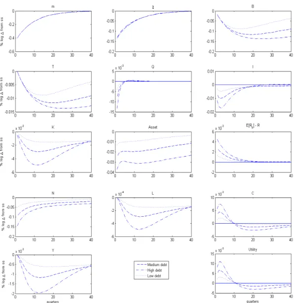
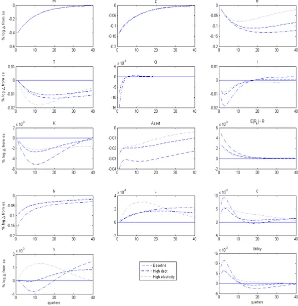
Figure 4 shows system dynamics following the default shock, for three different levels of steady state debt-to-GDP ratio, that also mean a different composition of banks’ asset side. We display the results for the most important financial and real variables.
5
Figure 4: Lump-sum taxes
Note: Low, medium and high debt represent, respectively, a steady state debt-to-GDP ratio of 40, 85 and 130% and a fraction debt-to-total banks’ assets of 6, 11 and 17%. Other variables such as GDP, consumption, investment and government spending and taxation have the same steady states in the three cases.
Summing up the results for lump-sum taxes in the baseline case, the model generates a decline in investment - and output - as a consequence of the debt restructuring process. This is associated to the leverage restriction faced by banks and to the loss of net worth they have after the shock. In terms of utility, there is a trade-off between short and long run utility, that mimics consumption path. In the next paragraphs we explain in details the dynamics of the shock for each agent in the economy.
financing requirement continues to fall, which means debt also falls further after initial shock. Taxes adjust to target debt to a steady state value, so once debt starts to fall, taxes are also reduced, depending on the elasticity parameter γ. Since government spending remains fixed for the whole simulation period, debt stock starts to recover after some time towards steady state level. As the defaultable fraction of debt at each period is being reduced as the shock diminishes, prices also recover and total value of debt assets in banks’ balance sheet rises again towards steady state.
The value of bonds in banks’ portfolio falls directly as a consequence of the shock, and so does total asset value. For the baseline calibration with debt-to-GDP ratio equal to 85%, the value of net worth falls by 9%, much more than the fall in the value of assets (2.5%). Weakening in balance sheet conditions and leverage restriction enforced by moral hazard constraint impose a deleveraging process for banks, inducing a fire sale of assets and a fall in demand for securities.
As a consequence of the drop in asset demand by banks, the spread of capital returns over the risk free rate rises, raising the costs for new capital acquisition. Tigther credit reduces private investment, and capital stock starts to decline. In a first moment, once output and government spending are intact, and once investment drops, consumption increases (there is a crowding-out effect between consumption and investment). In the banking sector, this is a reflection of the deleveraging process, in which banks do not take new deposits, and risk-free interest rates fall. So households face a lower demand for their savings and consume more in the present.
In the firm sector, decreasing capital stock reduces marginal product of labour, mean-ing that the wage rate that firms are willmean-ing to pay must be lower. As a consequence households supply less hours and output depresses further (labour has a higher weight in production function). Taxes are lump-sum and there is no wealth effect on labour supply (GHH preferences), so individuals become poorer but do not supply more hours in response. Besides, even though taxes decrease, they affect only total available wealth but do not influence marginal decisions to work or consume.
The initial debt repudiation of 40%, that lasts for a long period and leads to a haircut of around 11% in the lowest point of the path leads at the end to a fall in investment and output of, respectively, 1 and 0.12 %, in the lowest point of the path for the baseline case. Analysing the impact of default in terms of households’ utility, we see that it tends to mimic consumption path, because in this case response of labour has a lower order of magnitude. As consumption increases right after the shock, utility also goes up. In the long run, output drop leads to a contraction in consumption expenditures, which reflects on a negative deviation of utility in comparison to steady state. Utility remains lower for a long period, until output and consumption recovery is high enough.
Figure 4 shows that the higher the initial level of debt, the deeper the contraction in economic activity, since balance sheet effects are larger.
In comparison with the baseline calibration, raising initial debt level to 130% of GDP - a value that resembles the Greek case - amplifies investment and output fall to 1.6 and 0.2%, respectively. This amplified effect has roots in a deeper net worth contraction of almost 15% and a rise in financing costs.
When debt-to-GDP ratio is 40% and represents only 6% of total assets, the contrac-tion in investment in much less pronounced (0.45%) and leads to a contraccontrac-tion in GDP of 0.06%.
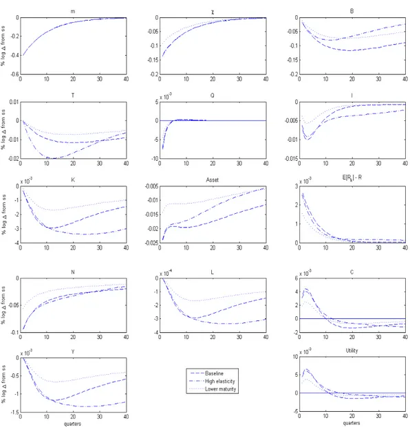
❼ Other cases: higher tax elasticity, longer maturity
We also analyse the impact of default in the model when parameters for elasticity of taxes with respect to debt and debt maturity are being changed. Graphic results are presented in Appendix.
When taxes respond more to debt deviation from steady state, government cuts taxes by a higher amount and hence debt level recovers faster, implying that government bonds’ value in banks portfolio recovers quicker. As banks deleverage, and this process is more flat and slow for higher elasticity, because debt value restores faster, banks tend not to shift a lot of demand from bonds to capital, leading the recovery in capital markets to take longer. Since recovery in capital markets is slower in this case, demand for labour by firms falls deeper and wages remain low for more time. Labour supply then remains shortened for a longer time.
This trade-off between banks portfolio effect and government budget constraint effect following a default episode suggests that fiscal consolidation - represented by a smaller reduction in taxes - might help investment markets recovery, in the absence of other de-fault costs that prevent debt restructuring.
Analysing the incidence of the shock to a context of longer average debt maturity, we see that the results resemble those of smaller debt. When a lower amount of debt should be repaid earlier, debt price decreases less after the shock and the haircut in debt level in the lowest point of the path is smaller. The effects on the tightening of credit conditions are also less pronounced, leading to a small fall in output.
5.2
Distortionary taxes
We now consider that government revenues are obtained through distortionary taxation over labour income, instead of lump-sum taxes. Government charges a rateτt over labour
Tt =τtWtLt (37)
τt=τw[1 +γ(Bt−B¯)] (38)
Where τw is a parameter calibrated to generate the same steady state tax revenue as
in the lump-sum case. On the household side, budget constraint and first order condition for labour supply become, respectively:
Ct+Dt+1=τtWtLt+ Πt+RtDt (39)
Lϕt = (1−τt)Wt (40)
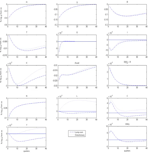
Figure 5: Lump-sum vs. Distortionary taxes
Note: Elasticity of taxes with respect to debt deviation remains the same in both cases as also does debt-to-GDP and debt-to-total assets. Steady state values for some real variables such as labour and output are lower for distortionary case, since tax rate over wage rents distorts labour supply decision.
This is actually the case for our baseline calibration. Even though capital stock is depressed by investment drop, workers now are willing to supply more labour because their net earnings from labour have increased by tax cuts. Once labour participation in output is twice the size of capital participation, and as both factors deviate from steady state in equivalent magnitudes (though with opposite signs), output increase from labour fully compensates decrease from capital in the short run, and output starts to rise after ten quarters. Hence labour response to distortionary taxes cushions depression in capital markets and alleviates output costs of default.
Utility comparison displays a trade-off between short and long run effects, because for distortionary taxes labour response has the same order of magnitude as consumption, thus affecting utility in the same proportion. Here the increase of labour supply in response to the shock works as a trade-off for utility. On the one side, labour increase contributes not to let output drop, hence keeping consumption higher. On the other side, a higher labour supply diminishes households’ utility in the long run. As the impulse-response functions make clear, the former effect is dominant, what leaves utility higher than in the case of lump-sum taxes.
❼ Distortionary taxes with higher tax elasticity and higher debt level
Figure 6: Distortionary taxes with higher debt level and higher tax elasticity
Note: In the baseline calibration, elasticity (γ) equals 0.1. For the high elasticity case, it is set to 0.25.
Debt level for is 80 and 130% of GDP for baseline calibration and high debt case, respectively.
6
Final Remarks
We have included a government sector that issues non-contingent debt hoarded by banks in a model of financial frictions, in order to explore the impact of a sovereign debt restruc-turing episode for the economy through the credit intermediation channel. Our model is different from most of the literature on sovereign defaults and debt crises, since we are dealing with a closed economy with a high debt-to-GDP ratio and banks that hold all this debt, instead of allowing for foreign creditors that may impose sanctions to governments that repudiate debt. Our model economy tries to resemble features of the Euroarea, con-sidering it as a big closed economy, since discussion about bailout schemes and default risk has been a central issue in the last years.
Results show that the model captures one important cost of default pointed out by empirical and theoretical literature on debt crises, namely the fall in investment that follows haircut episodes, what can be explained by a worsening in banks’ balance sheet conditions that limits credit for the private sector and raises their funding costs.
In terms of output decrease, this cost is though not significant enough to justify the existence of debt markets and the government incentives for debt repayment. Assuming that the government is able to alleviate its constrained budget by imposing a restructuring on debt repayment profile that allows it to cut taxes, our model generates an important difference for output path comparing lump-sum taxes and distortionary. For our calibra-tion, quantitative results show that is possible that the effect on labour supply generated by tax cuts dominates investment drop caused by credit crunch on financial markets.
Two important trade-offs arise from model results. The first one is between short and long run responses of consumption, output and utility to a default episode, mainly in the case of distortionary taxes. As seen in the previous section, labour response to distortionary taxes has the same order of magnitude as consumption deviations. Hence, a higher labour supply might prevent output and consumption drop in the long run, but at the disutility cost of supplying more hours. The second one comes from portfolio allocation by banks following the restructuring scheme. When taxes respond too much to debt contraction, debt face value recovers faster, banks do not shift much demand from sovereign markets, what delays adjustment in capital markets and output recovery.
References
[1] Andritzky, J. Government Bonds and their Investors: What are the facts and do they matter? IMF Working Paper, International Monetary Fund, n. 12/158, 2012.
[2] Arellano, C. Default risk and income fluctuations in emerging economies. American Economic Review, v. 98, n. 3, p. 690-712, 2008.
[3] Bernanke, B., & Gertler, M. Agency Costs, Net Worth, and Business Fluctuations.
American Economic Review, v. 79, n.1, 1989.
[4] Bernanke, B., Gertler, M., & Gilchrist, S. The Financial Accelerator in a quantitative Business Cycle Framework.Handbook of Macroeconomics, v. 3, 1999.
[5] Blanchard, O. & Kahn, C. The Solution of Linear Difference Models under Rational Expectations Econometrica, v. 48, n. 5, p. 1305-1311, 1980.
[6] Boissay, F., Collard, F. & Smets, F. Booms and systemic banking crises. European Central Bank Working Paper Series, European Central Bank, n. 1514, 2013.
[7] Bolton, P. & Jeanne, O. Sovereign default risk and bank fragility in financially inte-grated economies. NBER Working Paper Series. National Bureau of Economic Re-search, n. 16899, 2013.
[8] Borensztein, E. & Panizza, U. The Costs of Sovereign Default.IMF Working Papers, International Monetary Fund, n. 08/238, 2008.
[9] Broner, F., Martin, A. & Ventura, J. Sovereign Risk and Secondary Markets.American Economic Review, v. 100, n. 4, 2010.
[10] Brutti, F. Sovereign defaults and liquidity crises.Journal of International Economics, v. 84, n. 1, 2011.
[11] Bullow, J. & Rogoff, K. Sovereign Debt: Is to forgive to forget?.American Economic Review, v. 79, n. 1, 1989.
[12] Carlstrom, C., & Fuerst, T. Agency Costs, Net Worth, and Business Fluctuations: A Computable General Equilibrium Analysis. American Economic Review, v. 87, n. 5, 1997.
[13] Corsetti, G., Kuester, K., Meier, A., & M¨uller, J. Sovereign risk, fiscal policy and macroeconomic stability. The Economic Journal, v. 123, n. 566, 2013.
[15] De Bruyckere, V., Gerhardt, M., Schepens, G., & Vennet, R. Bank/Sovereign Risk Spillovers in the European Debt Crisis.Journal of Banking and Finance, v. 37, n. 12, 2013.
[16] Eaton, J., & Gersovitz, M. Debt with Potential Repudiation: Theoretical and Em-pirical Analysis. The Review of Economic Studies, v. 48, n. 2, 1981.
[17] Gertler, M. & Karadi, P. A model of unconventional monetary policy. Journal of Monetary Economics, v. 18, n. 1, p. 17-34, 2011.
[18] Gertler, M. & Kiyotaki, N. Financial Intermediation and Credit Policy in Business Cycle Analysis. in Friedman, B., & Woodford, M. (ed.), (2010). ”Handbook of Mon-etary Economics,” Handbook of MonMon-etary Economics, Elsevier, edition 1, v. 3, n. 3, 2010.
[19] Gertler, M., Kiyotaki, N. & Queralto, A. Financial Crises, Bank Risk Exposure and Government Financial Policy. Journal of Monetary Economics, v. 59, p. 14-34, 2012.
[20] Greenwood, J., Hercowitz, Z. & Huffman, G. Investment, Capacity Utilization and the Business Cycle. American Economic Review, v. 78, n. 3, 1988.
[21] Guerrieri, L., Iacoviello, M. & Minetti, R. Banks, sovereign debt and the international transmission of business cycles.NBER Working Paper, National Bureau of Economic Research, n. 18303, 2012.
[22] Guimaraes, B. Sovereign default: which shocks matter? Review of Economics Dy-namics, v. 14, n. 4, p. 553-576, 2011.
[23] Kiyotaki, N., & Moore, J. Credit Cycles Journal of Political Economy, v. 105, n. 2, 1997.
[24] Lojsch, D., Rodr´ıguez-Vives, M., & Slav´ık, M. The size and composition of govern-ment debt in the euro areaEuropean Central Bank Occasional Paper Series, European Central Bank, n. 132, 2011.
[25] Panizza, U., Sturzenegger, F., & Zettelmeyer, J. The Economics and Law of Sovereign Debt and Default. Journal of Economic Literature, v. 47, 2009.
[26] Popov, A., & Van Horen, N. The impact of sovereign debt exposure on bank lending: evidence from the European debt crisis.DNB Working Paper, De Nederlandsche Bank, n. 382, 2013.
A
Banks allocation problem
Using the conjecture for the value function form suggested in (26), we can write the Lagrangian for the banks’ maximization problem. Banks will maximize its terminal value (22) subject to the constraint (23).
L=νtQtKt+1+ζtχtBt+1+ηtNt−µt[λ(QtKt+1+ζtχtBt+1)−νtQtKt+1+ζtχtBt+1+ηtNt]
That can be simplified to
L = [νtQtKt+1+ζtχtBt+1+ηtNt] (1 +µt)−µtλ(QtKt+1+ζtχtBt+1) (41)
where µt is the Lagrangian multiplier with respect to the incentive constraint. The
first order conditions forKt+1, Bt+1 and µt are:
νt(1 +µt) =µtλ (42)
ζt(1 +µt) = µtλ (43)
λ(QtKt+1+ζtχtBt+1) =νtQtKt+1+ζtχtBt+1+ηtNt (44)
The first and second FOCs are symmetric. On the left hand side is the marginal benefit for the bank from expanding each of the assets components and on the right hand side the marginal cost of tightening the incentive constraint by λ. The last FOC is the incentive constraint itself.
The constraint binds (µt >0) only if the marginal discounted value of both the banks
assets is positive. In case the constraint binds, the FOCs for securities and bonds show that the discounted marginal value for each of those components should be equal. It means that in the margin, the bank is indifferent from investing resources in government bonds or private securities.
Now we show that the conjectured form of the value function holds. From (24), (25) and (26) we have:
νtQtKt+1+ζtχtBt+1+ηtNt=EtβΛt,t+1{(1−θ)Nt+1+θ[νt+1Qt+1Kt+2+ζt+1χt+1Bt+2+ηt+1Nt+1]}
Using the definitions of̟t and φt, we simplify the above equation to:
Inserting the definition of Ωt we get:
LHS=EtβΛt,t+1Ωt+1Nt+1
Substituting forNt+1:
LHS =EtβΛt,t+1Ωt+1[(Rkt+1−Rt+1)QtKt+1+ (Rbt+1−Rt+1)χtBt+1+Rt+1Nt]
Comparing the terms forKt+1,Bt+1andNt, we see that the conjecture holds if (28), (29), (27)
B
Other results
Figure 7: Lump sum taxes with longer maturity and higher tax elasticity