www.ann-geophys.net/25/2393/2007/ © European Geosciences Union 2007
Annales
Geophysicae
Electromagnetic energy deposition rate in the polar upper
thermosphere derived from the EISCAT Svalbard radar and
CUTLASS Finland radar observations
H. Fujiwara1, R. Kataoka2, M. Suzuki1, S. Maeda3, S. Nozawa4, K. Hosokawa5, H. Fukunishi1, N. Sato6, and M. Lester7
1Department of Geophysics, Graduate School of Science, Tohoku University, Sendai, Japan 2RIKEN (The Institute of Physics and Chemical Research), Saitama, Japan
3Faculty for the Study of Contemporary Society, Kyoto Women’s University, Kyoto, Japan 4Solar-Terrestrial Environment Laboratory, Nagoya University, Nagoya, Japan
5The University of Electro-Communications, Tokyo, Japan 6National Institute of Polar Research, Tokyo, Japan
7Department of Physics and Astronomy, University of Leicester, Leicester, UK
Received: 23 October 2006 – Revised: 5 October 2007 – Accepted: 14 November 2007 – Published: 29 November 2007
Abstract. From simultaneous observations of the European incoherent scatter Svalbard radar (ESR) and the Cooperative UK Twin Located Auroral Sounding System (CUTLASS) Finland radar on 9 March 1999, we have derived the height distributions of the thermospheric heating rate at the F re-gion height in association with electromagnetic energy inputs into the dayside polar cap/cusp region. The ESR and CUT-LASS radar observations provide the ionospheric parameters with fine time-resolutions of a few minutes. Although the geomagnetic activity was rather moderate (Kp=3+∼4), the electric field obtained from the ESR data sometimes shows values exceeding 40 mV/m. The estimated passive energy deposition rates are also larger than 150 W/kg in the upper thermosphere over the ESR site during the period of the en-hanced electric field. In addition, enhancements of the Ped-ersen conductivity also contribute to heating the upper mosphere, while there is only a small contribution for ther-mospheric heating from the direct particle heating due to soft particle precipitation in the dayside polar cap/cusp region. In the same period, the CUTLASS observations of the ion drift show the signature of poleward moving pulsed ionospheric flows with a recurrence rate of about 10–20 min. The esti-mated electromagnetic energy deposition rate shows the ex-istence of the strong heat source in the dayside polar cap/cusp region of the upper thermosphere in association with the day-side magnetospheric phenomena of reconnections and flux transfer events.
Keywords. Ionosphere (Ionosphere-atmosphere interac-tions; Polar ionosphere) – Magnetospheric physics (Polar cap phenomena)
Correspondence to: H. Fujiwara
1 Introduction
Various ionospheric and auroral phenomena due to the in-teraction between the solar wind and the magnetosphere have been observed in the dayside polar cap/cusp region. The polar patches, the pulsed ionospheric flows, and the poleward-moving radar auroral forms are well-known phe-nomena (e.g., Basu and Valladares, 1999; Provan et al., 1999; Wild et al., 2001, and references therein). In addition, travel-ing ionospheric disturbances (TIDs) caused by various forc-ings have been frequently observed in the polar cap region (e.g., Macdougall et al.,2001; Prikryl et al., 2005). These ionospheric and auroral phenomena indicate the presence of various energy inputs into the dayside polar cap/cusp region and heating processes for not only plasmas in the ionosphere but also neutrals in the thermosphere.
The variability of the convection electric field has been recognized to be one of the most important issues of the polar ionospheric/thermospheric physics since Codrescu et al. (1995) pointed out that the electric field fluctuation with time-scale of several minutes contributes to Joule heating. Codrescu et al. (2000) and Matsuo et al. (2002) derived bin-averaged maps of the electric field variability from incoher-ent scatter radar data and the Dynamics Explorer 2 (DE2) satellite data, respectively. Matsuo et al. (2002) used an em-pirical orthogonal function (EOF) analysis to show that the first two EOFs were related to the variability associated with the interplanetary magnetic field (IMF) and the third to the variability in the cusp region.
Fig. 1. The IMFBx, By, andBz components measured by the WIND spacecraft upstream in the solar wind, H-component of the geomagnetic field at Tromsø (TRO) and Longyearbyen (LYB) and the quick-look AE index on 9 March 1999, from top to bottom.
ionospheric convection and plasma flow: the region near the dayside dusk convection reversal boundary characterized by large (>1 km/s) and rapid (<2 min) fluctuations in line-of-sight velocity and the region at the higher latitudes in the con-vection throat characterized by relatively uniform flow over the polar cap at roughly 600 m/s. Using data obtained from the satellite CHAMP (Challenging Mini-satellite Payload) observations, L¨uhr et al. (2004) showed thermospheric den-sity enhancements of almost a factor of two at about 450 km altitude when the satellite passed the cusp region. They also found indications of enhanced small-scale field aligned currents observed simultaneously with the density enhance-ments and suggested atmospheric up-welling caused by local Joule heating in the cusp region.
These features of the electric field variations and/or the small-scale field aligned currents suggest electromagnetic energy deposition which results in various dynamical pro-cesses in the dayside polar cap/cusp region. Maeda et al. (2002, 2005) showed that the dayside E region ion and neutral temperatures at Longyearbyen were higher than those
at Tromsø with the European incoherent scatter (EISCAT) radars. They suggested the heat transport by the polar neu-tral winds in addition to Joule and/or auroral particle heating for causing the high temperatures in the polar cap/cusp E re-gion. Fujiwara et al. (2004) estimated the electromagnetic and turbulent energy dissipation rates in the lower thermo-sphere using the EISCAT Svalbard radar (ESR) at Longyear-byen. They showed that, on the average, the electromagnetic and turbulent energy dissipations were dominant above and below about 110 km, respectively. The energetics of neutral gases in the E region/lower thermosphere has been often in-vestigated (e.g., Fujii et al., 1999; Thayer, 2000), while stud-ies of the F region/upper thermosphere were quite few (e.g., Wu et al., 1996; Thayer and Semeter, 2004).
In this study, we focus our attention on the electromag-netic energy input from the magnetosphere into the dayside polar cap/cusp region of the upper thermosphere. In order to observe the ionosphere with fine time-resolutions, the ESR and the Cooperative UK Twin Located Auroral Sounding System (CUTLASS) Finland radar have been used because these radars provide the ionospheric parameters with time-resolutions of a few minutes. Simultaneous observations with the ESR and CUTLASS are quite useful for studying origins of ionospheric/thermospheric variations at the F re-gion height (e.g., Ogawa et al., 2001; Wild et al., 2001).
In the present study, the CUTLASS Finland radar observes the signatures of cusp plasma and poleward moving pulsed ionospheric flows during the period of the significant ther-mospheric heating observed with the ESR, suggesting a rela-tionship between the thermospheric heating and the dayside magnetospheric phenomena. The height profiles of the neu-tral gas heating rate due to the electromagnetic energy de-position are presented, and the contributions of the particle precipitation, neutral density, and neutral wind in the cusp region to heating the upper thermosphere are also discussed in the following sections.
2 Observational condition and locations of radar sites
We investigate energy inputs into the dayside polar cap/cusp region during 06:00–12:00 UT on 9 March 1999. The indices for representing the solar and geomagnetic activities were as follows: F10.7=125×10−22W/m2/Hz and Kp=3+∼4 (Ap=21). The interplanetary magnetic field (IMF)By and
Bzcomponents were predominantly negative for this period. Although the variations of the IMF and the geomagnetic field in this period were already shown (Maeda et al., 2002; 2005), the variations are shown again in Fig. 1. Before 06:00 UT, prominent IMF variations, which caused the magnetic field variations at Longyearbyen, are seen in the IMFBx,Byand
on the period of 06:00–12:00 UT when the IMF has small fluctuations after the large variations.
The ESR site at Longyearbyen, Svalbard is located at 78.09◦N, 16.03◦E (75.12◦N, 113.00◦E in geomagnetic co-ordinates). The local solar time (LST) and the magnetic local time (MLT) at Longyearbyen are approximately UT + 1 and UT + 3, respectively. Figure 2 indicates the location of the ESR site and the beam directions of the CUTLASS Finland radar in the geomagnetic latitude and MLT coordinate sys-tem. The field of view of the CUTLASS Finland radar con-sists of 16 beams (Beam 0–15), with Beam 9 over the ESR site.
Figure 3 shows the high latitude electric potential de-scribed with the Heppner-Maynard empirical electric con-vection field model (Heppner and Maynard, 1987) in the ge-omagnetic latitude and MLT coordinate system when IMF
ByandBzare negative. The locations of the ESR site in the period between 06:00 and 12:00 UT (09:00 and 15:00 MLT at Longyearbyen) are shown by circle dots with numbers in-dicating UT. The pattern of the electric field at the ESR site inferred from the empirical model is approximately consis-tent with that obtained from the ESR observations. The elec-tric field obtained from the ESR observations is shown in the following section. In the present case, the recent electric po-tential model developed by Weimer (2005) shows a similar pattern to the Heppner-Maynard model (see e.g., Fig. 2 of Weimer, 2005). The ESR site seems to be at around the day-side convection reversal boundary of the dusk convection cell and/or poleward of the auroral oval during the period.
3 Observational results
3.1 ESR observations
The ESR allows us to observe the ionosphere connected to several magnetospheric regions, e.g., the polar cap and cusp region, in the height range from about 100 to several hun-dreds of km. The details of the radar system were described by, e.g., Wannberg et al. (1997). In the present study, we use the EISCAT Common Program 2 (CP-2) mode version L data obtained in the period of 06:00–12:00 UT on 9 March 1999. Some of the data were already presented by Maeda et al. (2002, 2005). The details of the ESR observation and the method for derivation of the ionospheric parameters are de-scribed in these papers. The ionospheric conductivity tensor is also derived from the ESR data assuming ion and neutral compositions, collision frequency between ions and neutrals, and that between electrons and neutrals in the same way as Fujiwara et al. (2004). We use data obtained from the vertical beam observations to derive the vertical profiles of the elec-tron density and temperature over the ESR site. The methods for derivation of the ionospheric parameters (quantities) are briefly mentioned here.
Fig. 2. Location of the ESR site at Longyearbyen (circle dot) and the field of view of the CUTLASS Finland radar in the geomagnetic latitude and MLT coordinate system. The field of view of the CUT-LASS Finland radar consists of 16 beams (Beam 0-15), with Beam 9 over the ESR site.
Fig. 3. High latitude electric potential calculated by using the Heppner-Maynard electric convection field model in the condition that IMF By and Bz are negative. The locations of the ESR site during 06:00–12:00 UT are marked by circle dots with numbers in-dicating the universal time.
Fig. 4. The derived electric field during 04:00–12:00 UT on March 9, 1999 from the ion velocity at 278 km assuming that theE×B force drives motions of ions and electrons. The meridional (solid lines) and zonal (dotted lines) components of the electric field are positive toward the north and east, respectively.
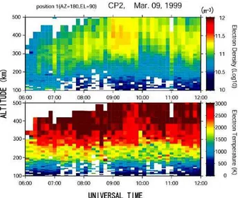
Fig. 5. The electron density (upper) and temperature (lower) de-rived from the ESR observations during 06:00–12:00 UT. Note that the electron density is displayed with logarithmic scale.
the ion velocity at about 278 km assuming that the E×B
force drives motions of ions and electrons,
E= −(Vi ×B)278, (1) whereBis the magnetic field. The value of the electric field is derived by combining the measurements of long pulse F region monostatic ion velocity with estimates of the mag-netic field described by International Geomagmag-netic Refer-ence Field (IGRF) model [International Association of Ge-omagnetism and Aeronomy Division I Working Group 1, 1987]. The errors of the electric field are estimated only from those of the ion velocity which are derived from IS spectrum fitting procedures. The errors due to spatial inhomogeneity are not considered here. The average absolute value of the electric field,|E|, and the error,δ|E|, are 35.7 and 2.5 mV/m, respectively in the period of 06:00–12:00 UT. The average of
the relative error,δ|E|/|E|, is estimated to be 6.9 % in the present case. Furthermore, the average of the relative error ofE2,δ(E2)/E2(=2δ|E|/|E|), is 14%.
Figure 4 shows the electric field obtained by using Eq. (1). The meridional (solid lines) and zonal (dotted lines) compo-nents of the electric field are positive toward the north and east, respectively. In the period of 06:00–12:00 UT, the elec-tric field is almost in the south-east direction except for some intervals, in particular during 08:14–08:30 UT.
Figure 5 shows the electron density (upper panel) and tem-perature (lower panel) derived from the ESR observations. Note that the electron density is displayed with logarithmic scale in units of m−3. The electron density gradually in-creases with the course of the local solar time particularly above about 300 km altitude. The large increases in the elec-tron density are seen during about 07:30–11:00 UT (08:30– 12:00 LST or 10:30–14:00 MLT at Longyearbyen) above about 300 km height with some cessations, which implies enhancements of precipitating soft electrons during this pe-riod. The enhancements of the electron temperature (>2500– 3000 K) are also seen above about 300 km altitude. The en-hancements of the electron density and temperature almost correspond to each other.
Figure 6a–c show the strength of the electric field,|E|, the Pedersen conductivity,σP, and the passive energy deposition rate per unit mass,σPE2/ρ, derived from the ESR data, re-spectively, whereρis the atmospheric density obtained from the MSISE-90 empirical model (Hedin, 1991). The Pedersen conductivity,σP ,is calculated from Eq. (2),
σP =
ene
B
νenωe
ω2 e+νen2
+ νinωi
ω2i +νin2
!
, (2)
whereeis the electron electrostatic charge,neis the electron or plasma density derived from observations,νenis the colli-sion frequency between electrons and neutrals,νinis the col-lision frequency between ions and neutrals,ωeis the electron cyclotron frequency, andωiis the ion cyclotron frequency. It is noted that the Pedersen conductivity is shown in the height range between 290 and 490 km, andσPE2/ρ between 100 and 500 km.
Fig. 6. (a) The strength of the electric field,|E|, (b) the Pedersen conductivity above 290 km, and (c) the passive energy deposition rate per unit mass,σPE2/ρ, obtained from the ESR observations during 06:00–12:00 UT.Eis the electric field,σP is the Pedersen conductivity, andρ is the neutral mass density obtained from the MSISE-90 empirical model.
maximum value at around 120 km altitude depending on the Pedersen conductivity profile,σpE2/ρshows large values in the upper thermosphere because of lower neutral density in the upper thermosphere than that in the lower thermosphere. Since it would be helpful to have quantities in units of W/m3 for comparison with other studies, we show both the values in units of W/kg and W/m3.
There are some occurrences of large heating rates (>150 W/kg) at the following approximate altitudes and times: e.g., 171 W/kg (8.16×10⁻¹⁰W/m3) at 385 km and 08:38 UT, 177 W/kg (4.53×10⁻¹⁰W/m3) at 421 km and 09:18 UT, 320 W/kg (2.56×10⁻¹⁰W/m3) at 493 km and 10:06 UT, 249 W/kg (1.19×10⁻⁹W/m3) at 385 km and 10:38 UT. The heating rate strongly depends on the elec-tric field. In particular, the enhancements of the elecelec-tric field between about 08:00 and 11:00 UT correlate well with the large heating rates. As seen in Fig. 6b, the Pedersen con-ductivity increases after about 09:00 UT corresponding to the enhancements of the electron density. The increases in the Pedersen conductivity also contribute to the large heating rates together with the enhanced electric field.
Fig. 7. (a) The Pedersen conductivity,σP and (b) passive energy deposition rate,σPE2/ρ, at about 350 km altitude obtained from the ESR observations during 06:00–12:00 UT. These are the same as those shown in Fig. 6 except for line plots at a specific height.
In order to clarify the enhancements ofσp andσpE2/ρ, line plots of their variations at about 350 km altitude are shown in Fig. 7a and b, respectively. During about 08:30– 11:00 UT, enhancements of the heating rate are seen in Fig. 7b. Enhancements of the conductivity are also remark-able during about 09:00–09:50 UT as shown in Fig. 7a. The enhancements of the heating rate at 08:38, 10:06, and 10:38 UT are due to enhancements of the electric field, while the enhancements of the heating rate during about 09:00– 09:50 UT are due to enhancements of both the conductivity and electric field as mentioned above.
3.2 CUTLASS observations
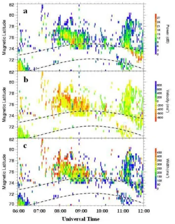
Fig. 8. (a) The echo power, (b) line-of-sight ion Doppler velocity, and (c) spectral width obtained from the Beam 9 observations dur-ing 06:00–12:00 UT (09:00–15:00 MLT at Longyearbyen) in the 70◦–82◦geomagnetic latitude range. The dashed lines denote the northward and southward edges of the Feldstein statistical auroral oval atKp=4. The positive (negative) values of the ion Doppler velocity indicate the motions toward (away from) the radar site, namely, equatorward (poleward) flows.
this study, we show the observational data from Beam 9 (over the ESR site) every 2 min.
Figures 8a-c show temporal variations of the echo power, line-of-sight ion Doppler velocity, and spectral width ob-tained from the Beam 9 observations, respectively. The ordi-nate and abscissa shown in Fig. 8 are the geomagnetic lati-tude and the universal time, respectively. The dashed lines in each panel show the locations of the poleward and equator-ward edges of the Feldstein statistical auroral oval (Feldstein and Starkov, 1967) atKp=4 as a function of the universal time. Note that Longyearbyen is located at 75.12◦ in geo-magnetic latitude which is at the north of the statistical auro-ral oval during 06:00–12:00 UT. The positive (negative) val-ues of the ion Doppler velocity indicate the motions toward (away from) the radar site, namely, equatorward (poleward) flows.
The signature of the pulsed ionospheric flows (PIFs) mov-ing away from the radar site, i.e., the quasi-periodic variation of the high-speed plasma motion (>600 m/s) away from the
Fig. 9. The calculated heating rates (W/kg) due to precipitating electrons (dotted line), protons (dashed line), both particles (solid line labeled QP), andσpE2/ρat 09:10 UT derived from the ESR observations (dashed-dotted line labeled QJ).
radar site, is detected during about 07:30–10:10 UT (10:30– 13:10 MLT at and poleward of Longyearbyen) as seen in Fig. 8b. The recurrence rate seems to be about 10–20 min. A similar variation is also seen in the spectral width (Fig. 8c). The high-speed plasma motions more than 800 m/s, which correspond to the electric field more than 36 mV/m, observed during about 08:00–09:20 UT and at around 10:10 UT are consistent with large heating rates or strong electric field ob-tained from the ESR observation. Sudden and large change in the flow direction is seen at around 08:30 UT and 75◦ ge-omagnetic latitude, corresponding to change in the electric field (form southward to northward) shown in Fig. 4. In ad-dition, quasi-periodic enhancements of the ionospheric flows at around 07:50–08:00, 08:20–08:30, 08:30–08:50, 09:00– 09:10, 09:10–09:20, and 10:10 UT almost correspond to peaks of the electric field strength shown in Fig. 6a.
SuperDARN observation in the cusp region. Furthermore, the Defense Meteorological Satellite Program (DMSP) F11 satellite observed the cusp-type ion precipitation over Sval-bard during 09:10–09:11 UT (see Maeda et al., 2002) when the wide spectral width is seen in Fig. 8c. The enhanced elec-tron density and temperature observed with the ESR are also consistent with the ionospheric signature of the cusp region (e.g., Watermann et al., 1992). These suggest that Svalbard was located in or in the vicinity of the cusp region in the pe-riod of the high-speed ion flows (07:30–10:10 UT).
3.3 Comparison of the particle heating rate with the Passive energy deposition rate
In order to evaluate a relative importance ofσpE2/ρto the to-tal energy deposition rate, we also estimate the particle heat-ing rate in the cusp region with the calculation method pre-sented by Rees (1963, 1982) using the atmospheric density obtained from the MSISE-90 model. The ionization rates due to precipitating electrons,Qe, and ions,Qi, are calculated by using the following Eqs. (3) and (4), respectively,
Qe
F =qz = E0
1ε ρ(z)
R λ(Z/R), (3)
Qi
F =qz= EP
1ε ρR
R n(M)z
n(M)R
λ(Z/R)fion, (4) whereF is the flux of incident electrons or ions per unit area, E0 and Ep are initial energies of incident electrons and ions, respectively,1εis the energy loss per ionization, taken as 35 eV,λis the normalized energy dissipation distri-bution function, Z/R is the fractional depth of penetration (R
is the maximum penetration depth of the electrons or ions). In Eq. (4)ρR is the atmospheric density at the height of the maximum ion penetration, andn(M)z and n(M)R are the effective number densities at atmospheric depths of z and
R, respectively. See Rees (1963, 1982) and Millward et al. (1999) for details. Using the above ionization rates and the heating efficiency,ε, the atmospheric heating rate,QP, is calculated as (see Rees et al., 1983),
QP =
q(E)·ε
ρ 1ε·e·F (E)=
Q(E)·ε
ρ 1ε·e. (5)
Both precipitating ions and electrons are assumed to have Maxwellian flux spectra with energy ranges between 0– 20 keV and 0–5 keV, respectively. Since Eq. (5) describes the heating rate for mono-energetic particles, we calculate integration of Eq. (5) over the energy range assuming above in both cases of electrons and ions. Based on the DMSP F11 satellite observation during 09:10–09:11 UT, we also as-sume the incident electrons with the maximum differential flux of 1.00×10⁹eV cm−2s−1sr−1eV−1at the mean energy of 0.1 keV whilst ions with the maximum differential flux of 1.00×10⁸eV cm−2s−1 sr−1 eV−1 at the mean energy of 1 keV. These spectra have the same mean energies and similar
maximum differential fluxes as those assumed by Millward et al. (1999). The work by Millward et al. (1999) was based on the DMSP satellite observations of the cusp region pre-sented by Newell et al. (1991). Figure 9 shows the calculated heating rates (W/kg) due to precipitating electrons (dotted line), protons (dashed line), and both particle species (solid line labeledQP). The neutral gas heating efficiency is ob-tained from Rees et al. (1983). The profile ofσPE2/ρ at 09:10 UT derived from the ESR observations is also plotted in Fig. 9 (dashed-dotted line labeledQJ).
The peak altitude of the particle heating rate is 370 km, which is almost the same as that of σPE2/ρ of 385 km. The peak magnitude of the particle heating rate is only 8.62 W/kg (5.11×10⁻¹¹W/m3), much less than that of
σPE2/ρ(144 W/kg or 6.86×10⁻¹⁰W/m3). The precipitating soft electrons would contribute to heating through enhance-ment of the Pedersen conductivity rather than direct parti-cle heating in the polar cap/cusp region of the upper thermo-sphere.
Wu et al. (1996) calculated the Joule and particle heating rates in the cusp region including effects of the modeled neu-tral wind with a one-dimensional satellite track model and the DE2 satellite particle data. They also showed that the Joule heating rate was greater than the particle heating rate at all altitudes below the satellite.
4 Discussion
From a thermospheric general circulation model simulation, Killeen and Roble (1986) showed that parcels transiting the dayside cusp were heated due to soft particle precipitation and this energy was then advected over the polar cap. In contrast to the present result, they estimated a small Joule heating rate because they assumed the small empirical con-vection electric field in the cusp region. In order to highlight the dynamical and thermodynamical effects of the localized cusp heating, they assumed large energy inputs due to precip-itating soft particles 5-10 times larger than the typical ones (see Killeen and Roble, 1986). Their scenario for heating the polar cap thermosphere by means of the cusp energy will become more realistic when we consider the large electro-magnetic energy deposition into the cusp region as shown in the present study.
We have estimated the passive energy deposition rate
σpE2instead of the electromagnetic energy transfer rateJ·E neglecting the effects of the neutral wind since there are no observational data for the dayside neutral wind at the F re-gion height in the present study. We evaluate the importance of the neutral wind on the electromagnetic energy deposition with the ratio ofJ·EtoσpE2.
The ratio,R, ofJ·E(∼σp·(E+U×B)·E) toσpE2is rep-resented as,
R=J·E
σPE2
∼ σP ((E+U×B)·E)
σPE2
=1+(U×B)·E
Fig. 10. Global pattern of the horizontal neutral wind derived from HWM-93 at 400 km altitude and 10:00 UT (30◦and 210◦ longi-tudes are noon and midnight, respectively) on 9 March in the con-dition ofF10.7=125 andAp=21. The maximum arrow indicates the wind velocity of 359 m/s.
Fig. 11. Schematic illustration which shows a relationship between the neutral windU, electric fieldE, andU×Bin the northern high latitude region in cases; (a)Ublows in the direction opposite toE and (b)Ublows in the direction perpendicular toE.
The neutral wind velocity,U, seems to be mostly less than 500 m/s in the polar cap/cusp region (e.g., Hays et al., 1984). In particular, the empirical neutral wind model of HWM-93 (Hedin et al., 1996) shows winds less than 300 m/s in the northern dayside high-latitude region in the present condi-tion. Figure 10 shows the global pattern of the horizontal neutral wind derived from HWM-93 at 400 km altitude and 10:00 UT (30◦and 210◦longitudes are noon and midnight, respectively) on 9 March in the condition ofF10.7=125 and
Ap=21. The maximum arrow indicates the wind velocity of 359 m/s. The meridional winds presented by HWM-93 have the northward component in the northern dayside high-latitude region. We therefore consider only the northward winds in the meridional direction in the following discussion. Figure 11a and b are schematic illustrations which show relationships between the neutral windU, electric fieldE, and U×B. Since the electric field E was predominantly south-eastward in the present case, Fig. 11a and b show such a case. WhenU is north-westward (opposite toE),U×B
is perpendicular toE(Fig. 11a). In this case,J·Eequals to
σpE2, namelyR=1 (see Eq. 6). WhenU is north-eastward (perpendicular toE),U×Bis opposite toE (Fig. 11b). In this case,U contributes to reducing the electromagnetic en-ergy deposition in the thermosphere most effectively.
As seen in Fig. 10, U tends to blow in the north-west direction during 07:00–13:00 LST (09:00–15:00 MLT at Longyearbyen) in the northern high-latitude region. The con-tribution ofUfor reducing the electromagnetic energy depo-sition seems to be small during this time interval. In general, the direction of the zonal winds may be variable depending on the local ion-drag and pressure gradient forces. Assuming thatU is 500 m/s (chosen as a rigid condition for the elec-tromagnetic energy deposition in the present case, see, e.g., Hays et al., 1984) and thatBis perpendicular toUwith mag-nitude of 4.58×10⁻⁵T (based on the value calculated with the IGRF model which also presents the magnetic inclination of 82.1◦over Svalbard at 400 km altitude), the value ofU×B
is obtained to be 22.9 mV/m. The zonal and meridional com-ponents of the electric field were about 47.0 (eastward) with error of 1.7 and−67.5 (southward) with error of 3.9 mV/m, respectively, when the maximum passive energy deposition rate is obtained at 10:06 UT. WhenU contributes to reduc-ing the electromagnetic energy deposition most effectively, namely,U×B is opposite toE (U blows in the north-east direction when E is south-eastward), R is estimated to be 0.722 from Eq. (6). SinceσpE2/ρ is estimated to be about 320 W/kg at 10:06 UT, the electromagnetic energy transfer rate is derived as J·E/ρ=σpE2/ρ·R=320·0.722=231 W/kg (1.84×10⁻¹⁰W/m3). The electromagnetic energy more than about 70% ofσpE2/ρwould deposit in and/or in the vicinity of the cusp region even when the strong neutral wind con-tributed to reducing the deposition rate.
From the CHAMP observations, Liu et al. (2005) showed that the MSISE-90 model underestimated the thermospheric density at 400 km altitude of about 20–30% in the cusp re-gion while the observations outside the cusp rere-gion were in good agreement with the MSISE-90 predictions. The present estimation of the heating rates per unit mass may be overestimated due to the possible underestimation of the MSISE-90 model density. Owing to the underestimation of the thermospheric density by about 30% including the neu-tral wind effect, the electromagnetic energy transfer rate,
J·E/ρ, is estimated to be at lowest 178 W/kg (=231/(1+0.3) W/kg ∼1.43×10⁻¹⁰W/m3) at 10:06 UT. Furthermore, if we consider the error for the electric field, the relative er-ror of δ(E2)/E2 is estimated to be 10.3% at 10:06 UT. Consequently, the possible J·E/ρ more than about 50– 60% (∼178×0.897/320×100 or 178×1.103/320×100) of
σpE2/ρestimated from the ESR data is expected even when we consider the neutral wind effect, mass density ambiguity, and the error of the electric field.
Fig. 6 in their paper). These values correspond to the rates per unit mass of 13 and 32 W/kg, respectively, which are much less than the present result of 160 (=178×0.897)−196 (=178×1.103) W/kg. The heating rate of 160–196 W/kg is also larger than the zonally averaged Joule heating rate with the maximum value of about 86 W/kg in the auroral oval during the geomagnetically disturbed period (Maeda et al., 1989).
Wu et al. (1996) estimated the Joule and particle heat-ing rates in the cusp region usheat-ing a one-dimensional satel-lite track model with the DE2 satelsatel-lite data in representative cases for active (19 September, 1981;Kp=5) and quiet (23 September, 1981;Kp=1) geomagnetic conditions. The cal-culated Joule heating rate was greater than the particle ing rate at all altitudes below the satellite and the Joule heat-ing peaked on the poleward side of the cusp/cleft precipita-tion region. Their estimates of the Joule heating rates were about 1.6×10⁻⁷ergs cm−3s−1in active and about 1.0×10⁻⁷ ergs cm−3s−1in quiet geomagnetic conditions at 385 km al-titude (see figures in their paper). Using the atmospheric den-sity of the MSISE-90 model, the heating rates per unit mass are estimated to be about 1.3×10³W/kg and 1.2×10³W/kg in the two cases, respectively. In the geomagnetically ac-tive period, the particle heating rate and the Joule heating rate outside the cusp are also estimated to be about 26 and 75 W/kg, respectively, from their results.
The previous TGCM simulations seem to underestimate the Joule heating rate because of the fluctuation of the elec-tric field as pointed by Codrescu et al. (1995), particularly in the cusp region. Codrescu et al. (1995) pointed out that their GCM calculations underestimated the Joule heating rate by about 30 %. On the other hand, the DE 2 and ESR obser-vations indicate the importance of the Joule heating in the cusp or in the dayside polar cap region. The discrepancy of the estimated heating rates between Wu et al. (1996) and the present study seems to be mainly caused by the difference of the Pedersen conductivities between the works. Wu et al. (1996) calculated the ion composition and electron den-sity to derive the Pedersen conductivity using the particle data obtained from the DE 2 observation, while we used the electron density profile obtained from the ESR observations and assumed ion composition from an empirical model. Be-cause validation work on the satellite track model by Deng et al. (1995) showed that the Joule heating rate and electron density in the F region were overestimated comparing with those derived from the Chatanika radar observations, there is a possibility that Wu et al. (1996) overestimated the Ped-ersen conductivity and the Joule heating rate at the F region height. This suggests that the Pedersen conductivity is also important in addition to the fluctuation of the electric field for estimation of the Joule heating rate at the F region height. The present study suggests large electromagnetic energy deposition rates in, and/or, in the vicinity of the cusp region in the upper thermosphere. It should be noted here that many previous studies, in particular GCM studies, used the
time-averaged electric field (e.g., hourly time-averaged one) while the present results are obtained from the ESR data with fine time-resolutions. The present electromagnetic energy deposition rate also suggests the existence of the strong heat source in the dayside polar cap/cusp region of the upper thermo-sphere in association with the dayside magnetospheric phe-nomena of reconnections and flux transfer events. This heat source/energy input can be a possible source for generating disturbances in the thermosphere/ionosphere as well as TIDs originated from the Alv´enic IMF-By oscillations as shown by Prikryl et al. (2005).
5 Conclusions
In order to investigate electromagnetic energy inputs into the dayside polar cap/cusp region of the upper thermosphere, we have focused on significant thermospheric/ionospheric heat-ing events on 9 March 1999, observed simultaneously with the ESR and the CUTLASS Finland radar.
During about 07:30–10:10 UT, the CUTLASS radar ob-served the signatures of the cusp plasma and the pulsed iono-spheric flows (PIFs): the wide spectral width and the quasi-periodic variation (with the recurrence rate of∼10–20 min) of the high-speed plasma motion (>600–800 m/s) away from the radar site. The pulsed ionospheric flows are the iono-spheric signature of the flux transfer events (FTEs).
The ESR observation showed the electron density and temperature enhancements above about 300 km during about 07:30–11:00 UT. Large passive energy deposition rates,
σpE2/ρ, of more than 150 W/kg have been obtained during the period of the large electric field which sometimes showed values exceeding 40 mV/m. In addition to the electric field enhancements, the Pedersen conductivity enhanced by the precipitating soft electrons also contributed to heating in the cusp region, while the direct heating due to the particle pre-cipitation would be small. The maximum heating rate has been estimated asσpE2/ρ=320 W/kg at about 493 km alti-tude at 10:06 UT. Even when we take into account the neu-tral wind effect, ambiguity of the neuneu-tral mass density, and the maximum error of the electric field, the possibleJ·E/ρ
more than 160 W/kg (∼50% ofσpE2/ρ)is expected from the above heating rate.
Acknowledgements. We are indebted to the Director and staff of EISCAT for operating the facilities and supplying the data. EIS-CAT is jointly funded by the Particle Physics and Astronomy Re-search Council (UK), Centre National de la Recherch´e Scientifique (France), Max-Plank Gesellschaft (F.R.G.), Suomen Akatemia (Finland), National Institute of Polar Research (Japan), Norges Almenvitenskapelige Forskningsrad (Norway), and Naturveten-skapliga Forskningsradet (Sweden). CUTLASS is deployed and operated by the University of Leicester, and is jointly funded by the UK Particle Physics and Astronomy Research Council, the Finnish Meteorological Institute, and the Swedish Institute of Space Physics. Thanks also to the staff of CDA web, and WDC-C2, Kyoto University for providing public WIND satellite data and geomag-netic indices, respectively. The IMAGE data was kindly supplied by the Auroral Observatory, University of Tromsø. The empirical mod-els of MSISE-90 and HWM-93 are provided by NSSDC/NASA. This work was supported in part by Grant-in-Aid for Scientific Re-search and the 21st Century COE program “Advanced Science and Technology Center for the Dynamic Earth” by the Ministry of Edu-cation, Science, Sports and Culture, Japan. The joint research pro-gram of the Solar-Terrestrial Environment Laboratory, Nagoya Uni-versity also supported a part of this work.
Topical Editor M. Pinnock thanks two anonymous referees for their help in evaluating this paper.
References
Baker, K. B., Dudeney, J. R., Greenwald, R. A., Pinnock, M., Newell, P. T., Rodger, A. S., Mattin, N., and Meng, C.-I.: HF-radar signatures of the cusp and low latitude boundary layer, J. Geophys. Res., 100, 7671–7696, 1995.
Basu, S. and Valladares, C.: Global aspects of plasma structures, J. Atmos. Sol.-Terr. Phy., 61, 127–139, 1999.
Codrescu, M.V., Fuller-Rowell, T. J., and Foster, J. C.: On the importance of E-field variability for Joule heating in the high-latitude thermosphere, Geophys. Res. Lett., 22, 2393–2396, 1995.
Codrescu, M. V., Fuller-Rowell, T. J., Foster, J. C., Holt, J. M., and Cariglia, S. J.: Electric field variability associated with the Millstone Hill electric field model, J. Geophys. Res., 105, 5265– 5274, 2000.
Deng, W., Killeen, T. L., Burns, A. G., Johnson, R. M., Emery, B. A., Roble, R. G., Winningham, J. D., and Gary, J. B.: One-dimensional hybrid satellite track model for the Dynamics Ex-plorer 2 (DE 2) satellite, J. Geophys. Res., 100, 1611–1624, 1995.
Feldstein, Y. I. and Starkov, G. V.: Dynamics of auroral belt and polar geomagnetic disturbance, Planet. Space Sci., 15, 209–229, 1967.
Fujii, R., Nozawa, S., Buchert, C. S., and Brekke, A.: Statistical characteristics of electromagnetic energy transfer between the magnetosphere, the ionosphere, and the thermosphere, J. Geo-phys. Res., 104, 2357–2366, 1999.
Fujiwara, H., Maeda, S., Suzuki, M., Nozawa, S., and Fuku-nishi, H.: Estimates of electromagnetic and turbulent energy dissipation rates under the existence of strong wind shears in the polar lower thermosphere from the EISCAT Sval-bard Radar observations, J. Geophys. Res., 109, A07306, doi:10.1029/2003JA010046, 2004.
Greenwald, R. A., Baker, K. B., Dudeney, J. R., Pinnock, M., Jones, T. B., Thomas, E. C., Villain, J.-P., Cerisier, J.-C., Senior, C., Hanuise, C., Hunsucker, R. D., Sofko, G. J., Koehler, J., Nielsen, E., Pellinen, R., Walker, A. D. M., Sato, N., and Yamagishi, H.: DARN/SuperDARN: a global view of the dynamics of high-latitude convection, Space Sci. Rev., 71, 761–796, 1995. Hays, P. B., Killeen, T. L., Spencer, N. W., Wharton, L. E., Roble,
R. G., Emery, B. A., Fuller-Rowell, T. J., Rees, D., Frank, L. A., and Craven, J. D.: Observations of the dynamics of the polar thermosphere, J. Geophys. Res., 89, 5597–5612, 1984.
Hedin, A. E.: Extension of the MSIS thermosphere model into the middle and lower atmosphere, J. Geophys. Res., 96, 1159–1172, 1991.
Hedin, A. E., Fleming, E. L., Manson, A. H., Schmidlin, F. J., Av-ery, S. K., Clark, R. R., Franke, S. J., Fraser, G. J., Tsuda, T., Vial, F., and Vincent, R. A.: Empirical wind model for the upper, mid-dle and lower atmosphere, J. Atmos. Terr. Phy. 58, 1421–1447, 1996.
Heppner, J. P. and Maynard, N. C.: Empirical High-Latitude Elec-tric Field Models, J. Geophys. Res. 92, 4467–4489, 1987. IAGA Division I Working Group 1, International geomagnetic
ref-erence field revision 1987, J. Geomag. Geoelectr., 39, 773–779, 1987.
Killeen, T. L. and Roble, R. G.: An analysis of the high-latitude thermospheric wind pattern calculated by a thermospheric gen-eral circulation model 2. Neutral parcel transport, J. Geophys. Res., 91, 11 291–11 307, 1986.
Liu, H., L¨uhr, H., Henize, V., and K¨ohler, W.: Global distribution of the thermospheric total mass density derived from CHAMP, J. Geophys. Res., 110, A04301, doi:10.1029/2004JA010741, 2005. L¨uhr, H., Rother, M., K¨ohler, W., Ritter, P., and Grunwaldt, L.: Thermospheric up-welling in the cusp region: Evidence from CHAMP observations, Geophys. Res. Lett., 31, L06805, doi:10.1029/2003GL019314, 2004.
Macdougall, J. W., Andre, A. D., Sofko, G. J., Huang, C.-S., and Koustov, A. V.: Travelling ionospheric disturbance properties deduced from Super Dual Auroral Radar measurements, Ann. Geophys., 18, 1550–1559, 2001,
http://www.ann-geophys.net/18/1550/2001/.
Maeda, S., Fuller-Rowell, T. J., and Evans, D. S.: Zonally averaged dynamical and compositional response of the thermosphere to auroral activity during September 18-24, 1984, J. Geophys. Res., 94, 16 869–16 883, 1989.
Maeda, S., Nozawa, S., Sugino, M., Fujiwara, H., and Suzuki, M.: Ion and neutral temperature distributions in the E-region c. ob-served by the EISCAT Tromso and Svalbard radars, Ann. Geo-phys., 20, 1415–1427, 2002,
http://www.ann-geophys.net/20/1415/2002/.
Maeda, S., Nozawa, S., Ogawa, Y., and Fujiwara, H., Compar-ative study of the high-latitude E-region ion and neutral tem-peratures in the polar cap and the auroral region derived from the EISCAT radar observations, J. Geophys. Res., 110, A08301, doi:10.1029/2004JA010893, 2005.
Matsuo, T., Richmond, A. D., and Nychka, D. W.: Modes of high-latitude electric field variability derived from DE-2 mea-surements: Empirical Orthogonal Function (EOF) analysis, Geo-phys. Res. Lett., 29, 1107, doi:10.1029/2001GL014077, 2002. Milan, S. E., Yeoman, T. K., Lester, M., Thomas, E. C., and Jones,
CUT-LASS HF radar, Ann. Geophys., 15, 703–718, 1997, http://www.ann-geophys.net/15/703/1997/.
Milan, S. E., Lester, M., Cowley, S. W. H., and Brittnacher, M.: Convection and auroral response to southward turning of the IMF: Polar UVI, CUTLASS, and IMAGE signatures of transient magnetic flux transfer at the magnetopause, J. Geophys. Res., 105, 15 741–15 755, 2000.
Millward, G. H., Moffett, R. J., Balmforth, H. F., and Rodger, A. S.: Modeling the ionospheric effects of ion and electron precipi-tation in the cusp, J. Geophys. Res., 104, 24 603–24 612, 1999. Neudegg, D. A., Yeoman, T. K., Cowley, S. W. H., Provan, G.,
Haerendel, G., Baumjohann, W., Auster, U., Fornacon, K.-H., Georgescu, E., and Owen, C. J.: A flux transfer event observed at the magnetopause by the Equator-S spacecraft and in the iono-sphere by the CUTLASS HF radar, Ann. Geophys., 17, 707–711, 1999,
http://www.ann-geophys.net/17/707/1999/.
Newell, P. T., Meng, C.-I., Sanchez, E. R., Burke, W. J., and Greenspan, M. E.: Identification and observations of the plasma mantle at low altitude, J. Geophys. Res., 96, 35–45, 1991. Ogawa, T., Buchert, S. C., Nishitani, N., Sato, N., and Lester, M.:
Plasma density suppression process around the cusp revealed by simultaneous CUTLASS and EISCAT Svalbard radar observa-tions, J. Geophys. Res., 106, 5551–5564, 2001.
Prikryl, P., Muldrew, D. B., Sofko, G. J., and Ruohoniemi, J. M.: Solar wind Alfv´en waves: a source of pulsed ionospheric con-vection and atmospheric gravity waves, Ann. Geophys., 23, 401– 417, 2005,
http://www.ann-geophys.net/23/401/2005/.
Provan, G., Yeoman, T. K., and Milan, S. E.: CUTLASS Finland radar observations of the ionospheric sigunatures of flux transfer events and the resulting plasma flows, Ann. Geophys., 16, 1411– 1422, 1998,
http://www.ann-geophys.net/16/1411/1998/.
Provan, G., Yeoman, T. K., and Cowley, S. W. H.: The influence of the IMF By component on the location of pulsed flows in the day-side ionosphere observed by an HF radar, Geophys. Res. Lett., 26, 521–524, 1999.
Rees, M. H.: Auroral ionization and excitation by incident energetic electrons, Planet. Space Sci., 11, 1209–1218, 1963.
Rees, M. H.: On the interaction of auroral protons with the Earth’s atmosphere, Planet. Space Sci., 30, 463–472, 1982.
Rees, M. H., Emery, B. A., Roble, R. G., and Stamnes, K.: Neutral and ion gas heating by auroral electron precipitation, J. Geophys. Res., 88, 6289–6300, 1983.
Roble, R. G., Ridley, E. C., and Dickinson, R. E.: On the global mean structure of the thermosphere, J. Geophys. Res., 92, 8745– 8758, 1987.
Shepherd, S. G., Ruohoniemi, J. M., and Greenwald, R. A.: Direct measurements of the ionospheric convection variabil-ity near the cusp/throat, Geophys. Res. Lett., 30, 2109, doi:10.1029/2003GL017668, 2003.
Thayer, J. P.: High-latitude currents and their energy exchange with the ionosphere – thermosphere system, J. Geophys. Res., 105, 23 015–23 024, 2000.
Thayer, J. P. and Semeter, J.: The convergence of magnetospheric energy flux in the polar atmosphere, J. Atmos. Sol.-Terr. Phy., 66, 807–824, 2004.
Wannberg, G., Wolf, I., Vanhainen, L.-G., Koskenniemi, K., Roettger, J., Postila, M., Markkanen, J., Jacobsen, R., Stenberg, A., Larsen, R., Eliassen, S., Heck, S., and Huuskonen, A.: The EISCAT Svalbard radar: A case study in modern incoherent scat-ter radar system design, Radio Sci., 32, 2283–2308, 1997. Watermann, J., de la Beaujardi`ere, O., and Newell, P. T.: Incoherent
scatter radar observations of ionospheric signatures of cusp-like electron precipitation, J. Geomag. Geoelectr., 44, 1195–1206, 1992.
Weimer, D. R.: Improved ionospheric electrodynamic models and application to calculating Joule heating rates, J. Geophys. Res., 110, A05306, doi:10.1029/2004JA010884, 2005.
Wild, J. A., Cowley, S. W. H., Davies, J. A., Khan, H., Lester, M., Milan, S. E., Provan, G., Yeoman, T. K., Balogh, A., Dunlop, M. W., Fornacon, K.-H., and Georgescu, E.: First simultaneus observations of flux transfer events at the high-latitude magne-topause by the Cluster spacecraft and pulsed radar signatures in the conjugate ionosphere by the CUTLASS and EISCAT radars, Ann. Geophys., 19, 1491–1508, 2001,
http://www.ann-geophys.net/19/1491/2001/.