Annales
Geophysicae
High resolution observations of sporadic-E layers within the polar
cap ionosphere using a new incoherent scatter radar experiment
B. Damtie1, T. Nygr´en1, M. S. Lehtinen2, and A. Huuskonen3
1Department of Physical Sciences, University of Oulu, P.O. Box 3000, FIN-90014 Oulu, Finland 2Sodankyl¨a Geophysical Observatory, FIN-99600, Sodankyl¨a, Finland
3Finnish Meteorological Institute, Observational Services, Sahaajakatu 20 E, FIN-00810, Helsinki, Finland Received: 10 October 2001 – Revised: 5 March 2002 – Accepted: 13 March 2002
Abstract.High resolution observations of sporadic-E layers using a new experiment with the EISCAT (European Inco-herent SCATter) Svalbard radar (ESR) are presented. The observations were made by means of a new type of hard-ware, which was connected in parallel with the standard re-ceiver. The radar beam was aligned with the geomagnetic field. The experiment applies a new modulation principle. Two phase codes, one with 22 bits and the other with 5 bits, were transmitted at separate frequencies. Each bit was fur-ther modulated by a 5-bit Barker code. The basic bit length of both transmissions was 6µs. Instead of storing the lagged products of the ionospheric echoes in the traditional way, samples of both the transmitted pulses and the ionospheric echoes were taken at intervals of 1µs and stored on hard disk. The lagged products were calculated later in an off-line analysis. In the analysis a sidelobe-free Barker decod-ing technique was used. The experiment produces range am-biguities, which were removed by mathematical inversion. Sporadic-E layers were observed at 105–115 km altitudes, and they are displayed with a 150-m range resolution and a 10-s time resolution. The layers show sometimes complex shapes, including triple peaked structures. The thickness of these sublayers is of the order of 1–2 km and they may be separated by 5 km in range. While drifting downwards, the sublayers merge together to form a single layer. The plasma inside a layer is found to have a longer correlation length than that of the surrounding plasma. This may be an indication of heavy ions inside the layer. The field-aligned ion velocity is also calculated. It reveals shears in the meridional wind, which suggests that shears probably also exist in the zonal wind. Hence the wind shear mechanism is a possible genera-tion mechanism of the layer. However, observagenera-tions from the coherent SuperDARN radar indicate the presence of an iono-spheric electric field pointing in the sector between west and north. Thus, the layer could also be produced by the electric field mechanism. This means that both mechanisms may be active simultaneously. Their relative importance could not be
Correspondence to:B. Damtie ([email protected])
determined in this study.
Key words. Ionosphere; polar ionosphere, instruments and techniques
1 Introduction
Sporadic-E arises when clouds of intense ionization form oc-casionally in the E-region ionosphere. Reflection of radio waves from these clouds may enable radio communication over the horizon at VHF frequencies. The most common the-oretical explanation for the formation of sporadic-E layers is the wind shear theory (e.g. Whitehead, 1961; Axford, 1963; MacLeod, 1966; Chimonas and Axford, 1968; for reviews, see Whitehead, 1970, 1989; Mathews, 1998). According to this theory, ions are accumulated into thin, patchy sheets by the action of high altitude winds in the E-region ionosphere. Wind shear occurs at the boundary between two wind cur-rents of different speed, direction, or both. For example, two high speed winds blowing appropriately in opposite direc-tions in the E-region ionosphere create a wind shear which makes it possible to redistribute and compress ionized par-ticles into a thin layer. It has also been suggested that the electric field alone can produce sporadic-E layers (Nygr´en et al., 1984). This theory demands an electric field pointing in a proper direction. Convincing evidence for the electric field theory has been presented by Parkinson et al. (1998).
1430 B. Damtie et al.: High resolution observations of sporadic-E within the polar cap radar is a powerful ground-based technique in ionospheric
studies. Extensive sporadic-E research has been made us-ing the Arecibo radar (e.g. Miller and Smith, 1978; Mathews et al., 1997), the Sondre Stromfjord radar (e.g. Bristow and Watkins, 1993, 1994) and the EISCAT system (e.g. Huusko-nen et al., 1988; Kirkwood and von Zahn, 1991).
This paper is a result of a recent development in the in-coherent scatter method. It presents high resolution obser-vations of sporadic-E layers using a new incoherent scatter experiment within the polar cap ionosphere. A high spa-tial resolution of 150 m was obtained using a new modula-tion principle with addimodula-tional Barker coding. In the analysis a sidelobe-free Barker decoding method was applied. The paper also discusses the mathematical inversion used in the analysis. The plasma flow around the layers, as well as the layer structures are investigated. The length of the plasma autocorrelation function is also estimated.
2 Overview of the experiment
A new experiment was conducted on 16 November 1999 us-ing the EISCAT Svalbard radar. The 42-m antenna pointed at a fixed elevation of 81.5◦was used. Lehtinen et al. (2002) presented the detailed description of the experiment. In the present paper the main features of the experiment are briefly reviewed.
In a traditional incoherent scatter radar measurement, one usually records the average lagged products of complex sig-nal samples. This leads to data compression and decreases the off-line analysis time. However, the drawback is that the analysis is restricted to a pre-set integration period. With the recent fast and versatile processors and large hard disks, the off-line analysis time and hard disk space is no longer a ma-jor concern.
Thus, we have run an experiment that samples the radar signal and stores the samples on hard disk instead of the av-erage lagged products. The transmitted waveforms were also recorded. This was possible by connecting our own receiver hardware in parallel with the standard ESR receiver (Lehti-nen et al., 2002; for standard ESR receiver, see Wannberg et al., 1997). The present hardware is comparable to, although more simple than, the MIDAS-W data acquisition system in the Millstone Hill radar (Holt et al., 2000).
The experiment was done using two transmission frequen-cies. A 22-bit phase code was first transmitted at 500.25 MHz and then, after a 6-µs gap, a 5-bit phase code was used at 499.75 MHz. The sign sequence was+ + + + −in the
5-bit code and+−−−+++−−−−+++++−+−+−+
in the 22-bit code. Each bit in both codes was further modu-lated with a 5-bit Barker code+ + + − +. The bit length of the Barker code for both transmissions was 6µs. The trans-missions were repeated at 4000-µs intervals, and noise in-jection was applied at the end of every second transmission-reception cycle.
The received signal was down converted and quadra-ture detected. The down conversions in the standard
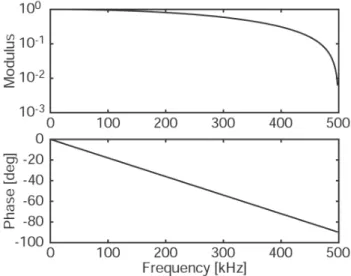
hard-Fig. 1.The upper panel shows the amplitude response of the digital filter and the lower panel portrays its phase response.
ware and our own hardware moves the 500-MHz frequency to zero, so that 500.25 MHz was shifted to 250 kHz and 499.75 MHz to−250 kHz. Continuous sampling was carried out at intervals of 1µs. The resulting data stream contains both frequency channels and, therefore, it is called multi-channel complex data.
Storing the signals has several benefits (Lehtinen et al., 2002); for example, the analysis can be done with quite flex-ible time and range resolutions, and Barker decoding with no sidebands can be carried out. Digital filters can be freely chosen, and the ground clutter can be eliminated in a better way than in the traditional ESR method. Since the transmit-ted pulses were also sampled, it is possible to investigate the phase behaviour of the transmission.
The analysis, including the channel separation, was done off-line. Channel separation was carried out by complex fre-quency mixing and consequent filtering. The multichannel complex data were multiplied by exp(−2π if0t ), where f0
is the mixing frequency (either 250 kHz or−250 kHz) and
t is the time. This operation downconverts the wanted fre-quency channel to zero and the unwanted frefre-quency channel to+500 kHz or−500 kHz. The unwanted high frequency channel is then filtered out by calculating a running mean over two samples. This corresponds to a low pass digital fil-ter shown in Fig. 1. The amplitude response in the top panel indicates that the unwanted high frequency signal at 500 kHz is sufficiently suppressed. The filter has a linear phase re-sponse, as seen in the bottom panel.
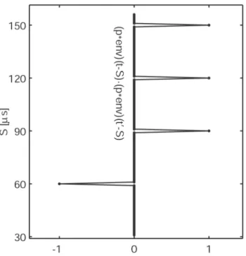
Fig. 2.The modulation envelope (env) of the Barker coded 5-bit code transmission and the decoded signal(p∗env). The bottom line of the sign pattern indicates the phases of the basic 5-bit modulation, the middle line the phases of the 5-bit Barker code and the top line the product of these two sign sequences, indicating the phase behaviour of the modulation envelope. The vertical dashed lines show the boundaries of the bits of the basic modulation.
from the second point. This decimation to a sample inter-val of 2µs corresponds to a 300-m step in range but, when the two lag profiles are combined, a 150-m range step is regained.
3 Range ambiguity of the measurement
In incoherent scatter experiments, one records the plasma autocorrelation function modified by the effects of both the modulation envelope and the impulse response of the re-ceiver. The concept of ambiguity functions was introduced to specify this kind of measurement (Woodman and Hag-fors, 1969). These functions depend in most general cases on both the range and lag variables. The range ambiguity function is the reduced form of the two-dimensional ambi-guity function which describes how one samples the iono-sphere. Mathematically, it can be written as (Lehtinen and Huuskonen, 1996)
Wt,t′(S)=(p∗env)(t−S)(p∗env)(t′−S), (1)
whereSis the total travel time of the transmitted pulse from the transmitter to a given point in the ionosphere and back to the receiver,pis the impulse response of the receiver, env is the modulation envelope,t andt′are two sampling times, and the overline indicates a complex conjugate.
The calculation of the range ambiguity functions for the 5-bit code is demonstrated in Figs. 2 and 3. An analogous calculation can be made for the 22-bit code. The top panel of Fig. 2 shows a measured modulation envelope of the Barker coded 5-bit phase code (env). The generation of this envelope from the combined basic code and Barker code is clarified by the bit patterns below the panel. The bottom line shows the bit pattern of the basic modulation, the middle line shows
the bit pattern of the Barker code and the top line show the combined modulation pattern obtained as a product of the two-sign sequences. Due to the 2-µs decimation, each 6-µs bit contains three data points. The thin vertical dashed lines indicate the boundaries of the bits of the basic modulation.
The bottom panel in Fig. 2 shows the result of Barker decoding, i.e. the function p ∗ env needed in calculating the range ambiguity function according to Eq. (1). The decoding is made in the manner described by Lehtinen et al. (2002). Unlike the conventional Barker decoding, this method produces no sidelobes. In principle, the impulse re-sponse of such a decoding filter has an infinite length, as al-ready pointed out by Sulzer (1989). The impulse response is not needed in practice, however. Using the line of thought presented by Lehtinen et al. (2002) the modulation envelope can be decoded according to the formula
(p∗env)(t )=F−1
F(env) F(b)
, (2)
whereFindicates Fourier transform and
b(t )=
nB−1 X
i=0
biδ(t−i1) (3)
is a digital Barker code ofnB bits with signs bi and a bit
length1. The result in the bottom panel of Fig. 2 shows no sidebands, but only short pulses in the beginning of the bits of the basic 5-bit modulation. The negative bit at the end produces a negative pulse. The pulses contain three sam-ple points, which means that the pulse length is equal to the Barker code bit length.
1432 B. Damtie et al.: High resolution observations of sporadic-E within the polar cap
Fig. 3.Calculation of the range ambiguity function of 30-µs lag for the 5-bit code. The left panel showsp∗env(t−S)and the middle panel
p∗env(t′−S), whent′−t=30µs. Their product, which is the range ambiguity function, is plotted in the right-hand panel.
is plotted assumingt = 150 µs and t′ = 180 µs, but any time values satisfying the conditiont′−t = 30µs would do, of course. The left-hand panel shows(p∗env)(150µs−
S)and the middle panel shows(p∗env)(180µs−S). The range ambiguity functionWt,t′(S), which is their product, is
plotted in the right-hand panel. It consists of four separate peaks, three positive and one negative. This means that the measurement of the first full lag contains information from four separate height ranges.
The other lags can be calculated in a similar way. The second and third full lags produce range ambiguities, but the range ambiguity function of the fourth full lag consists of a single peak. The treatment of the 22-bit code is analogous. The experiment also produces fractional lags (Huuskonen et al., 1996) which are obtained when values oft′−t are not multiples of 30µs.
4 Inversion and regularization
Both modulations in the experiment produce the first four full lags (30, 60, 90 and 120µs) and, in addition, the 22-bit code produces longer full lags at 30-µs intervals up to 21×30µs = 630µs. The range ambiguities associated with these lag profiles are removed by means of mathematical inversion. In addition, inversion also combines the same lag profiles from both modulations to produce single unambiguous lag profiles. Moreover, it is used to improve the statistics of the full lags by merging nearby fractional lags.
The inversion method is demonstrated here in terms of the 30-µs lag. Let us assume that we havenrange gates in the ionosphere. Due to the 1-µs sampling interval, the gate sep-aration is 150 m. These gates correspond tontravel timesSi,
i=1,2, . . . , n. Consequently, there are alsonunknown lag valuesxSi,i=1,2, . . . , n. They are collected into a column vector
x= xS1, xS2, xS3, . . . , xSn T
, (4)
where T denotes the transpose. The measured lag values from the 5-bit and 22-bit codes are collected into the vectors
m(5)=m(S5)
1, m
(5) S2, m
(5) S3, . . . , m
(5) Sn
T
(5) and
m(22)=m(S22)
1 , m
(22) S2 , m
(22) S3 , . . . , m
(22) Sn
T
, (6)
respectively. Here the subscripts denote the range gates of the topmost peak of the range ambiguity function. Correspond-ingly, the measurement errors are collected into respective vectors
ε(5)=ε(5)
S1, ε
(5) S2 , ε
(5) S3, . . . , ε
(5) Sn
T
(7) and
ε(22) =
εS(22)
1 , ε
(22) S2 , ε
(22) S3 , . . . , ε
(22) Sn
T
Fig. 4. The idealized range ambiguity function used in practice in defining the theory matrixAmfor the 30-µs lag.
The lowest gate (S1) is put at such a low altitude that the lag profile is practically zero at lower heights. This means that peaks of the range ambiguity function lying below the first gate give no contribution to the measurement.
Each measurementm(S5)
j orm
(22)
Sj is a linear combination of the unknown lag valuesxSi,i = 1,2, . . . , n, and the co-efficients in these combinations are determined by the corre-sponding range ambiguity functions. Figure 3 indicates that each main peak of the measured range ambiguity function has nearly equal magnitude, and between the peaks its value is zero. Therefore, in the analysis we assume equal peak heights and zero values between the peaks.
As an example, the coefficients of the linear combination between a single measurementm(1505) and the unknownsxSi,
i = 1,2, . . . , nare plotted in Fig. 4. It indicates that only
x150,x120,x90, andx60contribute tom(1505). There is no con-tribution from the rest of the unknowns. Hence, for all mea-surements of the 5-bit code, we can write a general equation
m(S5)
j = −xSj−90+xSj−60+xSj−30+xSj+ε
(5)
Sj. (9)
A similar analysis for a 22-bit code gives
m(S22)
j =xSj−600−xSj−570+. . . +xSj−30−xSj +ε
(22)
Sj . (10)
Here each subscriptSj −t indicates the travel time in
mi-croseconds for the respective range gate. It is also understood that, wheneverSj−t < S1, the value ofxSj−t is zero.
Equations (9) and (10) may be combined to obtain a matrix equation
m=Am·x+εm, (11)
where
m=
m(5) m(22)
(12) is the measurement vector,
εm= ε(5)
ε(22)
(13) is the error vector andAmis the theory matrix. Each row of
Amcontains the range ambiguity function of the
correspond-ing component of the measurement vector. In our simplified case it is a sequence of ones, minus ones and zeros, as indi-cated by Fig. 4. On each row ofAm, the same pattern appears
and it travels horizontally step by step with the row number. Hence, Am can be understood as a finite impulse response
(FIR) filter withxas an input.
The task is to find the best values of the unknowns when the measurements and their statistical error estimates are known. The unknownsx, the measurementsmand the true errorsεm are treated as random variables with appropriate probability densities. Ifxandmhave a joint probability den-sityD(x,m), the Bayes theorem for conditional probabilities gives
D(x,m)=D(x|m)D(m)=D(m|x)D(x), (14) where D(m)andD(x)are the probability densities of the measurements and the unknowns, respectively, andD(m|x)
andD(x|m)are their conditional densities.
The densityD(x)contains all information onxbefore the measurement. Hence, it is the a priori density ofx. We are interested in finding the conditional density of the unknowns after the measurement vector is known (i.e. the a posteriori distribution of x). Solving from Eq. (14), the a posteriori density is
D(x|m)= 1
D(m)D(x)D(m|x)
=C0(m)D(x)D(m|x). (15)
When the measurement is known,C0(m)is fixed and, there-fore, it is only a normalization constant. Also, when no a priori information is available, D(x)can be replaced by a constant.
At the moment of the measurement,xhas some unknown fixed value, and the error vector has some conditional density
Dεm(εm|x). Using Eq. (11), one can then show that
D(m|x)=Dεm(m−Am·x|x). (16) IfDεm(ε|x)is a Gaussian distribution with zero mean, insert-ing Eq. (16) in Eq. (15) and assuminsert-ing constantD(x)gives
D(x|m)∝Dεm(m−Am·x|x) ∝exp
−1
2(m−Am·x)
T ·6−1
m ·(m−Am·x)
, (17) where
6m= hεm·εT
1434 B. Damtie et al.: High resolution observations of sporadic-E within the polar cap
Fig. 5.The real part of the 30-µs lag of the autocorrelation function during four time intervals with a 150-m gate separation and a 10-s time resolution.
is the covariance matrix ofεm.
The maximum point of the a posteriori density in Eq. (17) is, in principle, the best value ofx. However, regularization is needed in order to obtain a stable solution. We do this by means of a statistical control of the lag value variation from gate to gate. More specifically, for eachi < n, we can write 0=xSi−xSi+1+ε
(i,i+1)
r , (19)
whereεr(i,i+1) is the change in the lag value from gateSi to
gateSi+1. In addition, we put the lag value to zero both on
the bottom and on the top of the profile, i.e. 0=xS1
(20) 0=xSn
All these equations can be combined into a single matrix equation
0=Ar·x+εr, (21)
where Ar is a (n+1)×nmatrix containing ones, minus
ones and zeros in appropriate places to satisfy Eqs. (19) and (20) for all values ofi. The values ofεr(i,i+1)and two zeros
corresponding to Eq. (20) are collected into a column vector εr, which will be treated as a(n+1)-dimensional Gaussian random variable with zero mean and a covariance matrix 6r = hεr·εT
ri. (22)
Equations (20) will be satisfied when the corresponding el-ements in the covariance matrix are put to zero. A diago-nal matrix is used and appropriate values are given to the variances allowing for sufficient changes in the lag profile from gate to gate. At altitudes where sporadic-E layers are observed, large values of the variances are used in order to match the steep gradients at the layer edges.
We can now combine Eqs. (11) and (21) into a single ma-trix equation
¯
m=A·x+ε, (23)
where
¯
m=
m
0
A=
Am
Ar
(24)
ε =
εm
εr
.
Then one can write an a posteriori densityD(x|m¯)analogous to that in Eq. (17), and the regularized solution is obtained by minimizing the quadratic form
q =(m¯ −A·x)T ·6−1·(m¯ −A·x). (25) The covariance matrix in this equation is
6= 6
m 0
0 6r
The most probable value ofx, resulting from a straightfor-ward calculation, is given by
ˆ
x=(ATm·6−m1·Am
+ATr ·6−r1·Ar)−1·ATm·6−m1·m. (27)
A formula for the statistical errors of the unknowns can also be derived.
This procedure is used to obtain unambiguous lag profiles for both full and fractional lags. In order to utilize the infor-mation from fractional lags, each full lag profile and some nearby fractional lags are then be combined to make a single profile. This is also carried out by means of mathematical inversion. The analysis will be explained in a separate work.
5 Results and discussion
The experiment was run at four separate time intervals on 16 November 1999. No software for importing lag estimates in the standard incoherent scatter analysis package is yet avail-able, and, therefore, the results are presented in terms of the lag estimates rather than plasma parameters.
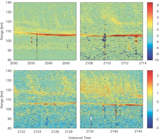
Figure 5 portrays the real part of the 30-µs lag of the au-tocorrelation function during the four time intervals 20:30– 20:48, 21:07–21:14, 21:21–21:19 and 21:33–21:46 UT. The results were obtained by using the 26-, 28-, 30-, 32- and
34-µs lag profiles in the inversion. The distinct vertical struc-tures in these plots are due to objects moving quickly through the radar beam or its sidelobes (satellites, meteors or space debris). This can be verified by plotting the data at extremely high temporal resolution, e.g. 0.008 s; then clear descending structures become visible. A simple way of cleaning the data from these echoes is to remove those profiles where they are present. It would be essential to do this before calculating the plasma parameters.
The most prominent features in these observations are sporadic-E layers with complex structures. In the beginning of the first time interval it actually consists of three sublayers, which cover a range of 108–115 km but descend with time and gradually merge into a thin single layer around 105 km. The layer thickness is of the order of 1–2 km. The layer is still strong during the second time interval and weaker but clearly visible during the other two intervals. In the last three panels the layer remains nearly at a fixed range of 105 km.
In addition, steeply descending, semiperiodic faint struc-tures are observed above the sporadic-E layers in the three first panels. In the fourth panel, a more continuous enhance-ment is visible which still may contain some periodicity. The period is of the order of 2–4 min, i.e. shorter than the Brunt-V¨ais¨al¨a period. Therefore, these structures cannot be attributed to acoustic gravity waves. During the first time interval, a band of enhanced structures is also visible at 90– 100 km.
Since the width of the incoherent scatter spectrum (for nearly identical electron and ion temperatures) is propor-tional to the ion-acoustic velocity
v+=p2kBTi/mi, (28)
Fig. 6. Real parts of plasma autocorrelation function at selected ranges from the time interval 20:30–20:48 UT.
the correlation length of the signal gives a rough view of the ratio Ti/mi. Here Ti and mi are the ion temperature
and mass, respectively, and kB is the Boltzmann constant.
A long correlation length indicates a smallTi/mi ratio and
vice versa. Figure 6 portrays the real part of the autocorre-lation function with error estimates at different ranges, from the whole observation period 20:30–20:48 UT. Within the sporadic-E layer, the first null lies at 300–360µs, while at 125 km it lies around 170µs. Although the difference in the correlation length may be partly due to the temperature gradient in the E-region, it cannot be explained in terms of the temperature only. Therefore, the conclusion is that the ion mass within the layer is greater than in the background E-region. This is in accordance with the sporadic-E theory which shows that thin layers can only be composed of long-lived metallic ions.
Estimates of the ion velocity can be obtained by assum-ing ionospheric plasma with symmetric power spectrum. If the observed autocorrelation function and the corresponding spectrum areR(τ )andS(ω), respectively, their relation is
S(ω)= Z ∞
−∞
R(τ )e−iωτdτ, (29) whereωis the angular frequency andτ is the lag. IfS(ω)
is symmetric aroundω0(i.e the Doppler shift isω0), a fre-quency shift
S(ω−ω0)= Z ∞
−∞
R(τ )e−i(ω−ω0)τdτ
= Z ∞
−∞
R(τ )eiω0τe−iωτdτ (30) makes the spectrum symmetric around zero frequency. Therefore,R(τ )exp(iω0τ )must be real. By putting its imag-inary part to zero, we obtain
1436 B. Damtie et al.: High resolution observations of sporadic-E within the polar cap
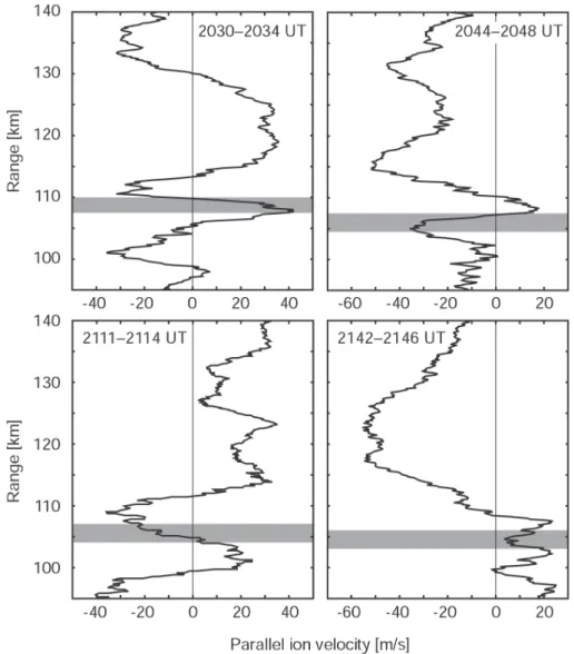
Fig. 7.Field-aligned ion velocity profiles at different time intervals. Positive velocity is upwards. The grey bands show the altitude of the sporadic E.
whereRrandRiare the real and imaginary parts of the
auto-correlation function. When the observed real and imaginary parts ofR(τ )are inserted in Eq. (31), together with the cor-responding lag valueτ, an estimate of the Doppler shift can be solved. Here positiveω0means motion towards the radar.
6 Interpretation of the layer observation
The classical explanation for the generation of sporadic-E is the wind shear theory (Whitehead, 1961; Axford, 1963; MacLeod, 1966; Chimonas and Axford, 1968), which was originally assumed to be effective at mid-latitudes only. Ac-cording to this theory, a sporadic-E observed at 105–110 km altitudes would be generated mainly by shears in the zonal neutral wind. The meridional neutral wind would become effective only at greater heights where the ion collision fre-quency is smaller than its angular gyrofrefre-quency.
Since the vertical ion velocity, due to horizontal neutral wind, is proportional to the cosine of the dip angle I, it has been argued that the wind shear mechanism is not ef-fective at high-latitudes where the dip angle is great. How-ever, sequential Es are regularly observed both in Sodankyl¨a (67◦22′N, 26◦38′E, cosI =0.23) and at the EISCAT site in Tromsø (69◦35′N, 19◦14′E, cosI =0.21). The sequen-tial Es are caused by shears in the S2 component of the at-mospheric tide, and, therefore, the wind shear mechanism is obviously effective at high-latitudes as well. At the ESR radar cosI =0.14, which means that vertical ion speeds at otherwise similar circumstances are reduced nearly to one-half of those at Tromsø or Sodankyl¨a. This would increase the time needed for compressing ions into a thin sheet, but could hardly prevent the layer generation.
vertical plasma compression creating the sporadic-E. This is not the case, however, and the reason is as follows. At E-region altitudes the ion velocity vector can be written as
v=ek·(E+u×B)+u, (32)
whereeis the positive elementary charge,kis the ion mobil-ity tensor,Eis the electric field,uis the neutral wind velocity, andBis the geomagnetic induction. Since, bothEandu×B
are perpendicular to B, this indicates that the field-aligned ion velocity is equal to the field-aligned component of the neutral wind velocity. Assuming horizontal neutral wind, the observed ion velocity is then equal to the field-aligned pro-jection of the meridional horizontal wind. Since, at these altitudes, the effect of the meridional neutral wind on verti-cal ion velocity is negligible in comparison with the effect of the zonal wind, the observed ion velocity does not give information on the vertical ion velocity profile.
Nevertheless, it is interesting to compare the field-aligned ion velocity profiles to the observed structures. The ion ve-locity was determined by calculating the Doppler shift from Eq. (31) separately for all 21 full lags and taking their aver-age. After converting the Doppler shift to velocity, the result-ing profile was smoothed by usresult-ing a 20-point runnresult-ing mean, which produced about a 3-km height integration. Field-aligned velocity profiles from four time intervals are plotted in Fig. 7. Here negative velocity is towards the radar and positive away from the radar. The grey bands indicate the altitudes of the sporadic-E during the same time intervals.
At 20:30–20:34 UT the layer is located just below 110 km in range. This is very close to a null in the field-aligned velocity at 110 km. The velocity is away from the radar below this null and towards the radar above. At 20:44– 20:48 UT the situation is different; a null lies again close to the layer height, but the field-aligned plasma velocity is directed away from it on both sides. Field-aligned plasma flow towards a null is again seen at 21:11–21:14 UT. Finally, at 21:42–21:46 UT the layer lies within a region of upward field-aligned velocity, but field-aligned flow towards a null is observed at a somewhat greater altitude.
Although the observed field-aligned ion velocity does not contain information on the vertical plasma velocity, it still re-veals the presence of shears in the meridional E-region neu-tral wind. This suggests that shears also exist in the zonal wind. Therefore, we can expect that the wind shear mecha-nism is active during the observation, but its role in the layer generation cannot be studied, since no measurements of the zonal wind are available.
The second possibility of explaining sporadic-E is the electric field mechanism (Nygr´en et al., 1984), which is pre-dicted to be most effective at high-latitudes, where strong electric fields are encountered. This theory leads to com-pressive vertical plasma flow if the ionospheric electric field points in some direction between west and north in the North-ern Hemisphere and between west and south in the South-ern Hemisphere. Even in this case the vertical ion veloc-ity is proportional to the cosine of the dip angle so that the same conclusions are valid as in the case of the wind shear
theory. Parkinson et al. (1998) have presented the number of observed sporadic-E layers versus electric field direction at Antarctica, showing convincingly that the electric field mechanism works at high-latitudes.
In order to find the role of the electric field in our case, data from the coherent SuperDARN radars (Greenwald et al., 1995) were investigated. The SuperDARN consist of radars both in Hankasalmi (Finland) and Pykkvibaer (Iceland), and their fields of view covers a wide region over the polar cap with Svalbard in the middle. During the observational period, both radars find coherent scatter with positive Doppler shifts above or close to Svalbard. This means that the plasma flow direction lies within the sector between west and south, indi-cating the presence of an electric field pointing in the sector between west and north. This field direction is in accordance with the electric field theory suggesting that the layer could be generated by the electric field mechanism.
7 Conclusion
We have shown structures of sporadic-E layers with a 150-m spatial resolution and a 10-s te150-mporal resolution within the polar cap ionosphere, using a new incoherent radar ex-periment. The range ambiguities produced by the experi-ment are removed by statistical inversion. The inversion so-lution is regularized by a method which is also explained. The layers have complex structures containing up to three sublayers with thicknesses of 1–2 km. They cover a height range of about 110–115 km, but then merge while descend-ing to 105 km. The layer remains visible for more than an hour. The plasma autocorrelation function is longer within the layer than in the surroundings, which is probably an in-dication of the presence of heavy metallic ions within the layer. Steeply descending, semiperiodic plasma structures above the sporadic-E layers are also observed.
Concerning the generation mechanism of the layer, two factors must be considered. For the first, the field-aligned ion velocity reveals the existence of wind shears at E-region alti-tudes, which suggests that shears also exist in the zonal wind and the wind shear mechanism is active. For the second, the ionospheric electric field points in the sector between west and north. This means that the electric field mechanism is also active. In this study, neither of the possible mechanisms can be excluded; they may be active simultaneously and their relative importance remains unknown.
1438 B. Damtie et al.: High resolution observations of sporadic-E within the polar cap ground clutter can be eliminated without affecting the
accu-racy of the measurements.
Acknowledgement. B. Damtie’s work was supported by Finnish
graduate school in Space Physics and Astronomy. The EISCAT measurements were made with special programme time granted to Finland. EISCAT is an International Association supported by Finland (SA), France (CNRS), the Federal Republic of Germany (MPG), Japan (NIPR), Norway (NFR), Sweden (NFR) and the United Kingdom (PPARC). CUTLASS is supported by the Parti-cle Physics and Astronomy Research Council, UK, the Swedish In-stitute for Space Physics, Uppsala, and the Finnish Meteorological Institute, Helsinki.
Topical Editor M. Lester thanks two referees for their help in evaluating this paper.
References
Axford, W. I.: The Formation and Vertical Movement of Dense Ion-ized Layers in the Ionosphere Due to Neutral WInd Shears, J. Geophys. Res., 68, 769–779, 1963.
Bristow, W. A. and Watkins, B. J.: Incoherent scatter observations of thin ionization layers at Sondrestrom, J. Atmos. Terr. Phys., 55, 873–894, 1993.
Bristow, W. A. and Watkins, B. J.: Effects of large-scale convection electric field structure on the formation of thin ionization layers at high latitudes, J. Atmos. Terr. Phys., 56, 401–416, 1994. Chimonas, G. and Axford, W. I.: Vertical Movement of
Temperate-Zone Sporadic E Layers, J. Geophys. Res., 73, 111–117, 1968. Greenwald, R. A., Baker, K. B., Dudeney, J. R., Pinnock, M., Jones,
T. B., Thomas, E. C., Villain, J.-P., Cerisier, J.-C., Senior, C., Hanuise, C., Hunsucker, R. D., Sofko, G., Koehler, J., Nielsen, E., Pellinen, R., Walker, A. D. M., Sato, N., and Yamagishi, H.: DARN/SuperDARN: a global view of the dynamics of high-latitude convection, Space Sci. Rev., 71, 761–796, 1995. Holt, J. M., Erickson, P. J., Gorczyca, A. M., and Grydeland, T.:
MIDAS-W: a workstation-based incoherent scatter radar data ac-quisition system, Ann. Geophysicae, 18, 1231–1241, 2000. Huuskonen, A., Nygr´en, T., Jalonen, L., Bjørn˚a, N., Hansen, T. L.,
and Brekke, A.: Ion Composition in Sporadic E layers Mea-sured by the EISCAT UHF Radar, J. Geophys. Res., 93, 603– 614, 1988.
Huuskonen, A., Lehtinen, M. S., and Pirttil¨a, J.: Fractional lags in alternating codes: Improving incoherent scatter measurements by using lag estimates at noninteger multiples of baud length, Radio Sci., 31, 245–261, 1996.
Kane, T. J., Gardner, C. S., Zhou, Q., Mathews, J. D., and Tep-ley, C. A.: Lidar, radar and airglow observations of a prominent Na/sporadic E layer event at Arecibo during AIDA-89, J. Atmos. Terr. Phys., 55, 499–512, 1993.
Kirkwood, S. and von Zahn, U.: On the role of auroral electric fields
in the formation of low altitude sporadic E and sudden sodium layers, J. Atmos. Terr. Phys., 53, 389–407, 1991.
Lehtinen, M. S., Markkanen, J., V¨a¨an¨anen, A., Huuskonen, A., Damtie, B., Nygr´en, T., and Rahkola, J.: A new technique in incoherent scatter experiments, Radio Sci., in press, 2002. Lehtinen, M. S. and Huuskonen, A.: General incoherent scatter
analysis and GUISDAP, J. Atmos. Terr. Phys., 58, 435–452, 1996.
Macleod, M. A.: Sporadic E theory. I. Collision-Geomagnetic Equi-librium, J. Atmos. Sci., 23, 96–109, 1966.
Mathews, J. D., Sulzer, M. P., and Perillat, P.: Aspects of layer electrodynamics inferred from high-resolution ISR observations of the 80–270 km ionosphere, Geophys. Res. Lett., 24, 1411– 1414, 1997.
Mathews, J. D.: Sporadic E: current views and recent progress, J. Atmos. Solar-Terr. Phys., 60, 413–435, 1998.
Miller, K. L. and Smith, L. G.: Reflection of radio waves by sporadic-E layers, J. Atmos. Terr. Phys., 39, 899–912, 1977. Miller, K. L. and Smith, L. G.: Incoherent Scatter Radar
Observa-tions of Irregular Structure in Mid-Latitude Sporadic E Layers, J. Geophys. Res., 83, 3761–3775, 1978.
Nygr´en, T., Jalonen, L., Oksman, J., and Turunen, T.: The role of electric field and neutral wind direction in the formation of spo-radic E-layers, J. Atmos. Terr. Phys., 46, 373–381, 1984. Parkinson, M. L., Dyson, P. L., Monselesan, D. P., and Morris, R. J.:
On the role of electric field direction in the formation of sporadic E-layers in the southern polar cap ionosphere, J. Atmos. Solar-Terr. Phys., 60, 471–491, 1998.
Smith, L. G. and Mechtly, E. A.: Rocket observations of sporadic-E layers, Radio Sci., 7, 367–376, 1972.
Smith, L. G. and Miller, K. L.: Sporadic-E layers and unstable wind shears, J. Atmos. Terr. Phys., 42, 45–50, 1980.
Sulzer, M. P.: Recent incoherent scatter techniques, Adv. Space Res., 9, (5)153–(5)162, 1989.
Wannberg, G., Wolf, I., Vanhainen, L.-G., Koskenniemi, K., R¨ottger, J., Postila, M., Markkanen, J., Jacobsen, R., Stenberg, A., Larsen, R., Eliassen, S., Heck, S., and Huuskonen, A.: The EISCAT Svalbard radar: A case study in modern incoherent scat-ter radar system design, Radio Sci., 32, 2283–2307, 1997. Whitehead, J. D.: The formation of sporadic-E layer in temperate
zones, J. Atmos. Terr. Phys., 20, 49–58, 1961.
Whitehead, J. D.: Production and prediction of sporadic E, Rev. Geophys., 8, 65–144, 1970.
Whitehead, J. D.: Recent work on mid-latitude and equatorial sporadic-E, J. Atmos. Terr. Phys., 51, 401–424, 1989.
Woodman, R. F. and Hagfors, T.: Methods for the measurement of vertical ionospheric motions near the magnetic equator by inco-herent scattering, J. Geophys. Res., 74, 1205–1212, 1969. Young, J. M., Johnson, C. Y., and Holmes, J. C.: Positive ion