Vol-7, Special Issue-Number2-April, 2016, pp886-900 http://www.bipublication.com
Research Article
Check the special moves Halftone a central sun sunspot different
angles using local correlation tracking
Monireh Askarikhah
ABSTRACT
Sunspots, solar magnetic field effect on a large scale are outstanding. In this research field study of surface movement (special move) in a Lightening Solar Shade Halftone sphere central angle of the sun in three different here. The evolution of current research and special horizontal movement in a sunspot on the basis of time-series observations imaging data in the blue spectral range with a wavelength continuum Central line spots active area of 4504 angstroms During the 3 day 10933NOAA dated 7 January (9.0) hours (UT) 12:35 until (UT) 12: 56, 8 January (8.0) hours (UT) 06: 00 to (UT) 06 21, Jan 9 (6/0) of the time (UT) 05: 00 to (UT) 05: 21, 2007 were obtained by using LCT (local correlation tracking) has studied. Halftone stains in the three-averaged (averaged over 10 consecutive images and averaged over 20 consecutive images) flow rate for each of the three categories Map angles (total 9 speed stream map) obtained, as well as a lot of speed graph speed on the map, each of which is for an angle we examined. What is clear in some parts of the maps quickly climb (eruption) in plasma and in some places fall (collapse) plasma-level Halftone be observed. The maps quickly, the (current) intensity Halftone patterns toward the inner penumbra shadow and movement patterns foreign to the outside strongly suggest Halftone That resulted in the dismissal of this shift is the dividing line that location is reached. Due to the frequency graph maps quickly we realized all three angles to this topic Slick passing moves quickly, especially given that the three angles of the half shadow has fallen. As well as speed of movement of the intensity of the Halftone patterns of the dividing line within the shadows of the reductions in external Halftone dividing line toward the photosphere increases.
Key words: special move, half shade, sun spots, magnetic field, the map quickly.
INTRODUCTION Halftone
Halftone probably a form of convection that in strong magnetic fields perpendicular to the surface at an angle of deviation from the big spots occur. Based on this issue, arguing that they are not exclusively a phenomenon of convection (5). Proper motion
To move the seeds of a half shadow of the so-called Proper Motion. In addition to the proper motion, intensity and longevity are three characteristics of the kinematic. . ProperMotionare not necessarily correspond to the actual movement of plasma. The characteristics of these movements may be regarded as a function of size, age,
evolution (young, old, and growing up, being decay and location) can-be (12).
.Ever shed flow
It is necessary to understand the nature of the fine structure half-shadow morphology of the velocity field and magnetic field break. The first attempt to measure the flow field by the British astronomer John Ever shedtook place in 1908 (4). The goal of this work was to test the theory of cyclone sunspot Hale (10).
Review the overall structure of sunspots
observation. Requires a fundamental observation is that sunspot model scales (location) was closely own again, and in terms of dynamic stability.. Modeling Halftone
Over the years, the dominant paradigm in the field of half-shadow based on flux tubes that are almost horizontal shaft parallel to the radial image and modeled and are placed in a more vertical magnetic field (11). Halftone a phenomenon complex interaction between magnetic convection and radiation at battles of the magnetic field oriented power (intensity) is average. A simple view on this issue is that the separation between the plume convection and magnetic makeup done, as in zero field gap model, to be considered. Embedded flux tube model (model not shoulder - irregular)
One of the models posed in recent research in the field of sunspots that is of particular importance, "Uncombed model" which the Solanki and in Montavon (1993) (14). It was suggested. They described a nearly horizontal flux tubes with a strong current parallel to the magnetic field can be circular polarization have seen That due to the lack of symmetries Stokes V is related to the formation, explains (11).
Flushing flow model
The first of the flux tube model proposed to explain Ever shedflows in Halftone flushing flow model proposed by Meyer and Schmidt (1968). In this model, there are differences in power between the two points of a flux tube to make a difference As a result, the gas pressure and flow in order to point the domain has the highest magnetic strength moves (11).
Moving flux tube model (dynamic)
These models are based on the assumption that half shadow fields by the level of predominantly horizontal flow near the surface were detected = 1. . The idea of magnetic flux tubes dynamics with the observational component of the magnetic Multiple in the penumbra is compatible.
Overshooting ovens – Magnetic
One of the interesting effects that can be studied with the drive tube is an ideal model for the Overshooting phenomenon is concerned. Shade sphere in terms of convective upward flow into the springs and bent by the magnetic forces along the pipe finds the horizontal direction.
Convective models: the zero gap rollers convective models
The concept of zero field in the gaps by Parker in 1979 (9) was introduced to show the spots shade, was developed by researchers such as Spruit and Sharmer 2006 (15) and serve to explain the bright filaments were half-shadow. They found that the formation of an embryo may... On the dark core disciplines as well which caused a small radiation field at the top of the gap is zero, produce.
Model convective rolls
Zero field gap model some similarities with the rollers (rolls) convective proposed by the philson, 1961. Here convection rollers are radially placed side by side... And two of these roller during rotation in the opposite direction to form and a rising flow in the central path and a stream down the side routes created (Figure 1).
Rapid structural changes Halftone
Figure 1.rapid transition irregular penumbra
Tracking Method
1. Local correlation tracking
Method "of local correlation tracking" to measure the velocity field, especially in a series of consecutive images of the penumbra spots (12) and also in granular tracking and tracing features various images visible spectrum with high angular resolution (1 13) used in the surface of the sun. 2-tracking feature
Sevioteka (12) changes when the core of the shadow of a sunspot fine structure in 1997, analysis and tracking of specifications for shadow spots on the application.Sevioteka and his colleagues used this method to measure the specific motion, brightness and longevity of seeds shadow in the penumbra of a sunspot half used. And later by Hamed loyal to identify the gaps and integrate tiny structures were correct in their lifetime (3). For further analysis, the following three fields (subset) of the sunspot penumbra shows that order-are selected. For grain separation under the half-shadow, a shadow mask geometry to remove bridges gaps optic selected by the minimum threshold of severity of clear specifications in the Iph8 / 0 and remove features, or photosphere photometric outside the boundary of the penumbra - the photosphere to be handled. After several preparatory phase segmentation method for separating seeds try to be half-shadow. . It is much more complicated than the case of moles shade and intensity of the penumbra is due to the complexity and rapid change. . An image differential (difference) by subtracting a smoothed image (window) of the original image calculated
from the difference image a mask binary (ones and zeros) with the peaks with larger quantities of a specified threshold as one and the rest are calculated as zero. This threshold varies for each image so that the values 06/0, 04/0, 03/0, respectively, in the mean (average quality) and worst picture (original) in the mask (zero and one) would be multiplied. The maximum intensity for each of beans seeds in half shadow place each time step (image) for wishes. Longevity of seed in half the number of images that are obtained shadow. Special time average speed of movement, with a least squares linear fit to place them in accordance with their position can be calculated. Special time average speed of movement, with a least squares linear fit to place them in accordance with their position can be calculated. In the last stage of data analysis along the grain of half-shadow conditions are met and the sub conditions are filtered to remove unknown structures (faults) in the track characteristics are investigated. . The method of tracking features by examining overlapping half-shade seed in the segmentation of consecutive images... And labeling them in any image as a semi-shade seed in two successive shots in there where. In this manner the time evolution of the physical characteristics of each grain consecutive images (at different times) record is saved (13).
Observational data Introducing data
basis of time-series images in wide continuum of blue spectral range with a wavelength of 4504 angstroms central line 10933NOAA active spots within 3 days in the seventh dated January (9.0) hours (UT) 12:35 until (UT) 12: 56, the eighth of January (8.0) hours (UT) 06: 00 to (UT) 06: 21, the ninth of January (6/0) of the time (UT) 05: 00 to (UT) 05: 21, 2007 were obtained by using LCT (local correlation tracking) we studied (in Central sun is the angle theta = cosѳ µ here.) 10933NOAA active spots within 3 days in the seventh dated January (9.0) hours (UT) 12:35 until (UT) 12: 56, the eighth of January (8.0) hours (UT) 06: 00 to (UT) 06: 21, the ninth of January (6/0) of the time (UT) 05: 00 to (UT) 05: 21, 2007 were obtained by using LCT (local correlation tracking) we studied (in here = cosѳ µ the central sun angle theta 10933NOAA active spots within 3 days in the seventh dated January (9.0) hours (UT) 12:35 until (UT) 12: 56, the eighth of January (8.0)
hours (UT) 06: 00 to (UT) 06: 21, the ninth of January (6/0) of the time (UT) 05: 00 to (UT) 05: 21, 2007 were obtained by using LCT (local correlation tracking) we studied ( here = cosѳ µ the central sun angle theta Astekle respectively s1, s2 and s3 are named. Pictures surveyed in each series includes 20 image burst immediately when time is 60 seconds.)By s1, s2 and s3 have been named. Pictures surveyed in each series includes 20 image burst immediately when time is 60 seconds.) Japanese satellite observational data Heynood recorded. A total of 60 pictures in your hands dimensions 380 × 690 370 × 755 homes for spots s1 and s2 home for spots and stains s3 is home to 420 × 650. The images are carefully aligned in the horizontal plane image and tandem arranged to fit into spots where false image on the page to be deleted. In Table (1) Details are
provided in the region.
Table 1. Sample spots at different angles Central Sun.
Average hours observing the coordinates on the page Sun ) Sun Watching ( Observation Date RegionNOAA active nam e 0/9 0/8 0/6 (404,-31) 12:35 – 12:56(UT)
06:00 -06:21(UT) (545,-35)
05:00 – 05:21(UT) (705,-45) 7 ﮫﯾﻮﻧاژ 2007 8 ﮫﯾﻮﻧاژ 2007 9 ﮫﯾﻮﻧاژ 2007 10933 10933 10933 S1 S2 S3 Data analysis
Halftone patterns in the intensity of sunspot track with the implementation of LCT
We LCT method utilizes a modified algorithm which flowmaker.pro program using the IDL programming language in 1994 by Horace Molon (6) wrote his senior thesis... By using new parameters in accordance with the observations of the sunspot 10933 NOAA run on three consecutive days And to calculate the velocity fields, especially the penumbra of the 20-minute set of images for each day of the seventh (9.0), eighth (8.0) and ninth (6/0) in January 2007 described above.
Determine the tracking parameters
can take LCT used to find the horizontal velocity field.
Steps to create fast map
The study sunspot sample in this study included a range of different situations heliocentric solar disk over three consecutive days. . According to the table (1) away from the center of the solar disk, the special measure is actually true horizontal velocity plotted sunspot on the surface perpendicular to the surface of the field of view (LOS) are. . LCT method with the help of function and weight change tracking parameters (by trial and error and future considerations original images obtained) To the best maps on the number of consecutive images appear sharp averaged... And springs and wells and the dividing line in the half shadow or penumbra time evolution movement patterns on the surface of the track. Surface velocity field for the detection of penumbra and statistical comparison should Halftone spots of shade and shade area surrounding sphere separated by determining the intensity threshold. . The entire process of creating the mask and apply it on the Halftone for a time
series on the panel of Figure 2 is depicted and is made up of the following:
A)The field of view that we want to analyze it (the department arc second spatial scale are used.)
B)Structures using the methodology of calculation of the special moves LCT and map the flow for the entire field of view in the grain structure for each image time series over three consecutive days in three different central angle of the sun.
C)Create a binary mask for sunspots (the penumbra) via highly configurable thresholds so that the lowest amount that we consider the intensity level and the highest amount of intensity shade shadow sphere less. As a result of a binary mask in which all parts of the penumbra at number one and the rest of the image are marked with zero build.
D)Apply the mask made on the flow field. E) Open sharply drawn amounts. Values that have
been re-drawing are shown with gray scale, bright or dark areas correspond to large and small velocity.
(b) (A)
(d) (C)
(e)
Figure 2.Business process steps taken to produce the map. A) field of view for analysis. B) the current map. C)
RESULTS
Statues map sunspot penumbra surface
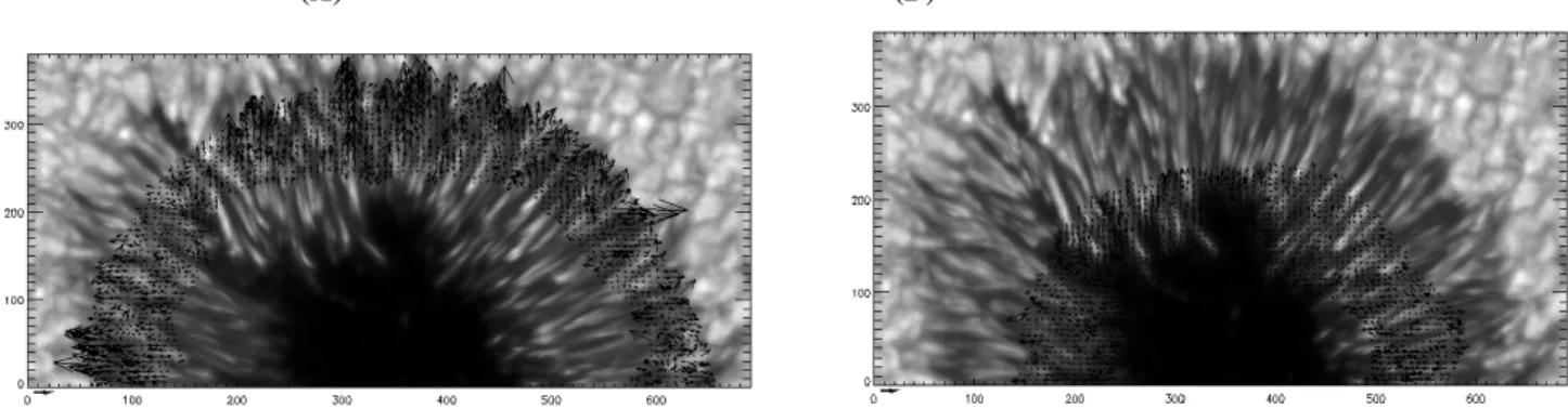
In this study, we each series of 20 consecutive images immediately angles that time is one minute to two subsidiaries: 10 minutes from one to 10 and 11 to 20 as well as the entire series (20 images) divide And for each of the series of images to obtain an average velocity map that eventually reached three series speed map for each of angles. A total of 9 Halftone sunspot surface velocity maps in three different angles over three days will bring. . LCT algorithm house to house in the consecutive images (in this study, the distance of an image of the) local solidarity and calculate the intensity for every point rate gains. Figures 3 (a) averaged over 10 maps the first image and the second image (b) and (c) averaged over 10 consecutive averaged over the entire 20 Image 9/0 = Figure 4a averaged 10 the first image and the second image (B) and (C) averaged 10 to 20 consecutive images at 8/0 =, Figure 7 (a) averaged over 10 the first image, the second image and averaged 10 c averaged over 20 consecutive images in 6/0 = shown, In the lower left corner of the thick black horizontal line, the speed of one kilometer per second. In most of the images obtained with less than a kilometer per second speed The speed of this amount is also shown in
Fig. Also seen in the map by sharply at a certain radial distance, velocity vectors into the shade for some and for others out towards the penumbra (the photosphere). Following this shift comes in the form of the dividing line,this is shown in Figure 3, which is the first day of the first series. The boundary between the inward and outward movement of the LCT locus of points defined zero speed is almost in the middle of the penumbra. It is important to know what speed obtained from the study of maps comes the velocity vectors near the outer edge of the other parts are bigger Halftone... That is the fact that half intensity pattern on the outer edge of the penumbra shadow move faster. The severity of half-shadow patterns on the outer edge of the penumbra faster they move. The velocity vectors in the inner edge of the penumbra, the shadow near the smaller figures show... And in some parts of the penumbra can be seen that speed and intensity patterns also tend to zero. Following the eruption and collapse the plasma source with velocity vectors, respectively divergent and Well with the flow velocity vectors converging on the map as a result convective flows of plasma and magnetic field interaction is penumbra That mass and energy are directed to the spots, are determined. In Figure 5 wells and springs with oval corrugated represented.\
Figure 3. Black Halftone line into two parts move inward and outward movement of division that defined the dividing
Figure 4. Map of the horizontal velocity field for the image to 10: 9/0 = the oval shape well, convergent velocity
vector (collapse) and diamond Fountains, divergent velocity vector (eruption) shows.
(a)
(b)
(c)
Figure 5. The horizontal field map statues to images of a) 10 b) 11 to 20 C) one to twenty angles 9/0 ==
(a) (b)(C)
(a) (b)
( c)
7. Map the horizontal speeds for image alpha) of one to 10 b) 11 to 20 C) up to 20 angles 6/0=
Now we want to have a map of speed derived from techniques LCT frequency graph for each of the time series of angles 9 = 0/8/0 = 6/0 = to draw respectively in Figures 8 and 9 and 10 are displayed.
(a)
(b)
(c )
(b) (a)
(c)
Figure 9 frequency charts for velocity maps a) 10 b) 11 to 20 c) a 20 angle (8.0) (A)
(B)
(C )
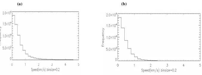
As is clear from the chart lot of speed, a smaller speed of m / s 500 most rapidly are abundant. Table 2% less than homes that speed m / s 500 have been brought for all divisions.
Table 2 shows the percentage of homes that LCT rate of less than 500 meters per second.
The percentage of homes that are faster than 500 meters per second .
700 Pictures of one to 10
) 9 / ٠ =
( 700 Pictures 11 to 20) 9 / ٠ =
( 700 Pictures of one to 20) 9 / ٠ =
( 800 Pictures of one to 10) 8 / ٠ =
( 800 Pictures 11 to 20) 8 / ٠ =
( 500 Pictures of one to 20) 8 / ٠ =
( 800 Pictures of one to 10) 6 / ٠ =
( 600 Pictures 11 to 20) 6 / ٠ =
( 500 Pictures of one to 20) 6 / ٠ =
(According to the map of the speed and frequency graph obtained... To averaged 10 and 20 consecutive images to the conclusion That the average speeds measured on 20 consecutive images is far smaller than the average of the 10 consecutive images.
3-2-5-study comparing changes each time series at a frequency graph
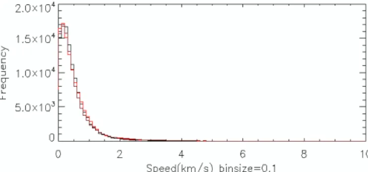
To further explore the changes in the graph of all three series when a given angle of incidence we plotted on a graph And it was observed that the frequency of each series of charts given time will not change much; But as seen in Figure 9 is an abundance graph from 0 to 19 (the whole series) each of the angles plotted. Black high-frequency line graph related to 9/0 =
، red solid line 8/0 =
، and gray solid line / 6
،= 0. . According to Chart 12, we see horizontal velocity for movement in a given spot angles larger central sun rises.Figure 11. Prevalence of the series when all three angles in a chart (black solid line graph of the frequency = 0/9,
full line of red 8/0 = and gray solid line 6/0 = )
(a)
(b)
(c)
Figure 12. The dividing line velocity field for a) 9/0 ==٠
A, B) 8/0 ==٠
, c) 6/0 ==٠
(a)(b)
Figure 13. Map statues horizontal field angle the entire time series (9/0 =
() to image a) external Halftone b)foreign Halftone
(A) (B)
Figure 15. Map statues horizontal field angle the entire time series (6/0 =
) to image a) external Halftone b) internalHalftone
(a) (b)
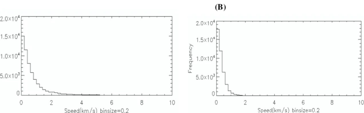
Figure 16. Frequency distribution of horizontal velocity map of the entire series when the angle (9/0 =
() to imagea) external Halftone b) internal Halftone
(A) (B)
Figure 17. Frequency distribution of horizontal velocity map of the entire series when the angle (8/0 =
) to image a)(A)
(B)
Figure 18.Frequency distribution of horizontal velocity map of the entire series when the angle (6/0 =) to
image a) external Halftone b) internal Halftone By comparing the frequency graph horizontal velocity maps of the penumbra, the outer and inner penumbra, we realize Halftone outside of the dividing line in the photosphere increases. Figure 19 Horizontal Frequency strong Maps and Halftone inner outer black color is red entire series when all three angles is depicted in a graph, chart A) 9/0 = A, B) 8/0 =, c) 6/0 = shows. As we part.
(A) (B)
(C)
Figure 19. Prevalence of horizontal velocity map of the entire series Halftone Black exterior and red interior Halftone
(A) (B)
(c )
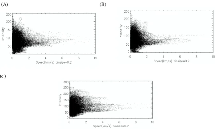
Figure 20. Correlation between intensity and size charts sharply over the half shadow of one to 20, A) 9/0 =
b) 8/0=
C) 6/0 =
The figure measures the correlation between the intensity of the penumbra and sharp intensity patterns each time series comes... Great intensity is related to the average velocity and a certain correlation between these two parameters is seen.
CONCLUSION
The present study examines the evolution and current special horizontal movement in a sunspot on the basis of time-series observations... Imaging data in spectral range with a wavelength in the blue spectrum centerline 4504 Å of the active region 10933NOAA spots during 3 days in May and January 7 (9.0) of the hours (UT) 12:35 until (UT) 12: 56, 8 January (8.0) hours (UT) 06: 00 to (UT) 06: 21, 9 January (6/0) of the time (UT) 05: 00 to (UT) 05: 21, 2007 obtained the using LCT (local correlation tracking) there. The results of the correlation tracking method is applied topically on the 10933 NOAA sunspot penumbra can be summarized as follows.
(1) The track, intensity patterns and sharply less than 500 meters per second is very high, so that the image is averaged over twenty
consecutive averages sharply lower intensity patterns of 500 meters per second.
(2) 2-What is clear in some parts of the maps quickly climb (eruption) in plasma and in some places fall (collapse) plasma can be seen in the penumbra.
(3) .According to the plans to move quickly found that brilliant features built into the shade and semi-shade the direction of the brilliant features of foreign penumbra is the outer boundary of the penumbra.
(5) Due to the frequency graph maps quickly we realized all three angles to this topic Slick passing moves quickly, especially given that the three angles of the half shadow has fallen.
(6) Special radial movements tend to move in the penumbra inner and outer tend to be outside in the penumbra.
(7) Spank intensity patterns in the inner penumbra of the shadow line dividing the lower and outer penumbra of the dividing line in the photosphere increases...
REFERENCES
[1] Ambroz, P., Sol. Phys., 198, 253, (2001) [2] Haimin, W., Deng, N., Chang, L., APJ,
Astro-ph. SR (2012)
[3]Hamedivafa, H., Solar phys, 270, 75, (2011) [4] Jahn, K. 1992, in ASP Conf. ser. 118, ed. B.
Schmieder, J. C. del Toro Iniesta, & M. Vazquez, 122
[5] Marquez, I., Sanchez Almeida, J &J.A.Bonet. The AstroohysicalJornal, (2006)
[6] MolownyHoras, R., & Yi, Z., Internal Report No. 31, Institute of Theoretical Astrophysics, University of Oslo
[7] November, L. J., APPL. Opt., 25, 392, (1986) [8] November, L. J., Simon, G.W., APJ, 333,
427, (1988)
[9] Parker, E. (1979). APJ, 230, 905.
[10]Remple, Living Reviews in solar physics, Irsp- (2011)
[11]Sharmer, G., Space sci Rev, (2009)
[12]Sobotka, M., V_azquez, M., Bonet, J.A., Hanslmeier, A., &Hirzberger, J., APJ, 511, 436, (1999)
[13]Sobotka, M., Brandt, P. N., & Simon, G. W., A&A, 328, 689, (1997)
[14]Solanki, S., Montavon, C., A&A, 275, 283-292, (1993)
[15]Spruit, H., &Scharmer, G., A&A, 447, 343-354, (2006)