www.atmos-chem-phys.net/14/3065/2014/ doi:10.5194/acp-14-3065-2014
© Author(s) 2014. CC Attribution 3.0 License.
Atmospheric
Chemistry
and Physics
Interaction between dynamics and thermodynamics during tropical
cyclogenesis
S. Gjorgjievska and D. J. Raymond
Physics Department and Geophysical Research Center, New Mexico Institute of Mining and Technology, Socorro, New Mexico 87801, USA
Correspondence to:S. Gjorgjievska ([email protected])
Received: 26 April 2013 – Published in Atmos. Chem. Phys. Discuss.: 16 July 2013 Revised: 25 January 2014 – Accepted: 17 February 2014 – Published: 27 March 2014
Abstract. Observational data of tropical disturbances are analyzed in order to investigate tropical cyclogenesis. Data from 37 cases observed during three field campaigns are used to investigate possible correlations between various dynamic and thermodynamic variables. The results show that a strong mid-level vortex is necessary to promote spin up of the low-level vortex in a tropical cyclone. This paper presents a the-ory on the mechanism of this process. The mid-level vortex creates a thermodynamic environment conducive to convec-tion with a more bottom-heavy mass flux profile that exhibits a strong positive vertical gradient in a shallow layer near the surface. Mass continuity then implies that the strongest hor-izontal mass and vorticity convergence occurs near the sur-face. This results in low-level vortex intensification.
For two of the disturbances that were observed during sev-eral consecutive days, evolution of the dynamics and ther-modynamics is documented. One of these disturbances, Karl, was observed in the period before it intensified into a tropical storm; the other one, Gaston, was observed after it unexpect-edly decayed from a tropical storm to a tropical disturbance. A hypothesis on its decay is presented.
1 Introduction
The genesis phase is the least understood part of the tropical cyclone life cycle. In this paper we use the term cyclogen-esis to refer to the intensification of a precursor disturbance into a tropical storm (TS). We know that tropical storms de-velop from preexisting finite amplitude disturbances, such as mesoscale convective systems (MCSs) that exhibit cyclonic vertical vorticity. They often form within monsoon troughs
or tropical waves. Genesis involves processes that are much less important during the mature phase of a tropical cyclone. Favorable conditions for these MCSs to develop into tropi-cal storms are high sea surface temperature and low vertitropi-cal wind shear. These conditions are probably best summarized by Gray (1968). Although during a hurricane season many MCSs develop, only a small percentage of these turn into tropical storms, even in favorable environmental conditions. How are the developing disturbances different from the non-developing? McBride and Zehr (1981) compared composites of non-developing and developing cloud clusters. Their main findings were as follows: both systems have warm cores in the upper levels, but the warming is more pronounced in the developing clusters; the static stability is somewhat smaller for the developing systems; the developing composites ex-hibit less vertical wind shear near the system center, but there is a requirement for a certain kind of wind shear surrounding the developing system; and the developing clusters exhibit larger positive vorticity at low levels.
thermal wind balance, the precursor mid-level vortex corre-sponds to a cold-core vortex below the vorticity maximum and warm-core vortex aloft. Later the near-surface vortic-ity increases, a warm-core vortex develops in the lower tro-posphere, and genesis occurs. The available observations, though not abundant, show support for this pathway of devel-opment. This was the case with typhoon Robyn (1993) (Harr and Elsberry, 1996) and typhoon Nuri (2008) (Raymond and López, 2011) in the west Pacific and hurricane Guillermo (1991) in the east Pacific (Bister and Emanuel, 1997). There is also evidence of the pre-hurricane Dolly (1996) in the At-lantic developing a mid-level vortex 35 h before it was up-graded to a tropical depression (TD) (Reasor et al., 2005). This pathway of development was also observed in numerical simulations. Nolan (2007) used a model to simulate develop-ment of tropical cyclones, initiating each simulation with a preexisting vortex. All of his simulations, even the ones initi-ated with a low-level vortex, first developed a mid-level vor-tex before low-level spin up occurred. A “top-down” devel-opment, meaning a mid-level vortex developed as a precursor to cyclogenesis, was evident in these studies, but there was no physical explanation given of how the mid-level vortex en-courages vorticity intensification near the surface. Later Ray-mond et al. (2011), based on the previous theoretical work by Raymond and Sessions (2007), hereafter RS07, and some ob-servations, suggested that the thermodynamic state of the at-mosphere within the mid-level vortex favors convection that aids the formation of the low-level vortex.
Meanwhile, Dunkerton et al. (2009) hypothesized that genesis is initiated within westward moving tropical waves, in a region near the intersection of the wave axis and the crit-ical latitude. The latter is defined as the latitude at which the wave speed is the same as the background flow. They call this intersection a sweet spot, and the broader recirculat-ing area around it is dubbed the pouch. The pouch exhibits low-level cyclonic vorticity and minimal strain rate. The air within the pouch is protected from lateral dry air intrusion, and thus continuous moist convection is enabled, which fur-ther increases the cyclonic vorticity. Ultimately, the wave– convection interaction leads to the development of rotating deep convection. Aggregation of low-level vorticity associ-ated with the rotating deep convection results in a vortex in-tensification in the lower troposphere and, subsequently, in the middle and upper troposphere. The vortex eventually sep-arates from the mother wave. This hypothesis, known as the marsupial paradigm, represents so-called “bottom-up” devel-opment.
The terms “top-down” and “bottom-up” give the impres-sion of two opposed theories. Wang (2012) conducted nu-merical simulations of hurricane Felix (2007) and analyzed the genesis on two different scales, 2×2 degree box (meso-beta) and 6×6 degree box (meso-alpha), both centered on the pouch at 850 hPa. Her results show a “bottom-up” path-way of development on meso-beta scale, and a “top-down” pathway of development on meso-alpha scale. Dunkerton et
al. (2009) also noted that the upward and downward path-ways are not mutually exclusive and may co-exist on dif-ferent scales. We believe that both the mid-level vortex (at meso-alpha) and the pouch (at meso-beta) are important for tropical cyclogenesis and they are perhaps two pieces of the same puzzle. In the future we should avoid the terms “top-down” and “bottom-up”, as they are relative and are a source of confusion.
In the present paper we analyze data from developing and non-developing disturbances that were observed during the 2010 hurricane season in the tropical Atlantic and the Caribbean. For part of the analysis we also use data gathered in the west Pacific during the 2008 typhoon season. The re-sults reinforce the importance of the mid-level vortex as a precursor to tropical storm formation.
There are two purposes to this paper. First, we present a theory on the mechanisms by which the mid-level vortex fos-ters low-level vortex spin up. Second, we hypothesize as to how an observed storm decayed. The remainder of this pa-per is organized as follows. The second section of this papa-per describes the data and the methods that are used to analyze the data. Section 3 gives the equations we use for our cal-culations. In Sect. 4 we give background on the theory. The results from our analysis are presented in Sect. 5. We discuss the results and give concluding notes in Sect. 6.
2 Data and methods
The second data set is from the NASA field campaign Genesis and Rapid Intensification Processes (GRIP), for which the time period and target area overlapped with PREDICT. The experiments were coordinated, and for sev-eral pre-storm disturbances observations were done by both GRIP and PREDICT. In the present study we use dropsonde data from six GRIP missions, for which dropsondes were launched from the NASA DC-8 aircraft. Braun et al. (2012) describe the tools and the objectives of the GRIP experiment. The third data set was gathered during the field campaign Tropical Cyclone Structure (TCS08) experiment that took place in the period August–September 2008. The Naval search Laboratory (NRL) P-3 aircraft and two Air Force Re-serve WC-130 aircraft deployed dropsondes over the west Pacific. In addition, the P-3 aircraft took wind measurements using the ELectra DOppler RAdar (ELDORA). The qual-ity control on the dropsonde data was also done by EOL. See Raymond and López (2011) and Raymond et al. (2011), hereafter RSL11, for more information.
Dropsondes measure temperature, pressure, horizontal wind and relative humidity continuously as they descend, so that the vertical resolution of the collected data is good. However, the horizontal resolution is coarse (∼1◦×1◦). We further use a three-dimensional variational (3-D-Var) anal-ysis to obtain values of the meteorological parameters in the entire observational volume. For each mission we first vertically interpolate the data from each dropsonde, so that they all have the same vertical interval and step size. We then also calculate the mixing ratio, moist entropy, satura-tion mixing ratio, and saturasatura-tion moist entropy at every grid point. The dropsondes are not launched at the same time but rather one at a time, roughly one dropsonde every 7– 10 min. Depending on the size of the disturbance, it takes 2–4 h for all the dropsondes to be released. For the purpose of our analyses we adjust dropsonde positions in the moving frame of the disturbance to their locations at a standard ref-erence time. The moving frame is defined as a frame moving with the propagation velocity of the disturbance. The prop-agation velocity is calculated from the final analysis (FNL) for the Global Forecasting System by tracking the vorticity center averaged between 850–700 hPa. The standard refer-ence time is usually chosen to be roughly half way through the period of dropsonde deployment, resulting in a snapshot of the disturbance at this time. The snapshot assumption is adequate for studying mesoscale processes. Then we spec-ify a three-dimensional grid, moving with the observed dis-turbance, with longitude–latitude resolution 0.125◦×0.125◦ and vertical resolution of 0.625 km. The dropsonde data are assigned to appropriate grid points. The data are then interpo-lated to the full grid using the 3-D-Var scheme. The vertical velocity is calculated by strongly enforcing mass continuity in the 3-D-Var scheme. The 3-D-Var analysis also imposes a certain degree of smoothing in order to remove noise and aliasing. Finally, we mask the file in order to consider only
the area covered by the dropsondes. The 3-D file at this point is ready for analysis.
A detailed description of the 3-D-Var technique used in the present work is given by López and Raymond (2011) and Raymond and López (2011). The values of the 3-D-Var pa-rameters used here are the same as in RSL11.
3 Equations
3.1 Vorticity budget equation
We adopt the flux form of the vorticity budget equation from Raymond and López (2011):
∂ζz
∂t = −∇h·(ζzvh−ζhvz+ ˆk×F)−kˆ· ∇hθ× ∇h5. (1) Here,v=(vh, vz)is the storm-relative velocity,ζ=(ζh, ζz)
is the absolute vorticity,F is a force due to surface friction, θis the potential temperature, andkˆis the unit vector in the vertical direction. The quantity 5=Cp(p/pref)R/Cp is the
Exner function, whereCpis the specific heat at constant
pres-sure,Ris the gas constant for dry air andpref=1000 hPa is
a constant reference pressure. The subscriptshandzdenote the horizontal and vertical components, respectively. The last term on the right hand side represents the vertical component of the baroclinic generation of vorticity. For environments that are characterized by weak baroclinicity, as in the tropics, this term is insignificant and thus can be neglected. The ex-pression in parentheses is the horizontal flux ofζz: the first
term represents the flux due to advection, the second is the flux due to tilting, and the third is the flux due to the frictional force. The frictional force per unit mass,F, is estimated by F=τexp(−z/zs)
ρzs
, (2)
wherezis the height,zs is a scale height which represents
the average depth of the boundary layer, and
τ= −ρblCD|Ubl|Ubl (3)
is the surface stress. The symbolρrepresents the density,Ubl
is the horizontal wind, andCDis a drag coefficient, which we
calculate using the bulk formula
CD=(1+0.028|Ubl|)×10−3. (4)
HereUbl has units of meters per second. This is the same
formula for the drag coefficient as used in RSL11. 3.1.1 Thermodynamic variables
by the vertically integrated saturated precipitable water,
SF= Rh
0ρrdz
Rh
0 ρr∗dz
, (5)
wherer∗is the saturation mixing ratio.his the height of the domain. Bretherton et al. (2004) found that this parameter controls most of the variability in rainfall over the tropical oceans. The instability index is a measure of the tropospheric instability to moist convection and it is defined as
1s∗=slow∗ −shigh∗ . (6)
Hereslow∗ is the saturated moist entropy averaged over the layer between 1 and 3 km andshigh∗ is the saturated moist en-tropy averaged over the layer between 5 and 7 km. As the saturated moist entropy is a proxy for temperature at a fixed pressure level, larger values of this parameter are associated with an atmosphere more unstable to moist convection.
4 Background
It has long been known that both dynamics and thermody-namics are involved in the process of tropical storm forma-tion. Dynamics can affect the thermodynamic processes and vice versa, so there is feedback between the two. Hence, in order to understand tropical cyclogenesis one should not only understand both the dynamics and thermodynamics, but should also understand how they work together and how they interact constructively to create a tropical storm. Observa-tions of pre-storm disturbances over the last two decades have revealed that a mid-level vortex forms prior to trop-ical storm genesis. A low-level mesoscale vortex may or may not exist prior to a mesoscale mid-level vortex devel-opment, however, development/intensification of a low-level cyclonic vortex into a TS follows after an establishment of a mesoscale mid-level vortex. The Haynes and McIntyre (1987) flux form of the the vertical vorticity equation does not recognize direct communication between vortices at dif-ferent levels, as it considers the dynamics alone. The theory we present here explains how the mid-level vortex influences the low-level vortex by changing the thermodynamic strati-fication of the troposphere. In thermal wind balance, a mid-level vortex is associated with a cold-core vortex below it and with a warm-core vortex above it.
To test the effect of the temperature perturbations associ-ated with a mid-level vortex, RS07 did an experiment using a cumulus ensemble numerical model. The model was non-rotational, with interactive radiation. The simulations were done on a two-dimensional domain. First, they ran the model to radiative-moist-convective equilibrium (RCE). Then they used the RCE vertical profile of potential temperature and the corresponding vertical profile of moisture as reference pro-files for weak temperature gradient (WTG) simulations. Two
sets of WTG simulations were done. One with perturbed tem-perature profile, while the moisture profile remained unal-tered, and another set with perturbed moisture profile, while the temperature profile remained the same. Control runs were done with unchanged reference profiles. The experiments re-garding added moisture to the numerical troposphere with unaltered stability to moist convection resulted in more rain-fall per unit surface entropy flux, while the resulting vertical mass flux profiles did not change their shape with respect to the control run. They only increased in magnitude. The other set of experiments, with unaltered moisture but changed sta-bility to moist convection behaved differently. Stabilization of the troposphere (negative potential temperature perturba-tions applied below 5 km and positive perturbaperturba-tions above 5 km) resulted in increased rainfall, but it also produced a differently shaped vertical mass flux profile from the con-trol run. Its maximum occurred at a lower elevation (more bottom-heavy mass flux) and it had a larger magnitude. In other words, it exhibited a strong positive vertical gradient in a shallower layer near the surface. Such a mass flux would produce more low-level vorticity convergence and conse-quently low-level spin up. Raymond et al. (2011) analyzed observational data of seven tropical disturbances and found support for the theoretical results of RS07.
Raymond and Sessions (2007) did not discuss the mech-anisms by which a more stable troposphere produces a stronger and more bottom-heavy mass flux profile. We did additional diagnostics of their simulations and found that the parcel buoyancy and the surface entropy fluxes are re-sponsible for the observed changes in the mass flux profile. These are affected by the applied temperature perturbations (cooling below 5 km and warming above 5 km) in the fol-lowing way. The parcel buoyancy above∼2 km is reduced, with larger reductions occurring at higher elevations. Con-sequently, the parcels encounter the level of neutral buoy-ancy at a lower elevation. The parcel buoybuoy-ancy below 2 km is slightly increased, which corresponds to smaller convective inhibition (CIN). The surface entropy fluxes are larger in the perturbed cases, as a result of the lowered atmospheric tem-perature near the sea surface. We conclude that a more sta-ble troposphere produces a more bottom-heavy vertical mass flux profile as a result of the corresponding changes in the parcel buoyancy. The larger mass flux magnitude is fostered by the larger surface entropy fluxes.
a timescale of 3.5 h. Wissmeier and Smith (2011) did a study on this subject. They conducted idealized numerical exper-iments, to explore the effects of ambient vertical vorticity on convective updrafts, focusing on convection that devel-ops within tropical depressions and pre-depressions. For the types of rotation they studied, they did not find the rotation to have large effects on the updraft dynamics. Therefore, we believe that introducing rotation would not change the results enough to affect the conclusions of the current work.
5 Results
The results are divided into two parts. The first part employs the 7 observational cases from Raymond et al. (2011) and 30 additional cases from PREDICT and GRIP, to further ex-plore possible correlations between dynamic and thermody-namic variables. The second part presents the evolution of two disturbances that were observed during PREDICT and compares the two. One of those, Gaston, had a tropical storm status for a few hours only, after which it started to decay. Nevertheless, it was observed over the course of the next 5 days, as it was expected to intensify again. However, it kept decaying slowly until it dissipated and we take it as a decaying/non-developing case. The other is Karl, a develop-ing system that eventually became a major hurricane. It was observed extensively in its pre-storm phase.
Many of the results shown in this paper are obtained by horizontal averaging over an area for each disturbance. A valid question arises here, regarding the proper area to be considered for analysis. Unfortunately, there does not yet ex-ist an established, objective method for quantitatively com-paring the observed disturbances. It is difficult to find such a method, because of inconsistencies among disturbances. There are two main factors driving these inconsistencies. First, there are differences in aircraft data sampling. The ob-servational areas have different sizes and shapes, and the circulation centers are in different locations within the ob-servational area. The other source of inconsistency which is probably more important but is often neglected, is the uniqueness of each disturbance, regardless of the data sam-pling area. No two disturbances have the same size, shape, and structure, nor do they occur within identical environ-ments. The pre-storm disturbances in particular are highly non-axisymmetric. Therefore, whatever method is chosen to select an area for analysis will skew the results in some way. For example, one may choose a circular or a rectangular area centered on a circulation center at a certain level for all the disturbances. The size of the area may cover 50 % of the ac-tual disturbance size for some disturbances, and for some may cover the entire disturbance. Furthermore, in the case of a tilted vortex axis, the results will be skewed in favor of the level for which the circulation center is defined as being the center of the analysis domain. Thus, either choosing the same area, size, and shape for all the disturbances, or
sub-jectively choosing each area for analysis, based on moisture, convective mass flux, and rotation parameters, can each skew the results to some degree.
Keeping the above in mind, we obtained two sets of re-sults. For the first set, averaging was done over a subjectively chosen area for analysis. The criteria were to cover as much of the disturbance as possible, encompass all the convective activity and the high saturation fraction regions, and center the area on the 5 km circulation center if possible, without significantly compromising the previous two criteria. For the second set, the analysis was repeated by averaging over the entire observational area, minus the area that was obviously not part of the disturbance. The conclusions of this paper are invariant to the differences between these two sets of results. To avoid confusion, here we clarify the terminology used throughout the paper. The term mid-level vortex refers to a vortex located anywhere between 3 and 6 km, and the signifi-cance of this vortex is its association with a cold core beneath it and a warm core above it. In other words, there is a positive vertical gradient of relative vorticity in a deep layer adjacent to the surface. Whether the maximum vorticity occurs at 4, 5, or 6 km does not affect the interpretation of our findings. With the term lower levels we usually refer to the levels be-low 3 km, adjacent to the surface, and the term upper levels refers to levels above 5 km. A mass flux profile that exhibits the strongest vertical gradient in the lowest 2–3 km is called bottom-heavy.
5.1 Correlation between dynamics and thermodynamics
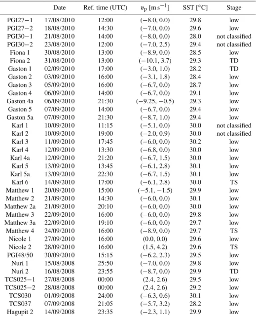
The scatter plots presented in this section consist of data points from 37 cases: 24 from PREDICT, 6 from GRIP and 7 from TCS08. Table 1 shows the date, propagation velocity, reference time, area-averaged Reynolds sea surface temper-ature (SST), and National Hurricane Center (NHC) classifi-cation for each mission conducted into these disturbances. All but two cases observed during PREDICT are included in the scatter plots. The test run from PREDICT has not been entered because the dropsonde pattern did not enclose any area, and the third mission in Fiona is not considered, as its circulation was strongly influenced by hurricane Earl. Each data point represents a single mission into a disturbance of interest.
Table 1. Observational cases that enter the scatter plots in Sect. 5.1. The stage of each disturbance is as recognized by NHC at the time of observation. “Low” stands for either a tropical wave or a weak tropical disturbance, while TD indicates a tropical depression and TS a tropical storm.
Date Ref. time (UTC) vp[m s−1] SST [◦C] Stage
PGI27−1 17/08/2010 12:00 (−8.0, 0.0) 29.8 low PGI27−2 18/08/2010 14:30 (−7.0, 0.0) 29.6 low PGI30−1 21/08/2010 14:00 (−8.0, 0.0) 28.0 not classified PGI30−2 23/08/2010 12:00 (−7.0, 2.5) 29.4 not classified
Fiona 1 30/08/2010 13:00 (−8.9, 0.0) 28.5 low Fiona 2 31/08/2010 13:00 (−10.1, 3.7) 29.3 TD Gaston 1 02/09/2010 17:00 (−3.0, 1.0) 28.2 TD Gaston 2 03/09/2010 16:00 (−3.1, 1.8) 28.4 low Gaston 3 05/09/2010 16:00 (−6.7, 0.0) 28.7 low Gaston 4 06/09/2010 14:00 (−6.7, 0.0) 29.1 low Gaston 4a 06/09/2010 21:30 (−9.25,−0.5) 29.3 low Gaston 5 07/09/2010 14:00 (−6.7, 0.0) 29.4 low Gaston 5a 07/09/2010 21:30 (−8.7, 1.0) 29.4 low
Karl 1 10/09/2010 11:15 (−5.1, 0.0) 30.0 not classified Karl 2 10/09/2010 19:00 (−2.0, 0.9) 30.0 not classified Karl 3 11/09/2010 17:45 (−6.0, 0.0) 30.2 low Karl 4 12/09/2010 13:30 (−6.8, 0.0) 30.0 low Karl 4a 12/09/2010 21:20 (−6.7, 1.5) 30.0 low Karl 5 13/09/2010 13:45 (−6.1, 2.8) 30.1 low Karl 5a 13/09/2010 22:30 (−6.7, 1.5) 30.1 low Karl 6 14/09/2010 17:00 (−6.1, 2.8) 30.0 TS Matthew 1 20/09/2010 15:00 (−5.1,−1.5) 29.9 low Matthew 2 21/09/2010 14:30 (−6.0, 0.0) 30.1 low Matthew 2a 21/09/2010 20:10 (−6.0, 0.0) 30.0 low Matthew 3 22/09/2010 16:00 (−6.0, 0.0) 29.8 low Matthew 3a 22/09/2010 19:10 (−6.0, 0.0) 29.7 low Matthew 4 24/09/2010 16:00 (−8.9, 0.0) 29.7 TS Nicole 1 27/09/2010 16:00 (0.0, 0.0) 29.6 low
Nicole 2 28/09/2010 16:00 (1.5, 4.2) 29.6 TS
PGI48/50 30/09/2010 15:15 (−6.2, 2.3) 29.5 low Nuri 1 15/08/2008 25:50 (−7.0, 0.0) 29.8 low Nuri 2 16/08/2008 23:55 (−8.7, 0.0) 29.9 TD TCS025−1 27/08/2008 00:00 (2.4, 2.6) 29.5 low TCS025−2 28/08/2008 00:00 (2.4, 2.6) 29.2 low TCS030 01/09/2008 24:00 (−6.3, 0.6) 30.1 low TCS037 07/09/2008 21:05 (−5.7, 3.2) 28.2 low Hagupit 2 14/09/2008 23:35 (−2.3, 1.1) 29.9 low
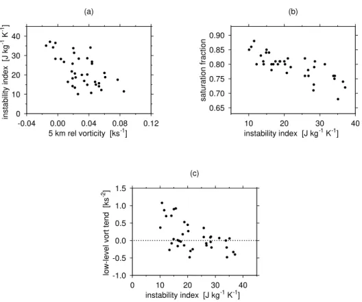
plot suggests that a smaller instability index corresponds to a stronger mid-level vorticity. This result is not surprising be-cause it is in agreement with thermal wind balance: mid-level vorticity is associated with a cooler lower troposphere and/or a warmer upper troposphere, which translates into stabiliza-tion of the atmosphere, that is, a decrease of the instability index.
Figure 1b is a scatter plot of instability index versus satu-ration fraction. It demonstrates negative correlation between these two variables. This tells us that a more stable tropo-sphere tends to be moister. Figure 1c shows a scatter plot between the instability index and the low-level vorticity
ten-dency. The latter is calculated as an average over the lowest kilometer. The negative slope is obvious, which suggests that larger vorticity tendencies are associated with a more stable troposphere. Figure 1b and c suggest that the thermodynam-ics associated with strong mid-level vorticity are conducive to the increase of the near-surface vorticity.
-0.04 0.00 0.04 0.08 0.12 5 km rel vorticity [ks-1] 0
10 20 30 40
instability index [J kg
-1 K
-1]
(a)
10 20 30 40
instability index [J kg-1 K-1] 0.65
0.70 0.75 0.80 0.85 0.90
saturation fraction
(b)
0 10 20 30 40
instability index [J kg-1 K-1] -1.0
-0.5 0.0 0.5 1.0 1.5
low-level vort tend [ks
-2]
(c)
Fig. 1.Scatter plots of(a)mid-level relative vorticity versus instability index,(b)instability index versus saturation fraction, and(c)instability index versus low-level vorticity tendency.
Table 2.Statistics on the scatter plots in Fig. 1.
Variables Correlation coeff. pvalue
Mid-level vorticity vs. instability index 0.32 0.04 Instability index vs. saturation fraction 0.60 0.0002
Instability index vs. low-level vorticity tendency 0.35 0.05
We do not expect strict correlations between the analyzed variables. It is not even clear if the possible correlations that are implied in the scatter plots are linear or not. The con-clusions of our analysis are based solely on the trends that are obvious in the scatter plots presented, positive or neg-ative. Keeping this in mind, one might wonder how strong these correlations are. Assuming linear correlations between all the variables, we conducted statistical analysis on these data. The correlation coefficients and thepvalues are given in Table 2. The significance level is greater than 95 % for all the correlations. The statistics for the analogous scatter plots from the other set of results, where minimal area selection was done, show similar numbers. Therefore, the observed trends in the scatter plots are robust and they strongly sup-port the idea of the mid-level vortex promoting near-surface vorticity intensification via a change in the tropospheric ther-modynamic stratification on the mesoscale. It is true that
cor-relation does not imply causation, but the results of Raymond (2012) strongly imply that the arrow of causality points from the mid-level vortex to the thermodynamics, and not vice versa.
5.2 Karl and Gaston
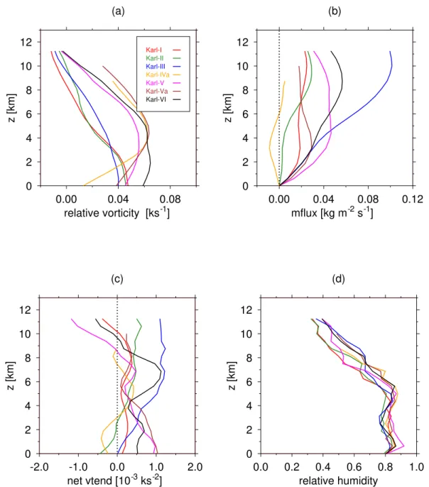
We now analyze the evolution of the vertical profiles of vor-ticity tendency, vertical vorvor-ticity, vertical mass flux, moist en-tropy and saturated moist enen-tropy for Karl and Gaston. The vertical profiles of the analyzed variables represent horizon-tal averages over the respective areas selected for analysis. 5.2.1 Karl
0.00 0.04 0.08
relative vorticity [ks-1]
0 2 4 6 8 10 12
z [km]
Karl-I Karl-II
Karl-III Karl-IVa Karl-V Karl-Va Karl-VI (a)
0.00 0.04 0.08 0.12
mflux [kg m-2 s-1]
0 2 4 6 8 10 12
z [km]
(b)
-2.0 -1.0 0.0 1.0 2.0
net vtend [10-3 ks-2]
0 2 4 6 8 10 12
z [km]
(c)
0.0 0.2 0.4 0.6 0.8 1.0
relative humidity 0
2 4 6 8 10 12
z [km]
(d)
Fig. 2.Horizontally averaged(a)relative vertical vorticity,(b)vertical mass flux,(c)vorticity tendency, and(d)relative humidity for all the Karl missions.
coast. It was a broad low pressure area with active convec-tion. Two observations in this disturbance were conducted before the NHC declared it an area of interest. Thus, the gen-esis phase of Karl, which ultimately developed into a cate-gory 3 hurricane, was well captured.
Because of airspace restrictions, the fourth PREDICT re-search flight did not cover an adequate observational area (the circulation center was not even partly covered) and, therefore, is excluded from the evolution analysis. The re-sults from the other five PREDICT missions and two GRIP missions are summarized in Fig. 2. Karl 1 was conducted on 10 September. The disturbance exhibited weak cyclonic
0 1 2 3 4 5 6 day
10 20 30 40
instab index [J kg
-1 K
-1 ]
(a) Karl
0 1 2 3 4 5 6 7
day 10
20 30 40
instab index [J kg
-1 K
-1 ]
(c) Gaston
0 1 2 3 4 5 6
day 0.00
0.02 0.04 0.06 0.08
vorticity [ks
-1 ]
(b) Karl
0 1 2 3 4 5 6 7
day 0.00
0.02 0.04 0.06 0.08
vorticity [ks
-1 ]
(d) Gaston
Fig. 3.Horizontally averaged(a)relative vertical vorticity,(b)vertical mass flux,(c)vorticity tendency, and(d)relative humidity for all the Gaston missions.
of stratiform clouds, which perhaps resulted as further devel-opment of the convective clouds from earlier that day. The green line in Fig. 2d shows that the relative humidity also decreased in the layer between 1 and 5 km, which is also consistent with the lack of convective clouds. The relative vorticity stayed virtually the same, but the vorticity tendency was negative in the lowest level (green lines in Fig. 2a and c). The vorticity axis maintained a SW tilt.
Bursts of strong convection to the east of the circulation center were observed on 11 September, when the G-V con-ducted its third mission into Karl. The blue lines in Fig. 2 refer to Karl 3. The vertical profile of the relative vorticity shows a slight decrease at low levels and an increase at mid-levels. The vertical mass flux was top-heavy and strong, with a peak near 10 km, resulting in the large positive values of the vorticity tendency at mid-levels. At this point Karl became an area of interest to the NHC. The large mid-level vorticity tendency from Karl 3 resulted in significant mid-level vortic-ity increase, which was observed during the GRIP mission that was conducted on the evening of 12 September (Fig. 2a, orange line). On 13 September, the G-V conducted the fifth mission into the disturbance, which at that time was located over the warm waters of the northwestern Caribbean Sea. At this point Karl had redeveloped the low-level vortex (purple lines in Fig. 2). The relative humidity had increased in the
lowest 3 km. Convection covered a large fractional area of the observational region. Deep convective and stratiform clouds were observed. The vertical mass flux profile was bottom-heavy, reflecting dominance of convective clouds. An asso-ciated large positive vorticity tendency was registered at low levels. The vortex axis was vertical by that time (not shown). A similar situation was observed later that same day (Fig. 2, brown lines). The last PREDICT mission into Karl was con-ducted the following day, when significant low-level vorticity increase was observed (Fig. 2, black line). By the time the G-V returned from this mission, NHC had upgraded Karl to a tropical storm.
Karl kept intensifying; on 16 September, it reached hur-ricane strength, and one day later it became a major hurri-cane. It made a landfall on the Yucatán peninsula, Mexico, and caused significant damage.
0.00 0.04 0.08 relative vorticity [ks-1]
0 2 4 6 8 10 12
z [km]
Gaston-I Gaston-II Gaston-III Gaston-IV Gaston-IVa Gaston-V Gaston-Va
(a)
0.00 0.04 0.08 0.12
mflux [kg m-2 s-1]
0 2 4 6 8 10 12
z [km]
(b)
-2.0 -1.0 0.0 1.0 2.0
net vtend [10-4 ks-2]
0 2 4 6 8 10 12
z [km]
(c)
0.0 0.2 0.4 0.6 0.8 1.0
relative humidity 0
2 4 6 8 10 12
z [km]
(d)
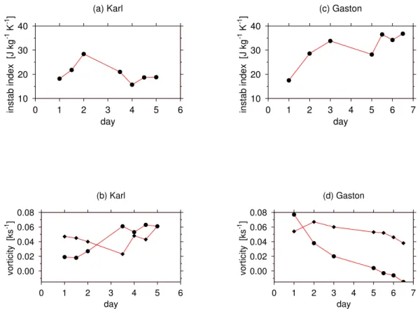
Fig. 4.Karl (left column) and Gaston (right column). The upper panels show the time series of the instability index. The solid circles in the lower panels are for the mid-level relative vorticity and the diamonds are for the low-level relative vorticity.
1 of observation was low, but it increased between the first two missions into Karl. During that time, the mid-level vor-tex was not well developed and it was weaker than the low-level vortex. By the third mission the mid-low-level vorticity had slightly increased, but most importantly, the instability in-dex had further increased. A corresponding strong, top-heavy mass flux profile was observed (Fig. 2b, blue line), which is in agreement with the theoretical results of Raymond and Sessions (2007). As a response to this mass flux profile of Karl 3, the following day significant mid-level vortex inten-sification was observed, as was a corresponding decrease of the instability index. From here, the low-level vortex started intensifying as well, and in less than 48 h Karl became a trop-ical storm.
5.2.2 Gaston
-44 -42 -40 -38 long
12 14 16
lat
5 m/s
(a) Gaston 1: 5 km
-46 -44 -42 -40 -38
long 12
14 16
lat
0.0 0.2 0.4 0.6 0.8 1.0
5 m/s
(b) Gaston 2: 5 km
-44 -42 -40 -38
long 12
14 16
lat
5 m/s
(c) Gaston 1: 7 km
-46 -44 -42 -40 -38
long 12
14 16
lat
0.0 0.2 0.4 0.6 0.8 1.0
5 m/s
(d) Gaston 2: 7 km
Fig. 5.Relative humidity during Gaston 1 (left panels) and Gaston 2 (right panels) at 5 km and at 7 km. The vectors represent the relative wind at the respective levels. The red boxes enclose the area selected for analysis.
Gaston 2 was conducted the following day. The green lines in Fig. 3 show the area-averaged vertical structure of Gas-ton 2. The most obvious feature is that the relative vorticity changed drastically from the previous day, even though a vor-tex was still evident (Fig. 5b). The low-level vorticity, how-ever, was greater, in spite of the negative vorticity tendency from the previous day. This disagreement is most likely due to the fact that the vorticity tendency equation only provides a snapshot at a particular time. The vertical mass flux pro-file at this time exhibited a maximum near 4 km, but the convective regions covered a smaller fractional area of the disturbance than the downdrafts, so that the magnitude of area-averaged vertical mass flux had not changed from the previous day. The area-averaged relative humidity remained almost the same. By the next day (Gaston 3), the relative vor-ticity decreased at all levels and also the relative humidity de-creased notably (Fig. 3a, d; blue lines). The rest of the mis-sions conducted in this disturbance revealed a further trend of decrease in relative vorticity and relative humidity.
Figure 4 summarizes the evolution of the thermodynam-ics and dynamthermodynam-ics for Gaston during the period it was ob-served. At time 1, Gaston featured a low instability index and a strong mid-level vortex. According to our theory, this is favorable for low-level vorticity increase, which did in-deed happen by time 2. However, in the period between 1 and 2, a significant decrease in mid-level vorticity and a
cor-responding increase in the instability index occurred. After time 2, the relative vorticity at both low and middle levels decreased continuously, while the instability index was in-creased. Smith and Montgomery (2012) also found that, as Gaston was decaying, Convective Available Potential Energy (CAPE) was increasing.
5.2.3 What caused Gaston to decay?
-44 -42 -40 -38 lon
Fig. 6.Vertical mass flux and relative wind at 3 km and at 6 km for Gaston 1 (left panels) and Karl 3 (right panels). The units are kg m−2s−1. The red boxes enclose the area selected for analysis, and the black boxes enclose the area of convective activity.
of Gaston’s evolution. We do not question the existence of dry air intrusion after Gaston 2. As the above cited papers showed, and as is reflected in our Fig. 5b, the drying of the disturbance started after the second mission into it.
We hypothesize that the severe decrease of the mid-level vortex observed in the period between Gaston 1 and Gaston 2 was a deciding factor for Gaston’s failure to re-intensify (see Fig. 3a). Therefore, in this section we explore possible fac-tors that caused this dissipation. We also compare Gaston 1 and Karl 3, as we find that events observed in these two mis-sions were critical to the subsequent success or failure of the respective systems, and the contrast between the two is in-structive.
The decrease in the mid-level vorticity from Gaston 1 to Gaston 2 we find to be due to the form of the vertical mass flux profile observed during Gaston 1. The left panels in Fig. 6 show the vertical mass flux at 3 km and at 6 km ele-vation for Gaston 1. Positive vertical mass flux existed near the circulation center in Gaston. However, it was weak in the upper troposphere and it covered a small area. The right pan-els in Fig. 6 show analogous plots for Karl 3. Convection in Karl 3 was stronger at higher levels and it covered a much larger area compared to that of Gaston 1. The black boxes in this figure enclose most of the convective activity.
0.00 0.05 0.10 0.15 mflux [kg m-2 s-1] 0
2 4 6 8 10 12
z [km]
(a) Gaston 1
0.00 0.05 0.10 0.15 mflux [kg m-2 s-1] 0
2 4 6 8 10 12
z [km]
(b) Karl 3
Fig. 7.Vertical mass flux profiles averaged over the black boxes in Fig. 6 for Gaston 1 (left) and Karl 3 (right).
-44 -42 -40 -38
lon
Fig. 8.Reynolds SST (units are◦C) for Gaston 1 (left) and Karl 3 (right). The vectors represent the relative wind, averaged over the lowest kilometer. The purple dots indicate dropsonde positions, and the yellow diamond marks the circulation center at 5 km.
profile during Gaston 1. Therefore, what is the reason for such convection during Gaston 1?
Why was the Gaston 1 mass flux profile so different from that of Karl 3? There are three possibilities for this. First, dry air might have been drawn into the core of Gaston; second, the surface fluxes were likely weaker; and third, buoyancy adjustment from the surroundings may have stabilized the convective column in Gaston. The first possibility is unlikely, as discussed above, due to the robust pouch in Gaston 1.
The underlying ocean provides surface heat fluxes into the disturbance. A warmer ocean provides more energy in the atmosphere. Figure 8a shows the Reynolds SST for Gas-ton 1. The overlying vector field is the system-relative wind averaged between 0 and 1 km. The SST below the circula-tion center is∼28.5◦C and it decreases northward. Though these SSTs are above the threshold for tropical storm devel-opment, they are 2◦C cooler then the corresponding SSTs for Karl 3 (Fig. 8b). The stated threshold does not ensure de-velopment and 2◦C difference in SST can make a large dif-ference in surface fluxes. Furthermore, in recent years stud-ies have found that the underlying upper ocean heat
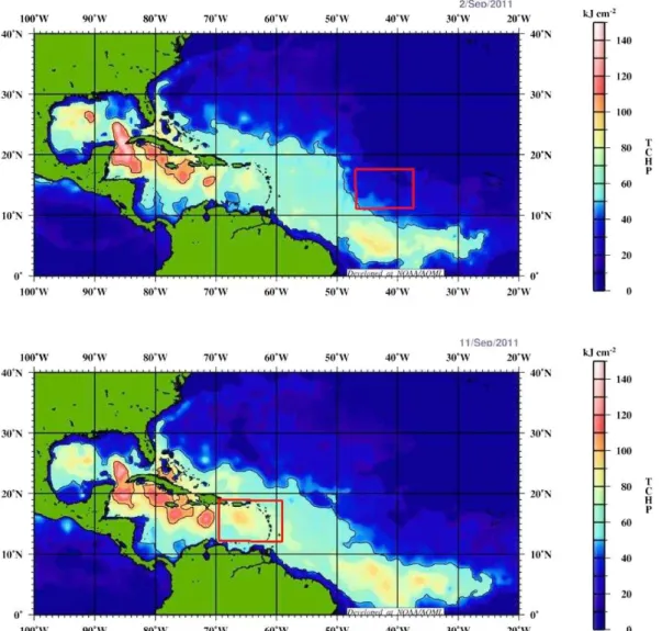
con-tent, rather then the SST, is a better representative of the ocean’s input into the disturbance. The higher the heat con-tent, the higher the transport from the ocean to the atmo-sphere (Wada and Usui, 2007). Figure 9 is taken from Na-tional Oceanic and Atmospheric Administration’s (NOAA) website and it shows the Tropical Cyclone Heat Potential (TCHP), a variable representative of the ocean heat content. Roughly estimated from the figure, the average TCHP for Gaston 1 is less then 40 kJ cm−2. For Karl 3 the average is around 80 kJ cm−2, with largest values of 100 kJ cm−2, ap-proximately collocated with the circulation center of the dis-turbance. This large difference in TCHP is potentially an im-portant factor for the observed differences in the mass flux profiles of Gaston 1 and Karl 3.
Fig. 9.TCHP for Gaston 1 (top panel) and Karl 3 (bottom panel). The red boxes mark approximately the respective observational areas. The graphics are taken from http://www.aoml.noaa.gov/phod/cyclone/data.
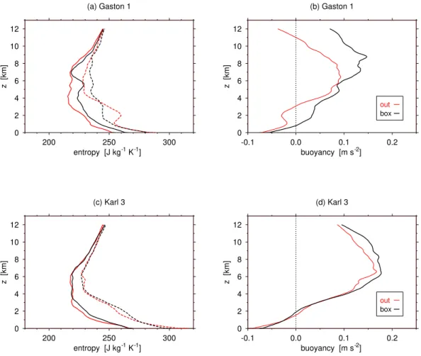
the dropsondes outside these regions, but still within the se-lected area for analysis. The results are shown in Fig. 10. The saturated moist entropy for Gaston 1 indicates a tem-perature inversion. The inversion is especially evident out-side the black box, even though it is present within the black box as well (Fig. 10a, red dashed red line and black dashed line, respectively). Within the convectively active region the buoyancy profile does not show evidence of an inversion (Fig. 10b), most likely because convection locally destroys the inversion. Outside the black box in Gaston 1, both sat-urated moist entropy and buoyancy indicate a strong trade wind inversion and overall a much smaller magnitude of buoyancy. In contrast, the corresponding entropy and buoy-ancy vertical profiles of Karl 3 (Fig. 10 c and d) show no evidence of an inversion inside or outside of the convectively active region, which is consistent with the high values of the underlying SSTs. There is a notable difference between the
buoyancy profiles of Gaston 1 and Karl 3. For Gaston 1 there is a big difference in buoyancy within and outside the con-vectively active region, whereas for Karl 3, this difference is much smaller. Thus, the larger environment (outside the box) for Karl 3 is conducive to convection, whereas for Gaston 1 it is very unfavorable. We hypothesize that in Gaston 1 convec-tion is modifying buoyancy locally, and thus the inversion is reduced in the region of convective activity, while at the same time the trade wind dynamics are reinforcing the temperature inversion, which tends to suppress convection.
200 250 300 entropy [J kg-1 K-1] 0
2 4 6 8 10 12
z [km]
(a) Gaston 1
-0.1 0.0 0.1 0.2
buoyancy [m s-2] 0
2 4 6 8 10 12
z [km]
out box (b) Gaston 1
200 250 300
entropy [J kg-1 K-1] 0
2 4 6 8 10 12
z [km]
(c) Karl 3
-0.1 0.0 0.1 0.2
buoyancy [m s-2] 0
2 4 6 8 10 12
z [km]
out box (d) Karl 3
Fig. 10. Vertical profiles of(a)moist entropy (solid lines) and saturated moist entropy (dashed lines) for Gaston 1,(b)buoyancy for Gaston 1, (c)moist entropy (solid lines) and saturated moist entropy (dashed lines) for Karl 3, and(d)buoyancy for Karl 3. The black lines represent averages over the dropsondes inside the respective black boxes in Fig. 8, and the red lines represent averages over the dropsondes enclosed with the respective red box, but outside of the black boxes in Fig. 8.
to Gaston 2. This led to the collapse of the pouch at mid-levels and the subsequent intrusion of dry air into Gaston’s core, resulting in its failure to develop. Low relative humid-ity above 6 km may have been an additional factor, but this effect was likely weak due to the low saturation mixing ratio and hence low saturation deficit at high elevations. Dry air surrounded Gaston at middle levels, but initially appeared to be unable to penetrate to the core due to the protective pouch produced by the mid-level vortex, thus limiting its direct ef-fect on convection during Gaston 1.
6 Conclusions
This paper uses observations from three field programs to ex-plore tropical storm formation. Possible correlations between dynamics and thermodynamics were explored in Sect. 5.1 and detailed analyses of two disturbances observed during PREDICT were presented in section 5.2. The vertical pro-files of the various variables presented represent areal aver-ages. Because of airspace restrictions some of the
observa-tional domains were not centered over the target disturbance. Thus, the vertical profiles most likely differ from what they would be if averaged over the exact area that the respective disturbances cover. Given the small timescales and horizontal scales of convection versus the larger timescales and horizon-tal scales of mesoscale vorticity, the mean vertical vorticity profile is probably much less sensitive to the domain selec-tion than the mass flux profile. Therefore, it is more robust in representing the big picture of the disturbance behavior, unless the circulation center is entirely outside of the ob-servational domain. Missions where the latter was the case do not enter the analyses in Sect. 5.2. Davis and Ahijevych (2012) have used other data sources in addition to the drop-sonde data and have used a different treatment in calculating the vertical circulation profiles of their analyses of Gaston, Karl and Matthew. The results they obtained do not differ qualitatively from the results presented in this paper which reinforces our analysis.
mid-level vortex preceded low-level vortex intensification in the developing case, and divergence of mid-level vorticity preceded weakening of the low-level vortex in the decaying case. The important question that we attempt to answer in this paper is how the mid-level vortex communicates with the dynamics at low levels. The evolution of the dynamics and thermodynamics of Karl and Gaston, the trends in the scat-ter plots, and the previous theoretical work by Raymond and Sessions (2007), support the following theory on the mecha-nisms by which the mid-level vortex promotes low-level spin up: by virtue of thermal wind balance, the mesoscale mid-level vortex maintains a more stable atmosphere. We saw from observations that stronger mid-level vorticity was in-deed associated with a lower instability index (Fig. 1a). The more stable atmosphere is conducive to moist convection that produces a bottom-heavy mass flux profile, meaning that it exhibits the largest positive vertical gradient in a shallow layer adjacent to the sea surface. Mass continuity then dic-tates horizontal mass convergence at low levels, where most of the water vapor is contained. Mass convergence near the surface means water vapor convergence and low-level vor-ticity convergence. Hence the negative correlations between the instability index and the saturation fraction (Fig. 1b) and between the instability index and the low-level vorticity ten-dency (Fig. 1c). If the mid-level vorticity exists long enough to keep this chain of events going, the low-level wind speed will eventually reach the tropical storm threshold.
The theory presented here is in agreement with the marsu-pial paradigm that the low-level vortex intensifies as a result of the aggregation of vorticity produced by deep convection. Our theory focuses on the vertical mass flux that most effi-ciently leads to aggregation of vorticity. From observations, we found that it is a mass flux with the strongest positive ver-tical gradient in a shallow layer near the surface. Our theory says that the mid-level vortex is necessary to maintain ther-modynamic stratification on the mesoscale that is conducive to such convection. We believe that the protective pouch, de-fined by the marsupial paradigm, also plays an important role in supporting convection in that it blocks the ingestion of dry environmental air into the convective region. Furthermore, the mid-level vortex is instrumental in creating the mid-level pouch, and, as Gaston illustrates, its absence facilitates the ingestion of environmental air.
Karl was a disturbance that closely followed our theory. It was observed in the 4-day period before it become a tropi-cal storm. It started with a low-level cyclonic vortex and a weaker mid-level vortex, but it did not start intensifying un-til it developed a strong mid-level vortex. The development of the mid-level vortex followed as a result of the strong, top-heavy vertical mass flux profile that was observed dur-ing Karl 3. This profile is consistent with the high instability index that existed at that time. Karl 5 exhibited strong mid-level vorticity and a low instability index which resulted in low-level vortex spin up between Karl 5 and Karl 6.
Gaston was first observed only a couple of hours after it decayed from a tropical storm to a tropical depression. Dur-ing this period, Gaston still had a strong mid-level vortex, which had weakened significantly by the second mission into this disturbance. We believe that this was the crucial element in Gaston’s decay. We further hypothesize that convection was suppressed by a strong trade wind inversion. Convection at the time of the observation was concentrated in a small area near the 5 km circulation center. It produced a bottom-heavy vertical profile of the convective mass flux, which de-creased with altitude in the middle troposphere. Though the bottom-heavy mass flux profile produced a transient inten-sification of the low-level vortex, the negative vertical gra-dient of the mass flux above 3 km was responsible for the negative vorticity tendency in the middle levels and therefore the decrease in mid-level vorticity by the following day. The divergence of the mid-level vorticity exposed Gaston to the ingestion of dry environmental air, which sealed its fate.
Acknowledgements. We thank the dedicated staff of the
NSF/NCAR G-V operation for their excellent work. Data provided by NCAR/EOL under sponsorship of the National Science Foundation. This work was supported by National Science Foundation grants 0851663 and 1021049, and the Office of Naval Research grant N000140810241.
Edited by: T. J. Dunkerton
References
Bister, M. and Emanuel, K. A.: The genesis of hurricane Guillermo: TEXMEX analyses and a modeling study, Mon. Weather Rev., 125, 2662–2682, 1997.
Braun, S. A., Kakar, R., Zipser, E., Heymsfield, G., Albers, C., Brown, S., Durden, S. L., Guimond, S., Halverson, J., Heyms-field, A., Ismail, S., Lambrigsten, B., Miller, T., Tanelli, S., Thomas, J., and Zawislak, J.: NASA’s Genesis and Rapid Intensi-fication Processes (GRIP) field experiment, B. Am. Meteor. Soc., 94, 345–363, 2012.
Davis, C. A., and Ahijevych, D. A.: Mesoscale structural evolution of three tropical weather systems observed during PREDICT, J. Atmos. Sci., 69, 1284–1305, 2012.
Dunkerton, T. J., Montgomery, M. T., and Wang, Z.: Tropical cy-clogenesis in a tropical wave critical layer: easterly waves, At-mos. Chem. Phys., 9, 5587–5646, doi:10.5194/acp-9-5587-2009, 2009.
Gray, W. M.: Global view of the origin of tropical disturbances and storms, Mon. Weather Rev., 96, 3380–3403, 1968.
Haynes, P., and McIntyre, M.: On the evolution of vorticity and po-tential vorticity in the presence of diabatic heating and fractional or other forces. J. Atmos. Sci., 44, 828–841, 1987.
Harr, P. A., and Elsberry, R. L.: Transformation of a large monsoon depression to a tropical storm during TCM-93, Mon. Weather Rev., 124, 2625–2643, 1996.
ef-ficient two-step approach, Atmos. Meas. Tech., 4, 2717–2733, doi:10.5194/amt-4-2717-2011, 2011.
McBride, J. L., and Zehr, R.: Observational analysis of tropical cy-clone formation. Part II: Comparison of non-developing versus developing systems, J. Atmos. Sci., 38, 1132–1151, 1981. Montgomery, M. T., Davis, C., Dunkerton, T., Wang, Z., Velden,
C., Torn, R., Majumdar, S. J., Zhang, F., Smith, R. K., Bosart, L., Bell, M. M., Haase, J. S., Heymsfield, A., Jensen, J., Campos, T., and Boothe, M. A.: The Pre-Depression Investigation of Cloud-systems in the Tropics (PREDICT) experiment, B. Am. Meteor. Soc., 93, 153–172, 2012.
Montgomery, M. T. and Smith, R. K.: The genesis of Typhoon Nuri as observed during the Tropical Cyclone Structure 2008 (TCS08) field experiment – Part 2: Observations of the convective environ-ment, Atmos. Chem. Phys., 12, 4001–4009, doi:10.5194/acp-12-4001-2012, 2012.
Nolan, D. S.: What is the trigger for tropical cyclogenesys?, Aust. Met. Mag., 56, 241–266, 2007.
Raymond, D. J.: Balanced thermal structure of an in-tensifying tropical cyclone, Tellus-A, 64, 19181, doi:10.3402/tellusa.v64i0.19181, 2012.
Raymond, D. J. and López Carrillo, C.: The vorticity budget of de-veloping typhoon Nuri (2008), Atmos. Chem. Phys., 11, 147– 163, doi:10.5194/acp-11-147-2011, 2011.
Raymond, D. J. and Sessions, S. L.: Evolution of convection dur-ing tropical cyclogenesis, Geophys. Res. Lett., 34, L06811, doi:10.1029/2006GL028607, 2007.
Raymond, D. J., Sessions, S. L., and López Carrillo, C.: Thermody-namics of tropical cyclogenesis in the Northwest Pacific, J. Geo-phys. Res., 116, D18101, doi:10.1029/2011JD015624, 2011. Reasor, P. D., Montgomery, M. T., and Bosart, L. F.:Mesoscale
ob-servations of the genesis of Hurricane Dolly (1996), J. Atmos. Sci., 62, 3151–3171, 2005.
Rutherford, B. and Montgomery, M. T.: A Lagrangian analysis of a developing and non-developing disturbance observed during the PREDICT experiment, Atmos. Chem. Phys., 12, 11355–11381, doi:10.5194/acp-12-11355-2012, 2012.
Smith, R. K. and Montgomery, M. T.: Observations of the convec-tive environment in developing and non-developing tropical dis-turbances, Q. J. Roy. Meteorol. Soc., 138, 1721–1739, 2012. Wada, A. and Usui, N.: Importance of tropical cyclone heat
poten-tial for tropical cyclone intensity and intensification in the west-ern north pacific, J. Oceanogr., 63, 427–447, 2007.
Wang, Z.: Thermodynamic Aspects of Tropical Cyclone Formation, J. Atmos. Sci., 69, 2433–2451, 2012.
Appendix A
Buoyancy calculation
We calculate the buoyancy as follows:
b= −g(Tv−Tvp)/Tv. (A1)
Tvis the environmental virtual temperature,
Tv=T (1+0.00061r), (A2)
andTvpis the parcel virtual temperature,
Tvp=Tp(1+0.00061rp). (A3)
Tpis the parcel temperature at each level and it is calculated
as the environmental temperature plus a temperature pertur-bation,δT, of the parcel at each level. The latter is estimated by using the approximate formulas (7) and (8) from RSL11. These are
δT =δs∗/(∂s∗/∂T )p≈δs∗/(3.7+0.00064r∗), (A4) where we calculateδs∗as
δs∗=s∗−s0. (A5)
Heres0is the specific moist entropy averaged over the lowest
kilometer ands∗is the saturated moist entropy of the envi-ronment. The variablerp=rp(z)in Eq. (A3) is the mixing
ratio of the parcel, which we calculate from the pressure and Tp, on the assumption that the parcel is saturated. We use the
formula rp=0.622
es(Tp)
p−es(Tp)
, (A6)
whereesis the saturation vapor pressure calculated from the