Constrained Probabilistic Lost Sales Inventory System with Normal Distribution and Varying Order Cost

(1)

Journal of Mathematics and Statistics 2 (1): 363-366, 2006 ISSN 1549-3644

Corresponding Author: Hala, A. Fergany, Department of Mathematical Statistics, Faculty of Science, Tanta University, Tanta, Egypt

363

Constrained Probabilistic Lost Sales Inventory System with

Normal Distribution and Varying Order Cost

1

Hala, A. Fergany and

2

Mona, F. EL-Wakeel

1

Department of Mathematical Statistics, Faculty of Science, Tanta University, Tanta, Egypt

2

Higher Institute for Computers, Information and Management Technology, Tanta, Egypt

Abstract: This study derives the probabilistic lost sales inventory system when the order cost is a function of the order quantity. Our objective is to minimize the expected annual total cost under a restriction on the expected annual holding cost when the lead-time demand follows the normal distribution by using the Lagrangian method. Then a published special case is deduced and an illustrative numerical example is added.

Key words: Probabilistic model lost sales inventory system, varying order cost, lead-time demand INTRODUCTION

Continuous review<Q,r>inventory models with constant units of cost and stationary distributions of inventory level have been studied by Feldman[1], Richards[2] and Sahin[3].The inventory models under continuous review with stationary distribution of inventory level have been derived using renewal theory given by Arrow[4]. Also, Fabrycky[5] studied the probabilistic single- item, single source(SISS) inventory system with zero lead-time, using the classical optimization. Fergany[6,7] discussed constrained probabilistic inventory model with varying order and shortage costs using Lagrangian method and constrained probabilistic single- item inventory problem with varying order cost using geometric programming. Abou-El-Ata[8] introduced a probabilistic multi-item inventory model with varying order cost, zero lead time under two restriction. Hadley[9] and Taha[10] discussed unconstrained probabilistic continuous review inventory models with constant units of cost. Ben-Daya[11] examined unconstrained inventory model with constant units of cost, demand follows a normal distribution and the lead-time is one of the decision variables. Recently, Fergany[12] studied constrained probabilistic inventory model with continuous distributions and varying holding cost.

This study considering a continuous review model with lost sales case, varying order cost, a restriction on the expected annual holding cost and the lead-time demand follows normal distribution. The policy variables of this model are the order quantity and the reorder level, which minimize the relevant annual total cost. Finally, a special case is deduced, which has been previously published and a numerical illustrative example is added.

Notations and assumptions: The following notations are adopted for developing our model:

D = The average rate of annual demand, Q = A decision variable representing the order quantity per cycle,

r = A decision variable representing the reorder point, N = The inventory cycle,

Nˆ =The average length of time per cycle when the

system is out of stock,

n = The average number of cycles per year,

L = The lead-time between the placement of an order and its receipt,

x = The continuous random variable represents the demand during L (lead-time demand),

f(x) = The probability density function of the lead-time demand and F(x) its distribution function,

r-x = The random variable represents the net inventory when the procurement quantity arrives

if the lead-time demand x≤r,

E(r-x) = ss= Safety stock= The expected net inventory = −

r

dx x f x r 0

) ( )

( =

∞

− + −

r

dx x f r x x E

r ( ) ( ) ( ) ,

H = The average on hand inventory =

2 . .onhand Minonhand

Max +

=

∞

− + − + = + +

r

dx x f r x x E r Q ss Q ss

) ( ) ( ) ( 2

2 ,

R(r) = The reliability function = 1-F(x)=

∞

r dx x f( ) ,

) (r

S =The expected value of lost sales per cycle =

∞

− r

dx x f r x ) ( )

( ,

o

(2)

J. Math. & Stat. 2 (1): 363-366, 2006

364

β

Q c Q

Co( )= o =The varying order cost per cycle,

1

0<

β

< , where

β

is a constant real number selected to provide the benefit of estimated expected cost function,

h

c = The holding cost per year, l

c = The lost sales cost per cycle,

K = The limitation on the expected annual holding cost. The system is a continuous review, which means that the demands are recorded as they occur and the stock level is known at all times. An order quantity of size Q per cycle is placed every time the stock level reaches a certain reorder point r(Q and are two decision variables). For the lost sales case, the average number of cycles per year is given by: n D _ˆ

Q DN

=

+ . In

the real world ˆN is usually a very small fraction of the total length of the cycle, then it is inconvenient to include ˆNin the analysis, the following assumptions are usually made in the simple treatments for developing the mathematical model:

* The cycle is defined as the time between two successive arrival of orders and assume that the system repeats itself in the sense that the inventory position varies between r and r+Qduring each cycle as it illustrated in Fig. 1.

* The average number of cycles per year can be written as n D

Q

= and then the inventory cycle isN Q

D

= .

* The unit cost c_P of the item is a constant independent ofQ.

* There is never more than a single order outstanding.

N Time

Q r

In

v

e

n

to

ry

l

e

v

e

l

Fig. 1:The behavior of the continuous review system with

lost sales case

Relevant expected annual total cost: Using the expression of the expected value of a random variable, it is possible to develop the expected annual total cost as follows:

E( Total Cost ) = E( Order Cost )+ E( Holding Cost )+ E(Lost Sales Cost ).

I.e., (E TC)=E OC( )+E HC( )+E LC( ) (1)

Where ₍ ₎ _{( ).} 1

o o o

D E OC C Q n c Q c DQ

Q

β β −

= = = (2)

( ) ( ) ( ) ( )

2

h h

r Q

E HC c H c r E x x r f x dx

∞

= = + − + − (3)

and ( ) . . ( ) l ( ) ( )

l

r

c D

E LC c n S r x r f x dx Q

∞

= = − (4)

Therefore

[

]

1

( , ) ( )

2

( ) ( )

o h

l h

r

Q

E TC Q r c DQ c r E x

c D

c x r f x dx Q

β−

∞

= + + −

+ + −

(5)

our objective is to minimize the expected annual total cost E TC Q r

[

( , )

]

under the following constraint:

( ) ( ) ( )

2 h

r

Q

c r E x x r f x dx K

∞

+ − + − ≤ (6)

To solve this primal function, which is a convex programming problem, let us write it in the following form:

[

]

1

( , )

( ) ( )

2

o h

l h

E TC Q r c DQ c

c D Q

r E x c S r

Q

β−

= +

+ − + + (7)

subject to: ( ) ( )

2 h

Q

c + −r E x +S r ≤K (8)

To find the optimal values *

Q and *

r which

minimize equation (7) under the constraint (8), we will use the Lagrange multiplier technique as follows:

1

( , , ) ( )

2

( ) ( ) ( )

2

o h

l

h h

Q

L Q r c DQ c r E x

c D Q

c S r c r E x S r K Q

β λ

λ −

= + + −

+ + + + − + −

(9)

Where λ is the Lagrangian multiplier.

The optimal values *

Q and *

r can be found by

setting each of the corresponding first partial derivatives of equation (9) equal to zero, then we obtain:

2

2 ( ) 0

AQ −B Qβ − G S r = (10) and

* *

( ) A Q

R r

G A Q

=

+ (11)

whereA=(1+λ)c_h , B=2 (1−β)c D_o and G=c D_l

(3)

J. Math. & Stat. 2 (1): 363-366, 2006

365 * Step 1: Assume that S =0 and r=E x( ), then from equation (10) we have:

1 2 1

B Q

A

β

−

= (12)

* Step2: Substituting from equation (12) into equation (11) we get:

1 1

2 2

1 1 1

2 2

( ) A B

R r

G A B

β

β β

β

β β

−

− −

−

− −

= +

(13)

* Step 3: Substituting by r1 from equation (13) into

equation (10) to find Q₂ as:

2

2 2 2 ( )1 0

A Q −B Qβ − G S r = (14)

The procedure is to varyλ in equations (13) and (14) until the smallest value of .λ >0 is found such that the constraint holds for the different values of ß.

* Step 4: Repeating the steps 2 and 3 until obtaining

successive values of Q and r, such that they are sufficiently close, which are the optimal values.

The model with normally lead-time demand:

Assume that the lead-time demand follows the Normal distribution. So we can minimize the expected annual total cost mathematically as follows:

( )

2 1 2

2

1

( ) ; 0,

2

with ( ) , var( )

( ) ,

consider

x

f x e x

E x x

r R r Z where Z

µ σ

σ π

µ σ

− −

= ≥

= =

−

= Φ =

and S r( )=(µ−r)Φ

( )

Z +σ φ

( )

Z (15)

where

( )

2 1 2

1 2

Z

Z e

φ

π

−

= and

( )

z

Z φ x dx ∞

Φ =

Substituting form (15) into (10) and (11), we get:

( )

2

2 ( ) 0

A Q −B Qβ− G µ−r Φ Z +σ φ Z = (16) and

_{( )}

* * A Q Z

G A Q

Φ =

+ (17)

For solving the pairs of equations (16) and (17), we have to use the previous iterative method.

Special Case:

Letβ =0 and K→ ∞ C Q_o( )=c_o and λ=0. Thus equations (16) and (17) become:

* 2 [ o l ( )]

h

D c c S r Q

c

+

= (18)

and

* *

*

h

l h

c Q r

c D c Q

µ σ

−

Φ =

+ (19)

This is unconstrained lost sales inventory model with lead-time demand follows the normal distribution and constant order cost as given by Hadley[9].

An illustrative example:

A large military installation stocks a special purpose vacuum tube for use in radar sets. The average annual demand for this tube is 1600 units. Each tube costs $50. The tube must be made to order and hence each time an order is placed it is necessary to go through a process of accepting bids and negotiating a contract. It is estimated that the cost of placing an order is $4000, the installation uses an inventory carrying charge of 0.20. It has been found that if a demand occurs when the system is out of stock; it is possible to obtain such a tube from a small stock carried at one of the manufacturers. However, the cost of sending a plane there to obtain it and the other concomitant expenses amount to $2000 over the cost of the unit. An empirical investigation has shown that the distribution of lead-time demand is essentially normally distributed with mean 750 units and standard deviation 50 units. The inventory is controlled using a <Q, r> system under the constraint that the average holding cost is either less than or equal $8500 per year. It is desired to compute the optimal order quantity and the reorder point.

Solution: The description of the operation of the system presented above indicates that we here need the model for the lost sales case. The iterative procedure that discussed above will be used to solve the equations

(19) and (20) and then obtain the optimal values *

Q and

*

r for varying values of λ and ß as in Table 1.

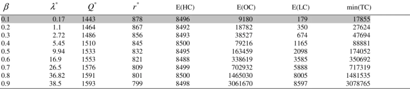
Table 1: The optimal solutions and the min E(TC) when lead-time demand follows normal distribution

β *

λ *

Q r* E(HC) E(OC) E(LC) min(TC)

0.1 0.17 1443 878 8496 9180 179 17855

0.2 1.1 1464 867 8492 18782 350 27624

0.3 2.72 1486 856 8493 38527 674 47694

0.4 5.45 1510 845 8500 79216 1165 88881

0.5 9.94 1533 832 8495 163459 2098 174052

0.6 16.9 1553 821 8488 338619 3585 350692

0.7 26.5 1576 809 8499 702932 5888 717319

(4)

J. Math. & Stat. 2 (1): 363-366, 2006

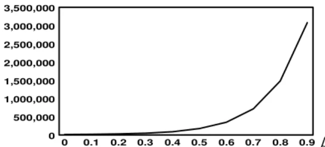
366 From Table 1, we can draw each of E (OC) and

mine (TC) against ß as shown in Fig. 2 and 3:

E(OC)

0 0.1 0.2 0.3 0.4 0.5 0.6 0.7 0.8 0.9 0

500,000 1,000,000 1,500,000 2,000,000 2,500,000 3,000,000 3,500,000

β

Fig. 2:The corresponding values of E (OC) with varying values of ß

E(TC

)

0 0.1 0.2 0.3 0.4 0.5 0.6 0.7 0.8 0.9 0

500,000 1,000,000 1,500,000 2,000,000 2,500,000 3,000,000 3,500,000

β

Fig. 3:The values of E (TC) for normal lead-time demand at each

value of ß

CONCLUSION

For the probabilistic lost sales case with varying order cost and the lead-time demand follows normal distribution under a constraint on the expected annual holding cost, we can not find the exact solution directly but we can evaluate the solution of and or different value of and ß by using the iterative method and then obtain the minimum expected total cost. So we can deduce that the least minimum expected total cost will be held at the least value of ß.

REFERENCES

1. Feldman, R.M., 1978. A Continuous Review (s,S) Inventory System In A Random Environment. J. Appl. Prob., 15: 654-659.

2. Richards, F.R., 1975. Comments On The

Distribution Of Inventory Position In A

Continuous Review (s, S) Inventory System. Operat. Res., 23: 366-371.

3. Sahin, I., 1979. On The Stationary Analysis Of Continuous Review (s, S) Inventory Systems And Constant Lead-Times. Operat., Res., 27: 717-729. 4. Arrow, K.J., S. Karlin and H. Scarf (Eds.), 1958.

Studies In Mathematical Theory Of Inventory And Production. Stanford University Press, Stanford, CA.

5. Fabrycky, W.J. and J. Banks, 1967. Procurement and Inventory System: Theory and Analysis. Reinhold Publishing Corporation, USA.

6. Fergany, H.A., 1999. Inventory Models With Demand-Dependent Unit Cost. Ph.D. Thesis. Faculty of Science, Tanta University, Egypt. 7. Fergany, H.A. and M.F. El-Wakeel, 2004.

Probabilistic Single-Item Inventory Problem With Varying Order Cost Under Two Linear Constraints. J. Egypt. Math. Soc., 12: 71-81.

8. Abou -Ata, M.O., H.A. Fergany and M.F. El-Wakeel, 2003. Probabilistic Multi- Item Inventory Model With Varying Order Cost Under Two Restrictions: A Geometric Programming Approach. Intl. J. Product. Econ., 83: 223-231.

9. Hadley, G. and T.M. Whitin, 1963. Analysis of Inventory Systems. N.J. Prentice Hall, Englewood Cliffs.

10. Taha, H., 1997. Operations Research. N.J. Prentice Hall, Englewood Cliffs, 6th Edn.

11. Ben-Daya, M. and A. Raoyf, 1994. Inventory Models Involving Lead-Time As A Decision Variable. J. Oper. Res. Soc., 45: 579-582.

12. Fergany, H.A and M.E. El-Saadani, 2005. Constrained Probabilistic Inventory Model With Continuous Distributions And Varying Holding Cost. Intl. J. Appl. Math., 17: 53-67