! "# $ % # &
'() * +' ,,+)- . ('/0)0)+ . )/ 1 ()2 3'
+)/, 3,2) ' 4 ($/') ' ($3. )/ .). ,/-) $ )./)
1Department of Industrial Engineering University of Payame
Noor19395 4697, Tehran, I.R. of Iran
2School of Information Technology, Faculty of Information Science and Technology,
Universiti Kebangsaan Malaysia, 43600 Bangi, Selangor, Malaysia *Corresponding author: [email protected]
Abstract
This paper investigates the effect of inflation and time value of money on an economic production quantity (EPQ) model in the single product system while the shortage of inventory is not allowed and production of defective parts during the production process and also setup time for reworking have been considered that can be non zero. Studies show that considering the production of defective parts and reworking, the effect of inflation rate and the time value of money in EPQ model leads to change the optimal Production batch size. Since cost function is complex and finding the optimal solution is not simple, so in this study the approximate values of close to the optimal which obtained by Inventory Total Cost chart, has been used of investigation of the effect of inflation and the time value of money on an economic quantity of production. Numerical calculations show that lack of attention to inflation and time value of money causes relatively high and unavoidably error in the cost.
Keywords: EPQ, Duplication, Setup for duplication, Inflation, Time value of money.
1. Introduction
5
Nomenclatures
Setup cost for every time common production at the first of the planning horizon
Setup cost for reworking defective items or reworking in each time production
Production cost per unit
Present value of setup cost to product in each period (money) Present value of setup cost to rework defective products in each
period (money)
Present value of production cost (primary production and reworking) in each period (money)
Present value of warehouse inventory holding cost in each period (money)
Demand rate per unit time Holding cost per unit
( ) Holding cost per each product in warehouse at time t (product/time)
( ) function of warehouse inventory level according time (product unit)
Production rate per unit time
Lot size – unit product (decision variable) ∗ Optimum lot size of Haji’s model (unit product)
∗ Approximate lot size near to optimum by considering interest rate and inflation rate
Machine setup duration for reworking of defective items (time) Duration of each cycle in which in addition to perfect items,
defective ones are produced.
∗ Optimum period duration of Haji’s model (time)
( ) Present value of total cost related to inventory (money) Present value of total Cost related to inventory in infinite horizon
Production period duration in each cycle (time) Reworking duration in each cycle (time)
Greek Symbols
Continuous compound interest rate Continuous compound inflation rate
Percentage of production defectiveness in each period of production
6
For the first time, Time value of money studied by Hadley [1]. He compared the computed order quantities by using the average annual cost and the discounted cost and concluded that the cost difference in the two models is negligible. Porteus [2] is pioneer in integrating the quality control with inventory control? He entered the quality control concept into a production system. Rosenblat and Lee [3] concluded that, considering defective products in production model leads to reduction in lot size
.
Moon and Lee [4] extended an EOQ model in four ways. First they explored the effect of inflation on the choice of replenishment quantities. Also they considered the unit cost in objective function. Moreover they took into account the normal distribution as a product life cycle, meanwhile they developed a simulation model for normal distribution. Salameh and Jaber [5] developed an EPQ/EOQ model under situations in which there are imperfect quality items that could be used in another situation. Cárdenas Barrón [6] corrected Salameh and Jaber’s [6] equation and numerical results. Goyal and Cárdenas Barrón [7] proposed a simple method to calculate the economic production quantity for an item with imperfect quality. Chan et al. [8] developed the EPQ model by considering three assumptions: a) some defective items are not useless and could be sold at a lower price. b) Reworking and c) Rejection situation. They considered a hundred percent inspection for identifying the number of good quality, imperfect and defective items in each batch. They found that time factor in selling imperfect quality goods is important so that it affects the total cost of inventory system and optimum lot size. They defined three times for selling: 1) immediately after distinguishing by the %100 inspection, 2) at the end of production period within each cycle and 3) at the end of the cycle (just before the next production run). Flapper and Jensen [9] considered a situation in which there is a possibility of deterioration of items that are waiting to be reworked. This assumption was explored in single product line that uses the same facilities for production and rework. He categorized the products into non defective, reworkable defective or non reworkable defective. Also he mentioned that reworkable defectives are deteriorated while waiting for reworking, also they effect the reworking time and cost.7
the other is rented. The cost different between these warehouses is because of different preserving facilities and storage environment. In this case it is assumed that the demand rate is increasing with time and Shortages are also allowed. The problem was solved by genetic algorithm. Mirzazadeh [15] Developed a time varying model for deteriorating items under allowable shortages condition and by assuming demand rate proportional to inflation (time dependent inflation and inflation dependent demand) and also by considering internal and external inflation which both are time dependent. He used value method and described the inventory level by differential equations over the horizon and present time. According to this research it has been cleared that shortages increases significantly in comparison with the case of conditions without variable inflationary. Bayati et al. [16] proposed an economic production quantity (EPQ) model while categorizing products into perfect, imperfect, defective reworkable and non reworkable defective items. They considered the demand as a function of price and marketing expenditure.
Moslehi et al. [17] developed the Jamal’s model with time value of money and inflation rate. Fathi et al. [18] formulated a nonlinear programming for an EPQ inventory problem by considering imperfect products, warehouse limitations and also with different types of products. Moreover they solved it by a genetic algorithm. Taheri Tolgari et al. [19] introduced a discounted cash flow method for an inventory model for defective products by taking into account inflationary conditions and examining inspection errors. Alfares [20] presented an EPQ model under condition that the holding cost per unit per time period is assumed to vary according to the length of the storage duration. He assumed two kind of cost: retroactive increase and incremental increase. Mondal et al. [21] presented a production repairing inventory model in fuzzy rough situation considering effects of inflation and a defective product can be repaired and sold as a perfect one. Taleizadeh et al. [22] expanded an EPQ inventory model under interruption in process condition. Majumder et al. [23] presented a continuous EPQ model of deteriorating items with shortage, inflation and selling price dependent demand. This model has introduced under the finite and random planning horizons. Li et al. [24] investigated the EPQ model while considering product and production system deterioration with rework.
According to Moslehi’s [17] and Haji’s research [11] in this paper we develop the Moslehi’s model with setup time for reworking and also extend the Haji’s model under situations in which there are inflation rate and interest rate, so our model considers Economic Production Quantity with considering setup time for reworking and time value of money and inflation rate simultaneously. In section 2 description of the problem has been addressed, in section 3 calculating the objective function based on time value of money and inflation rate has been explained and in section 4a numerical example has been presented.
2. Problem Description
In this research we are seeking a mathematical model to determine the optimum lot size and to maximize the profit as much as possible or minimizing the costs.
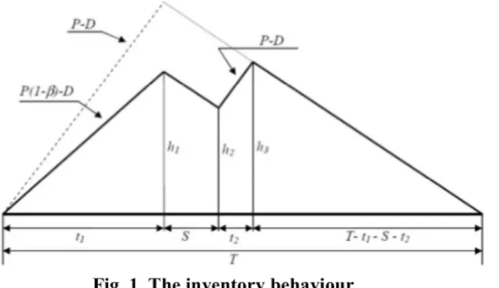
that the %100 inspection operation is performed without time and cost. In other words in order to identify the quality of each product and realize the defective item, each product is inspected after production immediately. Furthermore we assume that each product is perfect or defective. Perfect ones are taken to the warehouse to meet customers’ demands. Demand is continuous with rate per time unit. Defective items are kept in the defective inventory basket next to the machine so that after finishing the production of products and setup time to rework defective items in the same period are reworked. Then all defective items are transformed into perfect and are sent to the warehouse to meet the demands [17]. In Fig.1 the inventory behaviour has been shown in one production period.
Fig. 1. The inventory behaviour.
It has to be mentioned that reworking process is assumed like production process in terms of cost and time. To prevent inventory shortage, not only the production rate must be greater than the demand rate, but also the perfect rate must be greater and the demand rate as follow:
( )
The objective is determining the lot size so that be minimized the sum of discounted cost including present value of setup cost, production (primary production and reworking cost), and machine setup cost to rework the defective products and holding cost.
Assumptions of the model are as follow [11, 17]:
1. It is single product problem. 2. Shortage is not allowable.
3. Inspection cost and time are negligible.
4. Setup operation consumes no time but the cost of every setup is constant. 5. Defective products are reworkable and changeable to perfect ones.
6. The same resources are used for production and reworking and all perfect products are taken to warehouse to meet the demands
9. Demand rate, production time of each product, setup time for re working, percentage of defective item (Exclude costs) are deterministic and constant.
10. Production rate of perfect items is constant and greater than the demand rate of it.
11. Setup time for every rework operation could be nonzero.
12. Reworking in each cycle starts after completion of production operation of each lot immediately.
13. Cost of holding of defective items next to the machines is negligible. 14. Value added is created during production operation.
15. Infinite planning horizon.
3. Determining the Present Value of Total Cost Related to Inventory
in Infinite Horizon
Considering position of product inventory in production cell and warehouse is necessary over the time in order to calculate the types of inventory costs. Since the demand is deterministic, behaviour of product inventory in warehouse approximately is similar to economic production quantity (EPQ) model. Reworking process with considering needed time for reworking is the cause of the difference between presented model and EPQ model. Behaviour of product Inventory level has been shown in Fig. 1. Due to the need to express some points while calculating related to find out the costs and also because of computing the error caused by lack of attention to time value of money, in computation section the Haji’s equations are presented. Equations (1), (2) and (3) show cost function, optimum cycle and optimum lot size respectively.
Annual setup cost for each production period (!"): !"=$%( + ) ='()'+ *
Annual holding cost (! ):
! = , ( + )-$.
Annual cost of the process of production and reworking operation (!/):
!
/= [C (1+θ) Q]+= ( + ) Total annual cost (!+):
!
+ = CD (1+θ) HθDS+('()'*)+ + , ( +
)-$+
.
(1)
Optimum Cycle duration:∗ = 0 ('()'*).
$,.1$1Ө$( )Ө)- (2)
Optimum production amount:
Equations which presented by Haji et al. [1] for production costs including
setup, production and reworking costs: ( + 2)
+ and ( + Ө), show that these two costs are not dependent to lot size, so they are not involved in determining the Cost function and optimum lot size without considering time value money, but as it can be observed in the future, by considering the time value of money, these two costs are effective in calculating the cost function and optimum lot size. Eqs (4), (5) and (6) which could be calculated based on Fig. 1 show how to calculate the time components of each cycle including , 4 and , :
=
%.=
$.(4) where is a constant value
= θ
%.=
$. (5)=
%$(6) As mentioned before, inventory system costs include setup costs (setup to start production and reworking), production cost (primary production and reworking) and holding costs. Moreover it should be noted that during the setup times and reworking, + the systems again incurred setup, production, reworking operation and reworked items holding costs. At first, the present value of one cycle cost iscalculated in order to calculate the present value of sum of planning horizon cost, and then since cycles are the similar, total cost is calculated by Eq. (7) as follow:
= + + + (7)
Now according to the mentioned descriptions and Fig. 1 we proceed to calculating the present value of each cost in each cycle:
3.1. Calculating the present value of setup cost to start production in
each cycle
By probing the Fig. 1 it is illustrated that the constant setup cost for the start of production ( ) which occurred at the beginning of the cycle. So present value of the setup cost to start the production in each cycle is based on Eq. (8):
= (8)
3.2. Calculating the present value of setup cost for reworking
According to the above equation, the present value of setup cost for reworking in each cycle is calculated through Eq. (9):
= <
= 2eρt>
=? @AB1 C '*
D (9)
3.3. Calculating the present value of production cost in each cycle:
According to the notations, production cost per unit of product is unit of currency, and the product could be perfect or imperfect. Since production rate and reworking rate per unit time is unit of product so production or reworking cost is . Then present value of production cost and reworking cost in each cycle is based on Eq. (10).
= < (
(=
cpe
βt) e
αt>
+
<
()) )(
cpe
βt) e
αt>
=
EFG(
e
IJ K
– 1
+
e
G(((LM)JK )N)e
G( JO)N )
)
(10)Calculating the present value of holding cost in each cycle:
Since in notations, holding cost per unit product and amount of inventory in warehouse at time
t
were defined ( ) and ( ) respectively, so inventory holding cost in warehouse in each cycle according to the quantity of inventory at any time is calculated by Eq. (11):Q= < H(t)I(t)=T
>
(11)If ℎ is the holding cost per unit product in unit time and at zero time then ( ) is equal to Eq. (12):
( ) = Vℎ7:W7D = ℎ7D (12)
Based on Eq. (11), in order to holding cost in warehouse, knowing the inventory function according to time is necessary. It could be seen from Fig. 1 that by dividing the period time into the four parts the inventory behavior during entire period could be shown as a function of time. According to the Fig. 1 the inventory behavior as a function of time is as follow Eq. (13):
I(t) X Y Z Y
[,p(,p( θ) D-tθ) D- + ( D)(t ) tϵ, , + s-tϵ,0,
-,p( θ) D- + ( D)(s) + (p D)Vt ( + s)W tϵ, + s, + s +
-,p( θ) D- + ( D)(s) + (p D)( ) + ( D)Vt ( + s + )W tϵ, + s + ,
(13)
By substituting Eqs. (4), (5) and (6) in the Eq. (13) and simplification we have Eq. (14) as follow:
( ) X Z
[Q(,P( θ) Dtθ) D-t tϵ,0, -tϵ, , +
s-θQ ps + (p D)t tϵ, + s, + s +
-Q Dt tϵ, + s + ,
By using the Eqs. (11), (12) and (14) the present value of total cost of holding is based on Eq. (15):
= < I=T
(t)
H (t) >(15)
= e ,(
= (P( θ) D))t-heρt > + e ,
()N
(
Q( θ) Dt -heρt >
+ e() )*, h4 + (h ) -ℎ7D >
()
+ e+ , ->
() )*
= ihℎ; j 7D%( )k)l + m7D%l no + p;47D(%l( )k)) + ;47D(%.)qr
+%D[7@AB(7D )( )- + ; 7@AB,s7D tD%
. + ;4 uv D%
. + -
3.4. Calculating the present value of total costs:
In previous section, each cost of a cycle calculated separately, so total cost of inventory in a cycle according to the Eq. (7) is calculable, meanwhile it is obvious that this cost is repeated similarly in each cycle. Then in order to calculate the present value of sum costs, present values of cost are summed in each cycle according to the present value of money. Since the distance of cycles from each other is equal to the length of each cycle ( ), present value of costs is in Eq. (16) as follow:
( ) = + 7D++ 7 D +…= (1+e1(w1x)Jy +e1 (w1x)Jy +…) (16) If ; = 0 , and the planning horizon is assumed infinite, the expression in parenthesis Eq.(16) would be divergent, then a specific expression cannot be achieved, so to have a convergent total cost function, a finite planning horizon must be considered. But if ; = ≥ 0 (in practice is the same, because at least the interest rate is equal to the inflation rate) the expression in
parenthesis Eq. (16) will be equal to 1 @A{
that in this case, ( ) is converged.
After that by substituting the present value of sum of costs of each cycle ( ) that comes out by using the Eqs. (8), (9), (10) and (15) in the Eq. (16), the present value total cost of inventory is calculated by Eq. (17):
( )
=
{
+
}
?~IJK1 C •
G
€
+
•‚ G
(
e
IJ
K
1+
e
G(JK)ƒJK)„)e
G(JK)„))
+[ FQ G {1 e
IJ((LM)
O +θ(eIJK 1)}+{… ‚(e
IJ
y 1)}+{ ρseG(JK( )ƒ))„)+ρs eG(JK)„)}]
+†Q G[e
IJ
K(eGN1)(1 θ)]+ρ2eIJK[{eGN(G† ‚+ρs 1)}
G†
‚+1] ∗ ( 1 @A{) (17)
8
in the Eq. (17) in addition to = 0 , 2 is also zero. Then it can be seen when = 0 the Eq. (17) will result the same equation of the present value of total costs,
= =
‡ = 0 , 2 Cm= •‚ρ(eρ(
J((Lθ)
K ) )
ℎ= ‚Q ρ[(1 e
Jρ((Lθ) K +θ (eJ
ρ
K 1)) + … ‚(e
Jρ
y )-
As it can be seen, costs , and have changed, consequently we have:
( ) ={A+ ˆ.D(7D(A((L‰)B )1) + .D[(1 7A@((L‰)B +θ (7A@B 1)) + $.(7A@{ 1)]}m
1@A{n
5. Methodology of Solving the Problem
Equation (17) is a single variable function of . If its second derivative is positive, this function is always convex and has absolute minimum points. To find optimum point the function should be derived of and its root should be found. Calculations show that the result of first and second derivative is complicated and too long. Studies show that calculating the root of first derivative as the optimum point and showing the positivity of second derivative are impossible. Also using the linear approximation 71Š= ‹ +Š^ does not solve the problem because calculations show the complexity of the derivation of function remains by using this approximation. According to the inefficiency of derivative technique in calculating the roots of function search methods should be considered. Most of the numerical optimization methods are based on producing series of approximate values as according to its values, function is improved. In this article the combination of search algorithm with accelerated motion (in order to quick search through an interval in which solution exist, and dichotomous method (in order to reduce selected interval and introducing a point near to the optimum point) has been used [26] This combination is able to close to the optimum solution with any desired accuracy. In aforementioned method, the • Ž is used as initial starting point. Steps of this algorithm are as follow (in this algorithm ‹is the accuracy and
•
is a small number):Step 0: Consider the single variable function ( ) Step1: determine the initial start point
( =), ( == • Ž). If ( =+ •) ( =), set 4 = 0.02 = otherwise set 4 = 0.02 =.
Step2: set = = . As long as ( ) < ( =) set = + . Step3: if = , values replace =and with each other.
Step4: set =∗= =+ ( =)/2 ‹/2 and ∗= =+ ( =)/2 + ‹/2
•
If
(
=∗) <
(
∗)
then remove
∗and set:
=
∗.
• If ( =∗) = ( ∗) select two other points as =and . (by change in ‹).
Step5
: if
“ (
=∗)
(
∗)“ < ‹
then set:
∗= (
=∗+
∗)/2
. (
∗is
close to the optimum solution of Eq. (16). Otherwise go to step4.
6. Numerical Example
In this section by expressing a numerical example, the results of the proposed model are compared with the results of the Haji’s model.
According to the [11, 17] the following numerical example is given:
=1900 $/order = 100 product unit/year 2= 1100 $/order = 120 product unit/year = 1100 product unit /year ℎ= 6 rial/year. Product unit = 1 day = %17
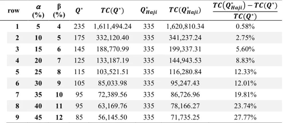
Table 1 shows the approximate solution of this example with present value of total costs which is calculated by Eq. (3). In this table, nine different values of interest rate and inflation rate have been considered.
Table 1. Solving a numerical example for different values of interest rate and inflation rate and comparing with Haji’s model.
row αααα (%)
β
(%) ”∗ •–(”∗) ”—˜™š
∗ •–(”
—˜™š
∗ ) •–V”—˜™š∗ W •–(”∗) •–(”∗)
1 5 4 235 1,611,494.24 335 1,620,810.34 0.58 %
2 10 5 175 332,120.40 335 341,237.24 2.75 %
3 15 6 145 188,770.99 335 199,337.31 5.60 %
4 20 7 125 133,187.19 335 144,943.53 8.83 %
5 25 8 115 103,521.51 335 116,280.84 12.33 %
6 30 9 105 85,033.98 335 95,247.43 12.01 %
7 35 10 95 72,389.56 335 86,726.96 19.81 %
8 40 11 95 63,169.76 335 78,166.27 23.74 %
9 45 12 85 56,145.50 335 71,735.25 27.77 %
5
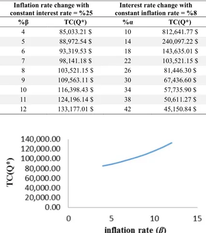
Table 2. Changes trend of optimum value of total costs is shown for changes of interest rate and inflation rate.
Inflation rate change with constant interest rate = %25
Interest rate change with constant inflation rate = %8
%β TC(Q*) %α TC(Q*)
4 85,033.21 $ 10 812,641.77 $
5 88,972.54 $ 14 240,097.22 $
6 93,319.53 $ 18 143,635.01 $
7 98,141.18 $ 22 103,521.15 $
8 103,521.15 $ 26 81,446.30 $
9 109,563.11 $ 30 67,436.60 $
10 116,398.43 $ 34 57,735.90 $
11 124,196.14 $ 38 50,611.27 $
12 133,177.01 $ 42 45,150.84 $
Fig. 2. Total cost changes trend compared to inflation rate (α = %25).
6
7. Conclusion:
In this study the effect of time value of money and inflation rate on an inventory model have been explored with considering reworking defective items whilst shortage of inventory is not allowed for single product case.
• The cost function has been obtained by considering time value of money and inflation rate on costs (setup for starting the production, setup for reworking, reworking, production and holding) and at the end summation these costs after giving effect of interest rates and inflations.
• The optimum quantity of each cycle has been computed by drawing (inventory total cost) chart at the point that the cost function is minimized.
• Also effect of time value of money and inflation rate (efficiency of model) has been considered by using a numerical example.
For future research some cases can be suggested such as:
• Solving the model in finite time horizon, solving for random number of defective items or random rate for producing defective rate, developing the model with reworking the outputs, solving the model for multi product case, developing the model for the case of using different resources for production and reworking.
References
1. Hadley, G. (1964). A Comparison of Order Quantities Computed using the Average Annual Cost and the Discounted Cost. Management Science, 10(3), 472 476.
2. Porteus, E.L. (1986). Optimal Lot Sizing Process Quality Improvement and Setup Cost Reduction. Operations Research, 34(1): 137 144.
3. Rosenblat, M.J.; and Lee, H.L. (1986). Economic Production Cycles with Imperfect Production Processes. IIE Transactions, 18(1): 48 55.
4. Moon, I.; and Lee, S. (2000). The effects of inflation and time value of money on an economic order quantity model with a random product life cycle. European Journal of Operational Research, 125(3):588 601.
5. Salameh, M.K.; Jaber, M.Y., (2000). Economic production quantity model for items with imperfect quality. International Journal of Production Economics, 64(1 3):59 64.
6. Cárdenas Barrón, L.E. (2000). Observation on: “Economic production quantity model for items with imperfect quality” [Int. J. Production Economics 64 (2000) 59–64]. International Journal of Production Economics, 67(2):201.
7. Goyal, S.K.; and Cárdenas Barrón, L.E. (2002). Note on: Economic production quantity model for items with imperfect quality – a practical approach. International Journal of Production Economics, 77(1):85 87. 8. Chan, W.M., Ibrahim, R.N., Lochert, P.B. A., 2003. New EPQ Model:
7
9. Flapper, SDP.; and Jensen, T. (2004). Logistic Planning of Rework with Deteriorating Work in Process. International Journal of Production Economics, 88(1): 51 59.
10. Jamal, A.M.M.; Sarker, B.R.; and Mondal, S. (2004). Optimal Manufacturing Batch Size with Rework Process at a Single Tage Production System. Computers & Industrial Engineering, 47(1): 77 89.
11. Haji, A.; Haji, R.; and Bijari, M. (2006). The Newsboy Problem with Random Defective and Probabilistic Initial Inventory. Proceeding of the 36th CIE Conference on Computers & Industrial Engineering, Taipei, Taiwan 3498 3502.
12. Tsou, J.C. (2007). Economic Order Quantity Model and Taguchi.s Cost of Poor Quality. Applied Mathematical Modelling, 31(2): 283 291.
13. Lo, Sh.T.; Wee, H.M.; and Huang, W.C. (2007). An integrated production inventory model with imperfect production processes and Weibull distribution deterioration under inflation. International Journal of Production Economics, 106(1): 248 260.
14. Kumar Dey, J.; Mondal, S.K.; Maiti, M. (2008). Two Storage Inventory Problem with Dynamic Demand and Interval Valued Lead Time over Finit Time Horizon Under Inflation and Time Value of Money. European Journal of Operational Research, 185(1):170 194.
15. Mirzazadeh, A. (2010). Effects of Variable Inflationary Conditions on an Inventory Model with Inflation Proportional Demand Rate. Journal of applied science, 10(7): 551 557.
16. Bayati , F.; Rasti , B.M.; and Hejazi , M.S.R. (2011). A Joint Lot Sizing and Marketing Model with Reworks, Scraps and Imperfect Products Considerations. International Journal of Industrial Engineering Computations, 2(2):395 408.
17. Moslehi. G.; Rasti B. M.; and Bayati. F.M. (2011). The Effect of Inflation and Time Value of Money on Lot Sizing By Considering of Rework in an Inventory Control Model. International Journal of Industrial Engineering & Production Management, 22(2):181 192.
18. Fathi Hafshejani, K.; Valmohammadi, V.; and Khakpoor, A. (2012). Retracted: Using genetic algorithm approach to solve a multi product EPQ model with defective items, rework, and constrained space. Journal of Industrial Engineering International, 8(27).
19. Taheri Tolgari, J.; Mirzazadeh, A.; and Jolai,F. (2012). An inventory model for imperfect items under inflationary conditions with considering inspection errors. Computers & Mathematics with Applications, 63(6): 1007 1019. 20. Alfares, H. (2012). An EPQ Production Inventory Model with Variable
Holding Cost. International Journal of Industrial Engineering: Theory, Applications and Practice, 19(5).
21. Mondal, M.; Maity, A.K.; and Maiti, M. (2013). A production repairing inventory model with fuzzy rough coefficients under inflation and time value of money. Applied Mathematical Modelling, 37(5): 3200 3215. 22. Taleizadeh, A.A.; Cárdenas Barrón, L.E.; and Mohammadi, B., (2014). A
scraped products, rework and interruption in manufacturing process. International Journal of Production Economics, 150(April 2014):9 27. 23. Majumder, P.; Bera, U.K.; and Maiti, M. (2014). An EPQ model for a
deteriorating item with inflation reduced selling price and demand with immediate part payment. HACETTEPE JOURNAL OF MATHEMATICS AND STATISTICS, 43(4), 641 659.
24. Li, N.; Chan, F. T.; Chung, S. H.; and Tai, A. H. (2015). An EPQ Model for Deteriorating Production System and Items with Rework. Mathematical Problems in Engineering, (2015).
25. Sarkar, B.; Sana, S.S.; and Chaudhuri, K. (2011). An imperfect production process for time varying demand with inflation and time value of money – An EMQ model. Expert Systems with Applications, 38(11): 13543 13548. 26. Chung, K.J.; Lin, S.D.; Chu, P.; and Lan, S.P. (1998) .The Production and