Entropy production and multiple equilibria: the case of the ice-albedo feedback

www.earth-syst-dynam.net/2/13/2011/ doi:10.5194/esd-2-13-2011

© Author(s) 2011. CC Attribution 3.0 License.

Earth System

Dynamics

Entropy production and multiple equilibria:

the case of the ice-albedo feedback

C. Herbert1,2, D. Paillard1, and B. Dubrulle2

1_{Laboratoire des Sciences du Climat et de l’Environnement, IPSL, CEA-CNRS-UVSQ, UMR 8212, Gif-sur-Yvette, France} 2_{Service de Physique de l’Etat Condens´e, DSM, CEA Saclay, CNRS URA 2464, Gif-sur-Yvette, France}

Received: 5 October 2010 – Published in Earth Syst. Dynam. Discuss.: 19 October 2010 Revised: 24 January 2011 – Accepted: 2 February 2011 – Published: 23 February 2011

Abstract. Nonlinear feedbacks in the Earth System pro-vide mechanisms that can prove very useful in understand-ing complex dynamics with relatively simple concepts. For example, the temperature and the ice cover of the planet are linked in a positive feedback which gives birth to multiple equilibria for some values of the solar constant: fully ice-covered Earth, ice-free Earth and an intermediate unstable solution. In this study, we show an analogy between a classi-cal dynamiclassi-cal system approach to this problem and a Maxi-mum Entropy Production (MEP) principle view, and we sug-gest a glimpse on how to reconcile MEP with the time evo-lution of a variable. It enables us in particular to resolve the question of the stability of the entropy production maxima. We also compare the surface heat flux obtained with MEP and with the bulk-aerodynamic formula.

1 Introduction

A very broad class of problems in climate modelling con-sists of studying the evolution of a particular field (e.g. sur-face temperature, precipitation,etc) when an external param-eter, orforcing, is varied. Most of the time, the response to this variation is not linear. Feedbacks can amplify or damp the effect of the initial perturbation. One of these feedbacks aroused a proficient branch in scientific literature in the 70s’, when Budyko and Sellers simultaneously suggested that the interaction between sea ice and climate could have dramatic consequences. Indeed, the higher the global temperature on Earth, the less the ice cover is likely to extend, and thus the lower the albedo. A lower albedo leads in turn to a higher global temperature, and so on and so forth until all the ice is melted. Stimulated by this pioneer work, the questions

Correspondence to:C. Herbert (corentin.herbert@lsce.ipsl.fr)

of the stability of the climate as well as the consequences such feedbacks might have for understanding paleoclimates were extensively studied, using the whole hierarchy of mod-els, from the most simple Energy Balance Models (EBMs) to the complex General Circulation Models (GCMs).

Using 1D EBMs, Budyko and Sellers had found two stable equilibrium positions for the edge of the ice cover, one corre-sponding to the present climate and one to a fully ice-covered Earth (Budyko, 1969; Sellers, 1969). A large part of the subsequent work was concerned with verifying that these re-sults still held with various different versions of the Budyko-Sellers models, with different heat transport parameteriza-tions, temperature dependance expressions in the planetary albedo, numerical schemes,... (Faegre, 1972; Schneider and Chen, 1973; Held and Suarez, 1974; North, 1975a; Gal-Chen and Schneider, 1976, e.g.). Some elegant analytical solutions were found for these models (Chylek and Coak-ley, 1975; North, 1975a,b), and various mathematical meth-ods were applied to determine the stability of the equilibria (Ghil, 1976; Su and Hsieh, 1976; Frederiksen, 1976; Cahalan and North, 1979; North et al., 1979). Owing to the extreme sensitivity of climate to variations in the solar constant found by the first studies, the precise position of the tipping point between present climate and adeep freezedEarth was of pri-mary concern. Further investigation by Lian and Cess (1977) and Oerlemans and van den Dool (1978) revealed that the sensitivity was much less than initially thought. A fundamen-tal question raised by these results was that of thetransitivity

of the climate system in Lorenz’s terminology (Lorenz, 1968, 1970), and the difference between forced and free fluctua-tions (Schneider and Gal-Chen, 1973; Ghil, 1976; Fraedrich, 1978). For a comprehensive review of the various models, parameterizations and problems pertaining to Energy Bal-ance Models and the ice-albedo feedback, the reader is re-ferred to North et al. (1981).

dynamical system theory: how do multiple equilibria arise from the ice-albedo feedback, what does the bifurcation dia-gram look like, etc. The model used here is a two box energy balance model with a simplified radiative transfer using the

Net Exchange Formulation(see e.g. Dufresne et al., 2005), and a bulk aerodynamic formula for the surface heat flux. In a second step, we draw an analogy between this dynamical system view and the results obtained when predicting the sur-face heat flux from the Maximum Entropy Production (MEP) principle. The MEP principle, as originally expressed by Pal-tridge (1975, 1978, 1979) for the climate system, provides a variational principle to compute energy fluxes that are not otherwise constrained by the laws of physics. Originally, Paltridge and others applied MEP to the meridional energy transport (Paltridge, 1975, 1978; Grassl, 1981; Gerard et al., 1990; Lorenz et al., 2001, e.g.), but other studies (Ozawa and Ohmura, 1997; Pujol and Fort, 2002) indicate that it may be valid on the vertical also.

As noticed by Oerlemans and van den Dool (1978), Crafo-ord and K¨all´en (1978) and Fraedrich (1978), the bifurca-tion giving birth to multiple equilibria in the case of the ice-albedo feedback has a fundamentally radiative nature, and has nothing to do with transport properties of the atmosphere. This encourages one in thinking that a zero-dimensionnal model is sufficient to capture the structure of the mecha-nism while avoiding the use of more cumbersome mathe-matics (namely the Sturm-Liouville theory, required for one-dimensional models such as Ghil, 1976). Therefore we will restrict ourselves here to this idealized case. Note also that most of our work could be transposed easily to other feed-backs, like the water-vapour feedback.

2 The ice-albedo feedback, multiple equilibria and the hysteresis cycle: the dynamical system approach

2.1 A simple two-layer EBM using the net exchange formulation

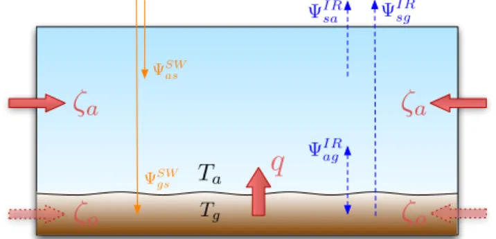
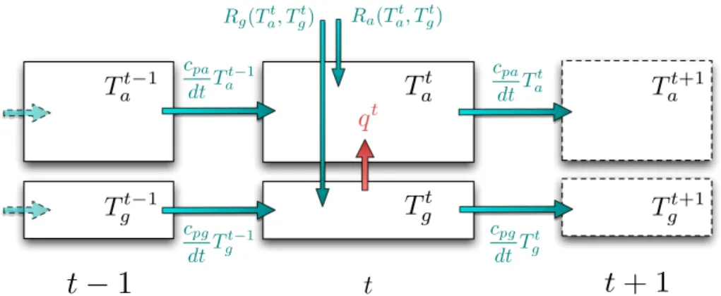
We use a slightly different formulation of the model de-scribed in Herbert et al. (2010), as represented in Fig. 1. A grid cell is characterized by a surface temperatureTgand an

atmospheric temperatureTa, and we note9gsSW(respectively

9_asSW) the flux of solar energy received by the ground (re-spectively absorbed by the atmosphere). Radiative exchange use theNet Exchange Formulation, in which the basic objects are not energy fluxes at a given level but rather the energy ex-change rate between two layers in the atmosphere or between one layer and a boundary surface (see Dufresne et al., 2005). 9_agIRis the net energy exchange rate between the ground and the atmospheric column per unit surface (i.e. the greenhouse effect), and9_saIR (respectively9_sgIR) is the cooling to space term for the atmosphere (respectively the surface). The net

ΨSW as

ΨIR sg

ΨIR sa

ΨIRag

T

Tg

q

gs

ζ

ζ

ζ

ζo

Fig. 1.A grid cell of the model, adapted from Herbert et al. (2010).

9_ijν are the energy exchange rates per unit surface due to radiative transfer (see text),qis the surface heat flux andζais the atmospheric

energy convergence. Over the oceans, there is also an oceanic en-ergy convergenceζo.

energy exchange rates per unit surface are expressed as func-tions ofTgandTaas:

9_gsSW = (s(α)¯ −s)(1 −α) ξ S, (1)

9_asSW = s +α s∗ξ S, (2)

9_agIR = t σ T_g4 −t σ T_a4, (3)

9_saIR = t σ T_a4, (4)

9_sgIR =

1− t µ

σ T_g4, (5)

whereσ is the Stefan-Boltzmann constant,αis the surface albedo,t, s, s∗, s¯ are radiative coefficients, S is the solar constant,ξ accounts for the annual mean zenith angle of the sun andµis the Elsasser factor (see Herbert et al., 2010 for a derivation of the equations and a discussion of the coeffi-cients).

In addition to radiation, energy is exchanged due to atmo-spheric and oceanic transport as well as surface heat fluxes. Let us merge all these energy transfer modes into two vari-ables: γa (respectivelyγg) represents the net convergence

(the opposite of the divergence) of energy into the atmo-spheric cell (respectively the surface layer). Writingζa for

the atmospheric convergence (this variable was designated byζ in Herbert et al., 2010),ζofor the oceanic convergence

(this was not taken into account in Herbert et al., 2010), and qfor the surface heat flux, we have

γa = ζa +q, (6)

γg = ζo −q. (7)

fluxes, atmospheric transport, and oceanic transport when ap-plicable. Of course, over land, it is reasonable to assume thatγgis just the surface energy flux (i.e.ζo= 0) , and then

γa+γgis the convergence of energy due to the atmospheric

flow. In this study, as we will only use the zero-dimensional version of this model, we will always haveζa=ζo= 0, and

thusγa=−γg= q.

At steady-state, the energy balance equations for the atmo-sphere and the surface read

Ra Ta, Tg +γa = 0, (8)

Rg Ta, Tg +γg =0, (9)

where

Ra Ta, Tg =9asSW +9agIR −9saIR (10) = s +α s∗ξ S +t σ T_g4 −₂σ T_a4,

Rg Ta, Tg = 9gsSW −9agIR −9sgIR (11) = (s¯ −s)(1 −α) ξ S −t σ T_g4 −σ T_a4

−

1 − t µ

σ T_g4.

In this form, the steady-state Eqs. (8)–(9) cannot be solved sinceγaandγgare unkown. In the next section we introduce

a parameterization of these quantities as functions ofTaand

Tg. In Sect. 3, we use the MEP principle to compute them.

2.2 The zero-dimensional model with bulk aerodynamic formula

In the case of a zero-dimensional, two-layer model consid-ered here, the net convergence of energy in the atmospheric box (i.e. the divergence of the diabatic heating at the surface, γa=q=−γg) can be simply interpreted as the surface heat

flux. In this section, we adopt a bulk aerodynamic formula (Peixoto and Oort, 1992) to express this flux as a function of the temperaturesTaandTg:

γa = qbaf Ta, Tg = cpaCDus Tg −Ta. (12)

whereCDis the drag coefficient,usis the surface wind speed

andcpais the heat capacity of the atmosphere per unit surface

area (similarlycpg is the heat capacity of the ground). Now

the model can be seen as a two-dimensional dynamical sys-tem:

_˙

Ta ˙ Tg

=F Ta, Tg, (13)

with F Ta, Tg

=

F1 Ta, Tg

F2 Ta, Tg

, (14)

and

F1 Ta, Tg =

1 cpa

Ra Ta, Tg + qbaf Ta, Tg, (15)

F2 Ta, Tg =

1 cpg

Rg Ta, Tg −qbaf Ta, Tg. (16)

Our main interest here is to find the equilibrium positions of the system, i.e. the fixed points of the dynamical system, given by the roots of F, and to study their stability. Of course, the dynamics of a two-dimensional dynamical sys-tem can be more complex than just a relaxation to an equi-librium position (although it is still rather gentle, see Guck-enheimer and Holmes, 1983 for example), contrary to one-dimensional dynamical systems. Still, let us note here that the first equation inF (Ta, Tg)= 0 can be solved algebraically

inTa to obtain a relation Ta∗=f (T ∗

g)where(T ∗ a, T

∗ g)is a

fixed point of the system. Thus the number of fixed points of the two-dimensional system is exactly the number of roots of the scalar equationF2(f (Tg), Tg)= 0.

For simplicity, we will consider here the projection of the dynamical system (Eq. 13) onto theTgaxis:

˙

Tg = F2 f Tg, Tg. (17)

As just explained, this dynamical system, although not mathematically equivalent to the full dynamical system (Eq. 14), has the same equilibrium positions. Physically, this simplification is motivated by the fact that the atmosphere can be assumed to reach equilibrium very quickly, hence the evolution ofTa is enslaved by the dynamics ofTg. In other

words, the system (Eq. 17) is just the system (Eq. 14) with cpa= 0.

2.3 Multiple equilibria

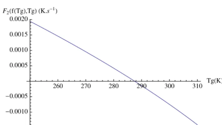
The values of the coefficients used here are reproduced in Table 1. Taking for the albedo the fixed value α0= 0.15,

the system only has one fixed point, as plotting the function F2(f (Tg), Tg)= 0 clearly shows (see Fig. 2). In this case,

the equilibrium is at a global mean surface temperature of T_g0≈288 K.

But in reality, the higher the global mean temperature, the lower the extent of the regions that can sustain an ice-cover. This positive feedback can be encoded in the following tem-perature dependance for the albedo:

α Tg = αF +

(αI −αF)

2

1 +tanh

_T 0 −Tg

1T

,(18) whereαF(respectivelyαI) represents the value of the

plan-etary albedo over an ice-free (respectively fully ice-covered) area, andT0and1T are parameters determining the

Table 1.Values for the parameters of the 0D model (radiative coefficients, bulk aerodynamic formula parameters and ice-albedo feedback parameterization). Note that the values for the heat capacities depend on the thickness of the layer and on the nature of the surface (ocean or land), but this has no influence on the steady-state results.

Symbol µ ξ t s s∗ s¯ α₀ S₀

Value 0.6 0.25 0.44 0.19 0.015 0.89 0.15 1368 W m−2

Symbol CD us cpa cpg αI αF T0 1T

Value 0.008 6 m s−1 1 MJ K−1m−2 210 MJ K−1m−2 0.08 0.68 273.15 K 15 K

260 270 280 290 300 310 TgHKL

-_0.0010 -_0.0005

0.0005 0.0010 0.0015 0.0020

F2HfHTgL,TgL HK.s

-1_L

Fig. 2.FunctionF2(f (Tg), Tg)as a function ofTg(see text) with

a fixed albedo has only one root.

choose this expression because it depends smoothly on the temperature.

Replacingαin Eq. (14) with Eq. (18) yields a new dynam-ical system

_˙

Ta ˙ Tg

=G Ta, Tg, (19)

where the fixed points are again determined by the condi-tions,gbeing defined similarly tof (or obtained by substi-tution of the albedo function intof),

T_a∗ =gT_g∗, (20)

0 = G2

gT_g∗, T_g∗. (21)

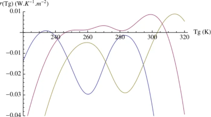
Plotting the curve G2(g(Tg), Tg) as a function of Tg

(Fig. 4) shows that for certain values of the solar constant, three solutions coexist. This range can be determined to be approximately 0.98S0≤S≤1.08S0. Outside this range,

only one solution subsists. For the present value of the solar constant,S=S0, for instance, these equilibria correspond to a

fully glaciated Earth (snowballstate)T_gS≈249 K, an ice-free EarthT_gP≈287 K which can be identified with the present climate, and an intermediate glacial stateT_gG≈275 K. For a low value of the solar constant (e.g. 0.95S0), only the

snowball stateT_gS subsists. Similarly, at high solar constant

240 260 280 300 TgHKL

0.2 0.4 0.6 0.8 1.0

ΑHTgL

Fig. 3.Surface albedoαas a function of surface temperatureTgin

K.

250 260 270 280 290 300 310 TgHKL

-_0.0010 -_0.0005

0.0005

G2HgHTgL,TgL HK.s

-1_L

Fig. 4. FunctionG₂(g(Tg), Tg)as a function ofTg(see text)

in-cluding the ice-albedo feedback for different values of the solar constant: 0.95S0(blue),S0(red), 1.05S0(yellow), 1.1S0(green).

(e.g. 1.1S0), the only equilibrium is found on the ice-free

branchT_gP.

0.9 1.0 1.1 1.2

S

S0

-₄₀ -30 -₂₀ -10

10 20 30 TgH°CL

Fig. 5. Bifurcation diagram of the bulk aerodynamic formula model. TG, TP andTS are plotted againstS/S0when they exist.

Stable fixed points are plotted in blue while the unstable solution is in dotted red. This figure clearly shows that two saddle-node bifur-cations occur at respectivelyS≈0.98S0andS≈1.08S0.

The stability can also be read directly on Fig. 4 for the 1D-reduced system: stable equilibria correspond to roots of the function with negative derivative, while at the unstable equi-librium, the curve crosses the x-axis with an upward slope.

Summarizing the above results, Fig. 5 represents the curve of the fixed points when sweeping a large range of values forS: it is the bifurcation diagram of the dynamical system. Creation of a pair of stable/unstable equilibria at the tipping points 0.98S0 and 1.08S0 is called a saddle-node bifurca-tion. Thus the hysteresis curve obtained for the temperature stems from the bifurcation structure of the dynamical system as two back-to-back saddle-node bifurcations. It is notewor-thy that this figure does not depend upon the particular coficients choice in the bulk formula, nor on the greenhouse ef-fect. Would we setqbaf= 0 (radiative equilibrium with

green-house effect) or/andt= 0 (greenhouse effect shut down), the hysteresis curve would remain qualitatively the same. 2.4 Potential for the dynamical system

The full two-variables dynamical system (Eq. 13) cannot be expressed as the gradient of a potential function, but its one-dimensional projection can, like any other one-one-dimensional dynamical system. Let us thus introduce the potentialV (de-fined up to an additive constant) such that

˙ Tg = −

∂V ∂Tg

. (22)

Fixed points of the dynamical system correspond to criti-cal points (i.e. extrema in this 1-D case) of the potential. The stability criterion becomes that stable fixed points are min-ima of the potential:

−∂ 2_V

∂T2 g

<0, (23)

while its maxima are unstable fixed points.

240 260 280 300 320 TgHKL

0.1 0.2 0.3 0.4 0.5 0.6 0.7

VV0

Fig. 6.PotentialV (normalized) as a function of temperatureTg(in

K) for three different values of the solar constant: 0.95S0(red),S0

(blue) and 1.1S0(yellow). For the present value of the solar

con-stant, the potential has a double well shape, with two stable equi-libria, while for the two other values, the potential has only one minimum.

Figure 6 shows the shape of the potential for different val-ues of the solar constant. At low solar constant (e.g. 0.95S0),

the potential has only one critical point, a minimum at T≈_{245 K. Increasing the value of the solar constant levels} down the potential curve, until a second local minimum ap-pears (along with a local maximum) withT above the freez-ing point, aroundS≈0.98S0. AtS=S0, it is clear that the

potential has two minima atT ≈250 K andT ≈290 K and a maximum atT ≈275 K. Further increase of the solar con-stant leads to a deeper minimum atT >0◦C while the min-imum atT <0◦C becomes shallower. AroundS≈1.08S0,

the minimum atT <0◦C disappears (it annihilates with the local maximum); forS= 1.1S0, the only minimum is found

atT ≈300 K.

Note that, as expected, the critical points of the potential obtained for the three values of the solar constant consid-ered here match with the values of Fig. 4. Also, the number of critical points of the potential changes at the bifurcation points of the dynamical system.

3 The entropy production rate and the ice-albedo feedback

In this section, we do not use anymore the bulk aerody-namic formula for the surface fluxγa=−γg, but the

270 280 290 300 310 320 TgHKL

-_0.10 -0.08 -0.06 -_0.04 -_0.02 ΣHTgL HW.K-1

.m-2_L

Fig. 7. Entropy production rate as a function of the surface tem-peratureTgfor the 0D model atS=S0. The only local maximum

corresponds toTg≈295 K.

the comments in Grinstein and Linsker, 2007; Bruers, 2007). More details on theoretical issues and practical use can be found in Ozawa et al. (2003); Kleidon and Lorenz (2005); Martyushev and Seleznev (2006).

3.1 The entropy production rate in zero-dimensions

Let us consider the model of Sect. 2.1 and introduce the en-tropy production rate per unit surface

σ = γa Ta

+ γg Tg

. (24)

Substituting Eqs. (8)–(9) into Eq. (24) forγaandγg,σcan

be considered as a functional of the temperature field. We are looking for its maxima subject to the constraint

γa +γg = 0. (25)

The sum of Eqs. (8) and (9) can thus be solved forTaas a

function ofTg, and the entropy production rateσis simply a

function of one variable. Its graphical representation for the set of parameters given in Table 1 (fixed albedoα0) is shown

in Fig. 7. It is clear that there is only one local maximum, corresponding to a surface temperatureTg≈295 K.

Now, replacing in the equations the constant albedoα0by

the temperature-dependent albedo (Eq. 18), the resulting en-tropy production rate curve is plotted in Fig. 8 for different values of the solar constant.

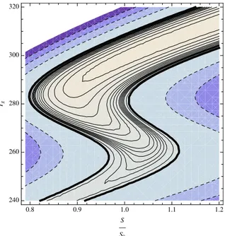
Unlike the potential for the dynamical system in Sect. 2.4, the entropy production rate always has at least two local max-ima and a local minimum. In fact, over a rather narrow range, estimated to be 0.95S0≤S≤1.005S0, the entropy

produc-tion rate even has three maxima and two minima. This is even clearer on the contour plot of the entropy production rate as a function ofTgandS/S0(Fig. 9). Hence, there is

indeed an analogue of thefold of the potential in the clas-sical dynamical system picture in the context of the entropy production surface, but the values at which it takes place do not exactly correspond.

240 260 280 300 320 TgHKL

-_0.04 -0.03 -_0.02 -_0.01

0.01

ΣHTgL HW.K-1

.m-2_L

Fig. 8. Entropy production rate as a function of the surface tem-peratureTgfor the 0D model with ice-albedo feedback. For a low

value of the solar constant (S= 0.8S0, blue curve), there is only one

local maximum with positive entropy production rate. The same holds for high solar constant (S= 1.2S0, yellow curve), while there

are three local maxima and two minima, all with positive entropy production rates, forS=S0(red curve).

Besides, a large portion of the curve on Fig. 8 lies under the abscissa axis: for the corresponding range of tempera-ture values, the entropy production rate is negative, contrary to what the second law of thermodynamics states (or more precisely its extension to non-equilibrium systems). It seems reasonable to impose the condition

σ Tg ≥ 0, (26)

thereby restricting the range of valuesTgcan actually take. In

this case, this is equivalent to requiring that the surface heat flux goes from hot to cold. With this additional constraint, the range of possible values of the solar constant allowing for coexistence of multiple equilibria (two or three) can be determined approximately: 0.8S0≤S≤1.12S0.

3.2 Stability of the MEP states

0.8 0.9 1.0 1.1 1.2 240

260 280 300 320

S

S0

Tg

Fig. 9. Contour plot of the entropy production rate as a function of the solar constant (normalized by its present-day value) and the surface temperatureTg(in K). Negative contour lines are dashed,

positive contour lines are solid and the null contour line is the thick solid line. Shades of blue represent negative values of the entropy production rate.

find a practical way to select a local maximum for given ini-tial conditions. As a particular case, we would obtain a way to distinguish between local entropy production maxima rep-resentingdynamically stablesteady-states and dynamically unstableones.

This involves the introduction of time in the MEP formu-lation. So far, there was no mention of time in the MEP ap-proach as we were only concerned with steady-states. Even though we claim that the entropy production maxima cor-respond to equilibrium points,−σ is by no means a poten-tial for the dynamical system. Indeed, the dynamics of the system is simply given by the first law of thermodynamics. Here, it reads

cpa

dTa

dt = Ra Ta, Tg

+γa, (27)

cpg

dTg

dt = Rg Ta, Tg

+γg. (28)

Similarly to the steady-state entropy production rate, we can define the instantaneous entropy production rate: σi(t ) =

γa(t )

Ta(t )

+ γg(t ) Tg(t )

(29)

= 1

Ta(t )

cpa

dTa

dt −Ra Ta, Tg

+ 1

Tg(t )

cpg

dTg

dt − Rg Ta, Tg

using Eqs. (27)–(28). Note that the instantaneous entropy production rate σi and the steady-state entropy production

rateσ coincide at steady-state.

Asσiappears as the natural generalization ofσtaking into

account the time derivative of the dynamical variables, we suggest that the system may follow the trajectory maximizing the instantaneous entropy production rate, seen as a function of the time-dependent unknown fluxesγa,γg(always linked

by the relationγa+γg= 0). This approach is very similar to

what Jaynes (1980) advocates for.

In practice, it is easier to reformulate the above suggestion with a time-discretized system (see Fig. 10). Let us consider two snapshots of the system separated by a finite time in-tervaldt. We note T_at, T_gt the values of the air and surface temperature at timet. The instantaneous entropy production rate becomes:

σ_it = 1 Tt

a

cpa

T_at −T_at−1 dt −Ra

T_at, T_gt

!

(30)

+ 1 Tt g

cpg

T_gt −T_gt−1 dt −Rg

T_at, T_gt

!

Suppose we know the state of the system at time t−1 (i.e. T_at−1 andT_gt−1are given). Then our postulate is that T_at andT_gt can be chosen so as to maximizeσ_it (with fixed T_at−1andT_gt−1) subject to the constraintγ_at+γ_gt= 0. Iterat-ing this process leads to a trajectory maximizIterat-ing the instanta-neous entropy production rate at each timestep, starting from a given initial condition.

Integrating the system with this method, initialized in the vicinity of the different maxima of the entropy production rate at steady-state, provides a criterion for stability: it is found here that the warm branch as well as the snowball branch of Fig. 9 are stable, while the intermediate branch is unstable. The maxima of the entropy production and their stability are plotted as functions of the solar constant on Fig. 11, analogously to Fig. 5. This result draws the final line in the parallel between the dynamical system approach and the MEP approach. Note that the limits of this analogy are reached at some points: Fig. 11 cannot be considered as a usual bifurcation diagram. As a consequence, the lines of ex-istence of the maxima need not depend continuously on the parameter, and for certain values of the parameter (for exam-pleS≈0.9S0), two stable maxima coexist with nounstable manifoldto separate them.

T

a

T

t a

T

T

g

q

cpa

dtT

t−1

a

cpg

dtT

t−1

g

t

₋

1

t

Rg(Tat, T t

g) Ra(Tat, Tgt)

T

T

t

+ 1

cpa

dtT

t a

cpg

dtT

t g

Fig. 10.To discuss the stability of the steady states predicted by MEP, we need to extend the principle to obtain a time-dependent formulation. This is done by maximizing the instantaneous entropy production rate. To compute the time derivative of the temperature, we consider it as a known flux in time seen as a geometric dimension of the space upon which MEP operates (see text). In green, the fluxes that can be computed from the state variables(Tat−1, Tat, Tt

−1

g , Tgt). In red, the unknown flux obeying MEP.

0.7 0.8 0.9 1.0 1.1 1.2 1.3

S

S0

220 240 260 280 300 320

TgHKL

Fig. 11.Entropy Production maxima as a function of the solar con-stant, normalized by its present value. The solid lines (respectively the dotted line) correspond to dynamically stable (respectively un-stable) equilibria in the sense of Sect. 3.2. Note that this is not a bifurcation diagram in the usual meaning.

valuable to investigate the range of validity of this new appli-cation of the MEP principle in future studies, theoretically or on other examples. We can already adduce some mate-rial to support ourrelaxation equationsapproach. In fact, the only novelty as compared to the common use of MEP in the steady-state context is the inclusion of time derivatives of the dynamical variables in the entropy production rate. But one can simply consider these time derivatives as known fluxes, playing exactly the same role asRa(Ta, Tg)orRg(Ta, Tg).

The only difference is that computing these fluxes requires that we consider a bigger system (here simply the state of the system at timest−1 andt), even though the number of unknowns in the big system remains the same (Tat andTgt,

whereasT_at−1andT_gt−1are fixed). In this respect, there is no fundamental difference between the time dimension and

any geometric dimension, which are customarily included in MEP models.

Alternatively, one could consider the total entropy produc-tion rate (i.e. the integral of the instantaneous entropy pro-duction rate over time) as a functional of trajectories and claim that the system follows the trajectory that maximizes this functional subject to the relevant constraints (Filyukov and Karpov, 1967a,b, Filyukov, 1968 and Monthus, 2010 have developed this idea in the case of Markov chains by maximizing the information entropy as a function of both the probability of the states and that of the transition rates). As we should show in a forthcoming study, this is particularly suitable for periodic phenomena, such as the seasonal cycle. Regarding the stability of the steady-states, we expect this method to yield the same results as the maximum instanta-neous entropy production relaxation used here.

3.3 Surface heat flux and snowball earth deglaciation

In the case of the first section, the surface heat flux is pa-rameterized as a function ofTaandTg. As a consequence of

this strong constraint, one could draw a bifurcation diagram forqbafvery similar to Fig. 5, with relatively weak surface

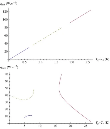
heat flux q_bafS for low solar constants (around 20 W m−2), strong surface heat fluxq_bafP at high solar constants (around 100 W m−2), with an unstable branchq_bafG linking the two.

On the contrary, the surface heat flux obtained through the MEP procedureqmepis much less constrained by the

tem-perature gradient. Figure 12 shows the surface heat flux as a function of the temperature gradientTg−Tafor both cases:

qbafandqmep. It is clear that the two differ completely, not

only because the temperature gradients in the different cli-mates are very different, but also because the shape ofqmep

low. On the warm branch for the MEP state, high values of qmep are obtained for high values of the solar constant.

Hence, decreasing the solar constant brings the surface flux down, until the point where only the snowball state survives, with a similar low value of the surface heat flux.

This discrepancy between the two graphs is likely to be significant: it has been suggested that the suppression of the vertical temperature gradient in the snowball state numbers amongst the reasons that make deglaciation of the snowball Earth so difficult (Pierrehumbert, 2004, 2005; le Hir et al., 2010). Indeed, the temperature inversion isolates the surface from all the forms of energy exchange: the greenhouse ef-fect can only warm the surface when the air aloft is colder, latent heat plays a very limited role in this very dry atmo-sphere, and the sensible heat flux is also restricted by the vertical structure of the atmosphere. Pierrehumbert (2004) points out that a crucial role may be played by the surface fluxes parameterization and the convection parameterization. Here the simplicity of the model does not allow us to discuss the static stability, nor to come up with a clear explanation of the questioning Fig. 12, but it does certainly reinforce the idea that surface heat fluxes parameterization can play criti-cal parts on important paleoclimate problems. In the case of the MEP surface heat flux, our results tend to indicate that it would be possible for the snowball earth to withstand a vertical temperature gradient higher than expected with very little loss in the form of sensible heat, thereby damaging the thermal shield of the surface layer mentioned above.

On a similar note, Lucarini et al. (2010) performed a thor-ough investigation of the thermodynamic properties of the snowball Earth as compared to warm climates in the model of intermediate complexity PLASIM (Fraedrich et al., 2005), using the formalism of non-equilibrium thermodynamics ap-plied to the climate system as described in Lucarini (2009). Computation of the thermodynamics efficiency, irreversibil-ity and material entropy production clearly characterizes dis-tinct thermodynamic regimes for the snowball Earth and ice-free climate. Our remarks about the surface heat flux in snowball conditions add up to their thermodynamic analysis.

4 Conclusions

The analogy developed in this study leads to some enlight-ening conclusions. First, about the ice-albedo feedback in itself, it provides a variational principle different from those previously suggested, with a thermodynamic motivation. On the contrary, all the candidates for variational formulations of the problem examined previously were rather ad hoc tials for the dynamical system. The parallel between poten-tials properly speaking, which fully describe the dynamics of the system, and the entropy production rate, which only characterize equilibrium states, was pushed one step further with the introduction of a method to integrate a trajectory using the MEP principle. In particular we have shown that

0.5 1.0 1.5 2.0 2.5

Tg-T_aHKL

20 40 60 80 100 120

qbafHW.m

-2_L

5 10 15 20 25 Tg

-_TaHKL

10 20 30 40 50 60 70

qmepHW.m

-2_L

Fig. 12. Comparison between the bulk aerodynamic formula sur-face heat flux (top) and the MEP predicted sursur-face heat flux (bot-tom) as a function of the temperature gradientTg−Ta. The red solid

line corresponds to the warm branch of the bifurcation diagram, the blue solid line to the snowball state and the dotted yellow line is the unstable branch. Note the very different scales forTg−Ta.

this method predicts the correct stability for the MEP pre-dicted equilibria. We also investigated the behaviour of the surface heat flux in the snowball state. The results hint that MEP might prove useful in such extreme situations where the usual parameterizations face important difficulties. However, the highly simplified model considered here does not allow us to conclude against or in favour of the MEP parameteriza-tion, as compared to the bulk-aerodynamic formula.

As far as the MEP conjecture is concerned, our work adds up to the relatively short list of efforts up to now (es-sentially Shimokawa and Ozawa, 2001, 2002 and Jupp and Cox, 2010) to sort out how the principle should be under-stood in the presence of multiple entropy production max-ima. Shimokawa and Ozawa (2002) suggested that a dy-namical system, in their case the thermohaline circulation, when multiple steady-states are available, should move to the most dissipative one. Nicolis (2003) and Nicolis and Nicolis (2010) showed strong limitations to this interpretation in full generality. Here, we find that steady-states of a system with

Instead, we suggest that the question of the dynamic stability can be investigated by a relaxation process maximizing the instantaneous entropy production rate.

Acknowledgements. The authors wish to thank two anonymous reviewers for valuable comments.

Edited by: V. Lucarini

The publication of this article is financed by CNRS-INSU.

References

Arnold, V.: Ordinary Differential Equations, Springer, New York, USA, 1984.

Bruers, S.: A discussion on maximum entropy production and in-formation theory, J. Phys. A, 40, 7441–7450, 2007.

Budyko, M.: The effect of solar radiation variations on the climate of the Earth, Tellus, 21, 611–619, 1969.

Cahalan, R. and North, G.: A Stability Theorem for Energy-Balance Climate Models, J. Atmos. Sci., 36, 1178–1188, 1979.

Chylek, P. and Coakley, J.: Analytical analysis of a Budyko-type climate model, J. Atmos. Sci., 32, 675–679, 1975.

Crafoord, C. and K¨all´en, E.: A Note on the Condition for Existence of More than One Steady-State Solution in Budyko-Sellers Type Models, J. Atmos. Sci., 35, 1123–1124, 1978.

Dewar, R.: Information theory explanation of the fluctuation theo-rem, maximum entropy production and self-organized criticality in non-equilibrium stationary states, J. Phys. A, 36, 631–641, 2003.

Dewar, R.: Maximum entropy production and the fluctuation theo-rem, J. Phys. A, 38, 371–381, 2005.

Dufresne, J.-L., Fournier, R., Hourdin, C., and Hourdin, F.: Net exchange reformulation of radiative transfer in the CO₂15 µm band on Mars, J. Atmos. Sci., 62, 3303–3319, 2005.

Faegre, A.: An intransitive model of the Earth-atmosphere-ocean system, J. Appl. Meteorol., 11, 4–6, 1972.

Filyukov, A.: Compatibility property of steady systems, J. Eng. Phys. Thermophys., 14, 814–819, 1968.

Filyukov, A. and Karpov, V.: Description of steady transport pro-cesses by the method of the most probable path of evolution, J. Eng. Phys. Thermophys., 13, 624–630, 1967a.

Filyukov, A. and Karpov, V.: Method of the most probable path of evolution in the theory of stationary irreversible processes, J. Eng. Phys. Thermophys., 13, 798–804, 1967b.

Fraedrich, K.: Structural and stochastic analysis of a zero-dimensional climate system, Q. J. Roy. Meteor. Soc., 104, 461– 474, 1978.

Fraedrich, K., Jansen, H., Kirk, E., Luksch, U., and Lunkeit, F.: The Planet Simulator: Towards a user friendly model, Meteorol. Z., 14, 299–304, 2005.

Frederiksen, J.: Nonlinear albedo-temperature coupling in climate models, J. Atmos. Sci., 33, 2267–2272, 1976.

Gal-Chen, T. and Schneider, S.: Energy balance climate modeling: Comparison of radiative and dynamic feedback mechanisms, Tellus, 28, 108–121, 1976.

Gerard, J., Delcourt, D., and Francois, L.: The maximum entropy production principle in climate models: application to the faint young sun paradox, Q. J. Roy. Meteor. Soc., 116, 1123–1132, 1990.

Ghil, M.: Climate stability for a Sellers-type model, J. Atmos. Sci., 33, 3–20, 1976.

Grassl, H.: The climate at maximum entropy production by merid-ional atmospheric and oceanic heat fluxes, Q. J. Roy. Meteor. Soc., 107, 153–166, 1981.

Grinstein, G. and Linsker, R.: Comments on a derivation and ap-plication of the “maximum entropy production” principle, J. Phys. A, 40, 9717–9720, 2007.

Guckenheimer, J. and Holmes, P.: Nonlinear Oscillations, Dynam-ical Systems, and Bifurcations of Vector Fields, vol. 42 of Ap-plied Mathematical Sciences, Springer, New York, USA, 1983. Held, I. and Suarez, M.: Simple albedo feedback models of the

icecaps, Tellus, 26, 613–629, 1974.

Herbert, C., Paillard, D., Kageyama, M., and Dubrulle, B.: Present and Last Glacial Maximum climates as maximum entropy pro-duction states, Q. J. Roy. Meteor. Soc., submitted, 2010. Jaynes, E.: The minimum entropy production principle, Ann. Rev.

Phys. Chem., 31, 579–601, 1980.

Jupp, T. E. and Cox, P.: MEP and planetary climates: insights from a two-box climate model containing atmospheric dynamics, Phi-los. T. Roy. Soc. B, 365, 1355–1365, 2010.

Kleidon, A. and Lorenz, R.: Non-equilibrium Thermodynamics and the Production of Entropy: Life, Earth, and Beyond, Springer, Berlin, Germany, 2005.

le Hir, G., Donnadieu, Y., Krinner, G., and Ramstein, G.: Toward the snowball earth deglaciation, Clim. Dynam., 35, 285–297, 2010.

Lian, M. and Cess, R.: Energy balance climate models: A reap-praisal of ice-albedo feedback, J. Atmos. Sci., 34, 1058–1062, 1977.

Lorenz, E. N.: Climatic determinism, Meteorol. Monogr., 8, 1–3, 1968.

Lorenz, E. N.: Climatic change as a mathematical problem, J. Appl. Meteorol., 9, 325–329, 1970.

Lorenz, R., Lunine, J., Withers, P., and McKay, C.: Titan, Mars and Earth: Entropy production by latitudinal heat transport, Geophys. Res. Lett., 28, 415–418, 2001.

Lucarini, V.: Thermodynamic efficiency and entropy

produc-tion in the climate system, Phys. Rev. E, 80, 021118, doi:10.1103/PhysRevE.80.021118, 2009.

Lucarini, V., Fraedrich, K., and Lunkeit, F.: Thermodynamic analy-sis of snowball Earth hystereanaly-sis experiment: Efficiency, entropy production and irreversibility, Q. J. Roy. Meteor. Soc., 136, 2–11, 2010.

Martyushev, L. and Seleznev, V.: Maximum entropy production principle in physics, chemistry and biology, Physics Reports, 426, 1–45, 2006.

2010.

Nicolis, C.: Comment on the connection between stability and en-tropy production, Q. J. Roy. Meteor. Soc., 129, 3501–3504, 2003. Nicolis, C. and Nicolis, G.: Stability, complexity and the maximum dissipation conjecture, Q. J. Roy. Meteor. Soc., 136, 1161–1169, 2010.

North, G.: Analytical solution to a simple climate model with dif-fusive heat transport, J. Atmos. Sci., 32, 1301–1307, 1975a. North, G.: Theory of energy-balance climate models, J. Atmos.

Sci., 32, 2033–2043, 1975b.

North, G., Howard, L., Pollard, D., and Wielicki, B.: Variational formulation of Budyko-Sellers climate models, J. Atmos. Sci., 36, 255–259, 1979.

North, G., Cahalan, R., and Coakley, J.: Energy Balance Climate Models, Rev. Geophys. Space Phys., 19, 91–121, 1981. Oerlemans, J. and van den Dool, H.: Energy balance climate

mod-els: Stability experiments with a refined albedo and updated coefficients for infrared emission, J. Atmos. Sci., 35, 371–381, 1978.

Ozawa, H. and Ohmura, A.: Thermodynamics of a global-mean state of the atmosphere – a state of maximum entropy increase, J. Climate, 10, 441–445, 1997.

Ozawa, H., Ohmura, A., Lorenz, R., and Pujol, T.: The second law of thermodynamics and the global climate system: A review of the maximum entropy production principle, Rev. Geophys., 41, 1018, 2003.

Paltridge, G.: Global dynamics and climate-a system of minimum entropy exchange, Q. J. Roy. Meteor. Soc., 101, 475–484, 1975. Paltridge, G.: The steady-state format of global climate, Q. J. Roy.

Meteor. Soc., 104, 927–945, 1978.

Paltridge, G.: Climate and thermodynamic systems of maximum dissipation, Nature, 279, 630–631, 1979.

Peixoto, J. P. and Oort, A. H.: Physics of Climate, Springer, New York, USA, 1992.

Pierrehumbert, R.: High levels of atmospheric carbon dioxide nec-essary for the termination of global glaciation, Nature, 429, 646– 649, 2004.

Pierrehumbert, R.: Climate dynamics of a hard snowball Earth, J. Geophys. Res., 110, D01111, doi:10.1029/2004JD005162, 2005. Pujol, T. and Fort, J.: States of maximum entropy production in a one-dimensional vertical model with convective adjustment, Tel-lus, 54, 363–369, 2002.

Robert, R. and Sommeria, J.: Relaxation towards a statistical equi-librium state in two-dimensional perfect fluid dynamics, Phys. Rev. Lett., 69, 2776–2779, 1992.

Schneider, S. and Gal-Chen, T.: Numerical experiments in climate stability, J. Geophys. Res., 78, 6182–6194, 1973.

Sellers, W.: A global climatic model based on the energy balance of the earth-atmosphere system, J. Appl. Meteorol., 8, 392–400, 1969.

Shimokawa, S. and Ozawa, H.: On the thermodynamics of the oceanic general circulation: entropy increase rate of an open dissipative system and its surroundings, Tellus A, 53, 266–277, 2001.

Shimokawa, S. and Ozawa, H.: On the thermodynamics of the oceanic general circulation: Irreversible transition to a state with higher rate of entropy production, Q. J. Roy. Meteor. Soc., 128, 2115–2128, 2002.