IFC 4
(4
thInternational Finance Conference)
15-16-17 March 2007 - Tunisia
Topic: Modelling and Forecasting
A new approach to modelling and forecasting monthly overnights in the Northern
Region of Portugal
Paula Odete Fernandesa,* ([email protected]), João Paulo Teixeirab ([email protected]) a
Department of Economics and Management, Polytechnic Institute of Bragança, Portugal b
Department of Electrical Engineering, Polytechnic Institute of Bragança, Portugal
*
Corresponding Author: +351 273 303 103; Fax: +351 273 313 051 Escola Superior de Tecnologia e de Gestão (ESTiG)
Instituto Politécnico de Bragança (IPB) Campus de Sta. Apolónia, Apartado 134
Abstract
The need to analyze the main factors determining the evolution of demand within the tourism sector, which is the driving force of the whole tourism activity, and the importance that forecasting has in this domain, may be justified by the fact that the tourism sector plays a significant role in the economy of Portugal and its regions because of the large number of people employed directly and indirectly, and also because of its ability to bring in currency that reflects in different sector of economic activity.
Although tourism is less developed in the North of Portugal than in other regions of the country, it is essential to comprehend this phenomenon in order to empower local economic agents to carry out strategic measures to maximize profits from newly emerging situations.
The objective of the present research is to quantify national and international tourism flows by developing (mathematical) models and applying them to sensitivity studies in order to predict demand.
This work provides a deeper understanding of the tourism sector in Northern Portugal and contributes to already existing econometric studies by using the Artificial Neural Networks methodology.
This work's focus is on the treatment, analysis, and modelling of time series representing “Monthly Guest Nights in Hotels” in Northern Portugal recorded between January 1987 and December 2003. This was achieved through a study of the reference time series whose past values were known and whose objective was to obtain a model that better predicts the behaviour of the time series under study.
The model used 6 neurons in the hidden layer with the logistic activation function and was trained using the Resilient Backpropagation algorithm (a variation of backpropagation algorithm). Each time series forecast depended on 12 preceding values. The obtained model yielded acceptable goodness of fit and statistical properties and is therefore adequate for the modelling and prediction of the reference time series.
1.INTRODUCTION
Several empirical studies in the tourism scientific area have been performed and published in the last decades. These studies agree in the consideration that the forecast process in the tourism sector must be done with particular care.
Nowadays, there is a great variety of models or methods for forecasting (from the most simple to the most complex ones) that have been developed for a variety of situations and present different characteristics and methodologies.
In this context, and related to tourism demand in Northern Portugal, a study has been carried out with the reference temporal sequence -“Monthly Guest Nights in Hotels”- using known previous values aiming to build a model that better fits the behaviour of the sequence. For this purpose the model used is supported in Artificial Neural Networks (ANN). The methodology of the ANN was inspired in the biologic theories of human brain function. The human brain is composed of several non-linear processors densely interconnected operating in parallel, these being the principal advantages compared with other forecast techniques.
This paper is organized in the following structure: first, there is an overview section that examines the theoretical foundation of neural networks. This section, in particular, analyzes the use of ANN models as a forecasting tool for business applications. Based on the theoretical analysis, a neural network is developed for forecasting tourism demand in Northern Portugal. Real data from official publications in Portugal is used for the neural network development. The model development process, the empirical and analysis results of forecasting are described in the next section. The quality of forecasting results is measured in mean absolute percentage error. Some concluding remarks are given in the final section.
2. Neural Network Models
Artificial Neuronal Networks has been developed as generalizations of mathematical models of human cognition or neural biology, based on the assumptions (Rumelhard & McClelland, 1986a, 1986b) that:
a. Information processing occurs at several simple elements that are called neurons;
b. Signals are passed between neurons over connection links;
c. Each connection link has an associated weight, which, in a typical neural net, multiplies the signal transmitted;
d. Each neuron applies an activation function (usually nonlinear) to its net input (sum of weighted input signals) to determine its output signal.
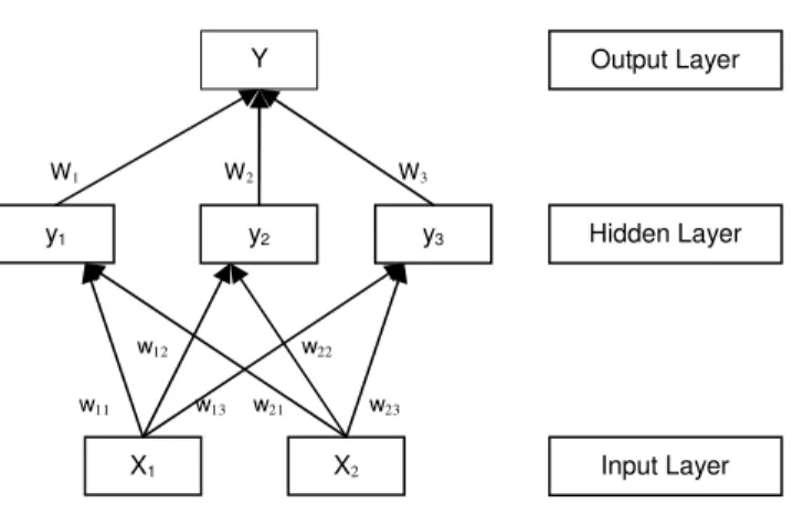
Through replicate learning process and associative memory, the ANN model can accurately classify information as pre-specified pattern. A typical ANN consists of a number of simple processing elements called neurons, nodes or units. Each neuron is connected to other neurons by means of directed communication links. Each connection has an associated weight. The weights are the parameters of the model being used by the net to solve a problem. ANNs are usually modelled into one input layer, one or several hidden layers, and one output layer (Tsaur et al., 2002). Fig. 1 demonstrates a simplified neural network with three layers.
Fig. 1: A neural network model.
In Fig. 1, each node in the hidden layer computes yj(j=1, 2, 3)according to expression [1] (Haykin, 1999):
2
1
j i ji
i
f x w
=
= [1]
In addition, a sigmoid function(yj), in the following form, is used to transform the output that is limited into
an acceptable range. The purpose of a sigmoid function is to prevent the output being too large, as the value of yj(for j=1, 2, 3) must fall between 0 and 1:
w13 w22
w23 w21
w12
W2 W3
W1
w11
Y
y1 y2 y3
X1 X2
Output Layer
Hidden Layer
1
1 j
j f
y
e− =
+ [2]
Finally, Yin the node of the output layer in Fig. 1 is obtained by the following summation function:
3
1 j j j
Y
y w
=
=
[3]
Nodes in the input layer represent independent parameters of the system. The hidden layer is used to add an internal representation handling non-linear data. The output of the neural network is the solution for the problem. A feedforward neural network learns from a supervised training data to discover patterns connecting input and output variables. Feedforward recall is a one-directional information processing neural network in which the signal flows from the input units to the output units in a forward direction (Kuan & White, 1994; Nam & Schaefer, 1995; Yao et al., 2000).
Backpropagation is the most popular neural network training algorithm that has been used to perform learning on feedforward neural networks. It is a method for assigning responsibility for mismatches to each of the processing units in the network, which is achieved by propagating the gradient of the activation function back through the network to each hidden layer, down to the first hidden layer. The weights are then modified so as to minimize the mean squared error between the network’s prediction and the actual target (Thawornwong & Enke; 2004). The Backpropagation neural network consists of an input layer, an output layer and one or more intervening layers also referred to as hidden layers. The hidden layers can capture the nonlinear relationship between variables. Each layer consists of multiple neurons that are connected to neurons in adjacent layers. Since these networks contain many interacting nonlinear neurons in multiple layers, the networks can capture relatively complex phenomena (Hill, O’Connor & Remus, 1996; Chiang, Urban & Baldridge; 1996; Basheer & Hajmeer; 2000). Many variant were developed of Backpropagation training algorithm. In our case we adopted the Resilient Backpropagation
[RP] (Reidmiller & Braun, 1993), because it can combine fast convergence, stability and generally good results.
Usually, the learning process involves the following stages (Zhang, 2003; Fernandes, 2005): 1. Assign random numbers to the weights;
2. For every element in the training set, calculate output using the summation functions embedded in the nodes;
3. Compare computed output with observed values;
4. Adjust the weights and repeat steps (2) and (3) if the result from step (3) isn’t less than a threshold value; alternatively, this cycle can be stopped early by reaching a predefined number of iterations, or the performance in a validation set does not improve.
3. A neural network model for forecasting tourism demand in Northern Portugal 3.1 Methodology
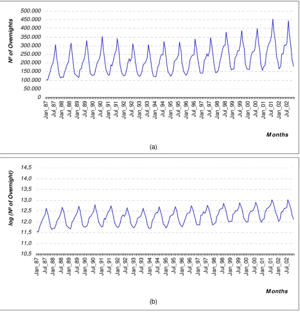
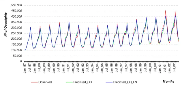
For the selection of data we used the secondary source published in the Portuguese National Statistical Institute. Table A.1, in Appendix, containing relevant data for forecasting MonthlyGuest Nights in Hotels in the North of Portugal recorded between January 1987 and December 2003. The Northern region of Portugal is delimited in Fig 2. During this study we call this time series Original Data (OD) (Fig. 3a). This time series suggests a power transformation, we take logarithms of the data to stabilize the seasonality and variance, and we have another time series - the Transformed Original Data (OD_Ln) (Fig. 3b).
R. A. Açores
R. A. Madeira
Algarve Alentejo Lisboa
Centro Norte
Km 0 50
Leyenda
Límite de NUT II 0 50 km
Fig. 2: Regions of Portugal.
0 50.000 100.000 150.000 200.000 250.000 300.000 350.000 400.000 450.000 500.000 J a n _ 8 7 J u l_ 8 7 J a n _ 8 8 J u l_ 8 8 J a n _ 8 9 J u l_ 8 9 J a n _ 9 0 J u l_ 9 0 J a n _ 9 1 J u l_ 9 1 J a n _ 9 2 J u l_ 9 2 J a n _ 9 3 J u l_ 9 3 J a n _ 9 4 J u l_ 9 4 J a n _ 9 5 J u l_ 9 5 J a n _ 9 6 J u l_ 9 6 J a n _ 9 7 J u l_ 9 7 J a n _ 9 8 J u l_ 9 8 J a n _ 9 9 J u l_ 9 9 J a n _ 0 0 J u l_ 0 0 J a n _ 0 1 J u l_ 0 1 J a n _ 0 2 J u l_ 0 2 M onths N º o f O v e rn ig h ts (a) 10,5 11,0 11,5 12,0 12,5 13,0 13,5 14,0 14,5 J a n _ 8 7 J u l_ 8 7 J a n _ 8 8 J u l_ 8 8 J a n _ 8 9 J u l_ 8 9 J a n _ 9 0 J u l_ 9 0 J a n _ 9 1 J u l_ 9 1 J a n _ 9 2 J u l_ 9 2 J a n _ 9 3 J u l_ 9 3 J a n _ 9 4 J u l_ 9 4 J a n _ 9 5 J u l_ 9 5 J a n _ 9 6 J u l_ 9 6 J a n _ 9 7 J u l_ 9 7 J a n _ 9 8 J u l_ 9 8 J a n _ 9 9 J u l_ 9 9 J a n _ 0 0 J u l_ 0 0 J a n _ 0 1 J u l_ 0 1 J a n _ 0 2 J u l_ 0 2 M onths lo g ( N º o f O v e rn ig h t) (b)
Fig. 3: Overnights in the North of Portugal from 1987:01 to 2002:12: (a) Original Data; (b) Natural Logarithms.
The ANN model used in this study is the standard three-layer feedforward network. Since the one-step-ahead forecasting is considered, only one output node is employed. The activation function for hidden nodes is the logistic function [Logsig]: ( ) 1( )
1 e x
f x
−
=
+ ; and for the output node the identity function
(pure linear function) [Lin]: f x( )=x. Bias terms are used in both hidden and output layer’s nodes. The fast
architecture consists of 12 input nodes in the entrance layer, 6 hidden nodes in the second layer and one node in the output layer - (1-12;6;1). The input of the model consists of the 12 previous numbers - corresponding to the last 12 months overnights. The output is the predicted overnights for the next month. To make monthly predictions we have combined the following suppositions: consider as delayed inputs the most previous observations of the month we are predicting; due to the seasonal behaviour of the series we use a period of one year - twelve months.
In the training process of an ANN different end points are achieved, although with similar performance, for different initial values. Therefore, several training sessions for each identified situation have been performed with different initial weights. From this number of training sessions we retain the ANN (concerning its weights) that obtain better forecast results in each situation under the validation set. In this particular situation we performed 500 training sessions.
In order to compare the performance, the root mean squared error (RMSE1) between the observed and predicted values are used as the agreement index. The other agreement index used in this paper is the coefficient of correlation2 between the observed and predicated values. We adopted the first index to select the best model/ANN.
Also in the training process, for each session we need to establish the number of iterations and the goal. In the present study we defined our goal as an error (RMSE between target and predicted values) of the order of 1x10⁻⁴. Anyhow, the training never stopped due to the achievement of this goal nor even by the predefined maximum number of iterations, but because of an early stop training condition.
The data set was divided in a sub-set for training, a sub-set for validation and a sub-set for test. The data set between January 1988 until December 2001 (in a total of 168 months) was used for training. It must be notice that the data between January and December 1987 was used as the input data for predicting January 1988 till December. The data between January and December 2002 was used for the validation set. This set is used for early stop training if the RMSE does not decrease in a number (5 in this case) of training iterations. This early stop training condition avoids the ANN to over fit the training data without improvements in a data not used in the training phase. Finally the data between January and December 2003 was used as data never seen in the training and selection process and used just to present the results of the model with never seen data.
1 ( )
2
1 ;
n
t t
t
A P RMSE
n
=
− =
2
(
)(
)
(
) (
)
1 ,
2 2
; .
n
t t
t
A P n
A A P P r
A A P P
=
− −
=
For an ANN model the prediction equation for computing a forecast ofYtusing selected past observations
can be written as (Fernandes, 2005):
2,1 1,
1 1
n m
t j ij t i j
j i
Y
b
w f
W y
−b
= =
=
+
+
[4]where,
m
, is the number of input nodes;n
, is the number of hidden nodes;f
, is a sigmoid transfer function such as the logistic;{
w j
j,
=
0,1,
,
n
}
, is a vector of weights from the hidden to output nodes;{
W i
ij,
=
0,1,
, ;
m j
=
1, 2,
,
n
}
, are weights from the input to hidden nodes;2,1
b
andb
1,j, are the bias associated with the nodes in output and hidden layers, respectively.The equation shows a linear transfer function used in the output node.
In both models, for each time series, the resilient backpropagation algorithm was used for train the ANN. The sigmoid logistic activation function was used in the hidden layer nodes. The total number of parameter of the used ANN is 85. These alternatives are justified in Fernandes (2005) because of their improved results.
3.2. Empirical Analysis of the Results
In this section we will examine the results of each ANN under the test set. For this purpose we will compare the predicted data of each ANN with the target values for the year 2003 (the test set). We should emphasize that the target data is the original data of the time series and was never seen by the model in the training phase nor even in the selection process of the model. The selection process of the better ANN is governed by the minimum RMSE in the training set.
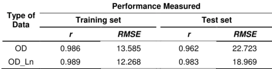
Table 1 presents for each ANN time series the performance measured by both the r (correlation coefficient) and the RMSE in the training set and test set.
Table 1: Results of ANNs models.
Performance Measured
Training set Test set
Type of Data
r RMSE r RMSE
OD 0.986 13.585 0.962 22.723
Between both time series (original - OD, and transformed - OD_Ln) the transformed one is where the lower RMSE was achieved with correlation coefficient of 0.989 in the training set. We can never say that this is the better model, but comparing the results of the prediction between both implemented models and considering that these models resulted from a selection of several different architectures we can say that the final results are stable and has and interesting performance. Therefore, this model is selected based only in the training set.
We should look now at the performance in the test set. Regarding the performance in the test set presented in Table 1 the previous selected model (using OD_Ln) is confirmed now with lower RMSE and higher r. Both measures RMSE and r are better in the model using the transformed time series. Although the RMSE becomes deteriorated now, the correlation coefficient stills at a relatively high level.
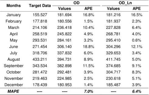
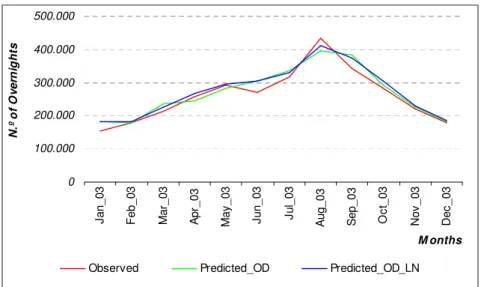
The predicted values for the year of 2003 (data used as the test set) with both models and its APE and MAPE are presented in Table 2. APE is the absolute percentage error given by the expression [5]. MAPE is the Mean absolute percentage error given by the expression [6].
ˆ
100.
t tt
Y
Y
Y
=
−
×
APE [5]
1 ˆ 1
100. N
t t
t t
Y Y N = Y
−
= ×
MAPE
[6]
Table 2: Prediction of the forecasting ANN models, APE and MAPE in the period 01/2003 to 12/2003.
OD OD_Ln
Months Target Data
Values APE Values APE
January 155.527 181.694 16.8% 181.216 16.5%
February 177.818 180.556 1.5% 181.937 2.3%
March 214.106 236.418 10.4% 227.828 6.4%
April 258.519 245.822 4.9% 268.781 4.0%
May 293.531 284.161 3.2% 295.410 0.6%
June 271.454 306.140 18.8% 304.296 12.1%
July 318.706 337.832 6.0% 329.653 3.4%
August 433.211 394.731 8.9% 411.745 5.0%
September 343.534 382.898 11.5% 374.685 9.1%
October 281.472 292.481 3.9% 304.717 8.3%
November 219.463 224.985 2.5% 230.618 5.1%
December 178.439 180.953 1.4% 185.487 3.9%
MAPE ---- ---- 7.0% ---- 6.4%
According to the Criteria of MAPE for Model Evaluation in Lewis (1982), presented in Table 3, the predicted data with the selected model has an highly accurate forecast.
Table 3: Criteria of MAPE for Model Evaluation.
MAPE (%) Assessment
<10 Highly Accurate Forecasting
10-20 Good Forecasting
20-50 Reasonable Forecasting
>50 Inaccurate Forecasting
Source: Lewis (1982).
Figure 4 displays the original and predicted time series for the 12 months of 2003 with both models. Both models follow the behaviour of the target data. Figure 5 displays the same data for the entire time series. As expected the predicted date fits better the target data in the training set than in the never previously seen test data. In Figure 5 we can observe an additional difficulty for the model imposed by the fact that years 2001 to 2003 have had and increasing number of overnights, and this increasing phenomena was present in the training set only in 2001. This phenomenon was due to the fact that the city of Guimarães and the Douro Region were considered World Cultural Heritage, and the city of Porto was the European Capital of Culture in 2001.
0 100.000 200.000 300.000 400.000 500.000
J
a
n
_
0
3
F
e
b
_
0
3
M
a
r_
0
3
A
p
r_
0
3
M
a
y
_
0
3
J
u
n
_
0
3
J
u
l_
0
3
A
u
g
_
0
3
S
e
p
_
0
3
O
c
t_
0
3
N
o
v
_
0
3
D
e
c
_
0
3
M onths
N
.º
o
f
O
v
e
rn
ig
h
ts
Observed Predicted_OD Predicted_OD_LN
0 50.000 100.000 150.000 200.000 250.000 300.000 350.000 400.000 450.000 500.000 J a n _ 8 7 J u l_ 8 7 J a n _ 8 8 J u l_ 8 8 J a n _ 8 9 J u l_ 8 9 J a n _ 9 0 J u l_ 9 0 J a n _ 9 1 J u l_ 9 1 J a n _ 9 2 J u l_ 9 2 J a n _ 9 3 J u l_ 9 3 J a n _ 9 4 J u l_ 9 4 J a n _ 9 5 J u l_ 9 5 J a n _ 9 6 J u l_ 9 6 J a n _ 9 7 J u l_ 9 7 J a n _ 9 8 J u l_ 9 8 J a n _ 9 9 J u l_ 9 9 J a n _ 0 0 J u l_ 0 0 J a n _ 0 1 J u l_ 0 1 J a n _ 0 2 J u l_ 0 2 M onths N º o f O v e rn ig h ts
Observed Predicted_OD Predicted_OD_LN
Fig. 5: Comparison between Original Data and Predicted Values, in the training data and validation data sets.
4.CONCLUSIONS
This paper describes the process of modelling tourism demand for the north of Portugal, using an artificial neural network model. Data used in the time series was obtained from official publications - Portuguese National Statistics Institute. The time series was considered in two different ways; one was the original data and another was the logarithmic transformed data. Both series were separate into a training data set to train the neural network, in a validation set, to stop the training process earlier and a test data set to examine the level of forecasting accuracy.
The model has 6 neurons in the hidden layer with the logistic activation function and was trained using the
Resilient Backpropagation algorithm(a variation of backpropagation algorithm). The ANN model has the 12 preceding values as the input. The analysis of the output forecast data of the selected ANN model showed a relatively close result compared to the target data. In other words, the model produced, according to Lewis (1982) a highly accurate forecast. Therefore it can be considered adequate for the purpose of prediction in the reference time series.
The model applied to the logarithmic transformed data achieved better results evaluated by the RMSE, the correlation coefficient and MAPE.
Considering the results, the artificial neural network based models represent an effective alternative to classical models in tourism forecasting. This methodology becomes interesting to forecast because it allows the use of a non linear model for seasonal time series.
R
EFERENCESBasheer, I.A. and Hajmeer, M.; (2000); “Artificial Neural Networks: fundamentals, computing, design and application”; Journal of Microbiological Methods; N.º 43, pp.3/31.
Chiang, W.C.; Urban, T.L. and Baldridge, G.W.; (1996); “A neural network approach to mutual fund net asset value forecasting”; Omega, The International Journal of Management Science; Vol. 24, N.º 2, pp. 205/215.
Fernandes, Paula Odete; (2005); “Modelación, Predicción y Análisis del Comportamiento de la Demanda Turística en la Región Norte de Portugal”; Dissertação de Doutoramento em Economia Aplicada e Análise Regional; Universidade de Valladolid.
Haykin, Simon; 1999; “Neural Networks. A comprehensive foundation”;New Jersey, Prentice Hall.
Hill, Tim; O’Connor, Marcus and Remus, William; (1996); “Neural network models for time series forecasts”; Management Science; Vol. 42, N.º 7, pp.1082/1092.
Kuan, Chung-Ming and White, Halbert; (1994); “Artificial Neural Network: An econometric perspective”;
Econometric Reviews;N.º 13, pp.1/91.
Lewis, C.D.; (1982); “Industrial and Business Forecasting Method”; Butterworth Scientific; London.
Nam, Kyungdoo and Schaefer, Thomas; (1995); “Forecasting International Airline Passenger Traffic Using Neural Networks”; Logistics and Transportation Review; Vol. 31, N.º 3, pp.239/251.
Pattie, Douglas C. and Snyder, John; (1996); “Using a neural network to forecast visitor behaviour”;
Annals of Tourism Research; Vol. 23, N.º 1, pp.151/164.
Reidmiller, M and Braun, H.; (1993); “A direct adaptive method for faster backpropagation learning: The RPRO algorithm. Proceedings of the IEEE International Conference on Neural Networks.
Thawornwong, Suraphan and Enke, David; (2004); “The adaptive selection of financial and economic variables for use with artificial neural networks”; Neurocomputing; N.º 56, pp.205/232.
Tsaur, Sheng-Hshiung; Chiu, Yi-Chang and Huang, Chung-Huei; (2002); “Determinants of guest loyalty to international tourist hotels-a neural network approach”; Tourism Management; N.º 23, pp.397/405.
Yao, Jingtao; Li, Yili and Tan, Chem Lim; (2000); “Option price forecasting using neural networks”;
Omega, The International Journal of Management Science; N.º 28, pp.455/466.
Zhang, G. Peter; (2003); “Time series forecasting using a hybrid ARIMA and neural network model”;
APPENDIX A
Table A.1: Overnights in the North of Portugal from 01/1987 to 12/2003 Original Data. YEAR
MONTH
1987 1988 1989 1990 1991 1992 1993 1994 1995 1996 1997 1998 1999 2000 2001 2002 2003
January 102.447 118.011 122.217 126.671 126.826 124.194 121.469 118.606 122.480 126.910 140.430 148.218 163.696 162.389 176.690 165.653 155.527
February 102.123 117.547 116.837 129.802 131.653 127.474 129.284 122.988 130.393 139.403 141.183 157.415 165.988 162.637 186.586 181.005 177.818 March 125.401 142.687 160.658 158.701 188.999 157.536 154.734 175.261 156.645 172.393 219.465 209.929 228.149 226.010 245.261 249.214 214.106
April 150.042 167.118 169.326 197.757 182.290 196.087 189.142 185.525 209.263 213.973 224.382 232.767 242.744 262.865 291.395 253.274 258.519
May 180.430 189.823 199.158 207.876 219.187 223.918 198.402 232.075 218.666 239.142 253.833 280.326 269.854 264.497 306.743 302.028 293.531 June 197.113 207.729 218.595 227.159 251.295 207.907 207.216 248.237 222.720 245.264 238.334 296.612 270.126 273.881 325.568 301.465 271.454
July 229.293 254.523 252.634 257.633 273.927 231.801 231.453 246.274 247.589 248.398 266.993 303.866 306.031 324.962 351.955 314.560 318.706 August 304.847 315.113 329.014 351.500 341.490 312.026 304.576 322.366 320.750 336.086 345.672 377.645 385.868 397.405 452.581 444.991 433.211
September 238.542 258.287 278.074 284.867 283.378 259.023 249.583 266.094 269.433 280.769 288.409 309.700 321.248 331.155 383.793 361.181 343.534
October 173.503 174.359 189.664 216.286 197.241 205.400 202.792 206.256 196.466 225.734 232.052 263.522 280.597 263.217 319.417 287.383 281.472 November 130.187 137.933 138.683 162.062 152.554 149.289 141.976 144.803 152.340 175.438 166.835 180.796 193.062 186.445 238.925 221.910 219.463
December 114.229 128.774 127.730 139.683 132.802 130.963 120.748 139.706 140.643 143.163 141.349 161.273 166.990 157.210 202.351 179.766 178.439
TOTAL 2.048.157 2.211.904 2.302.590 2.459.997 2.481.642 2.325.618 2.251.375 2.408.191 2.387.388 2.546.6732.658.937 2.922.0692.994.353 3.012.6733.481.265 3.262.430 3.145.780
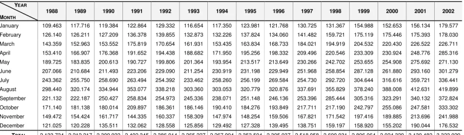
Table A.2: Experimental results of forecasting tourism demand in the north of Portugal in the period 01/1988 to 12/2002. YEAR
MONTH
1988 1989 1990 1991 1992 1993 1994 1995 1996 1997 1998 1999 2000 2001 2002
January 109.463 117.716 119.384 122.864 129.332 116.654 117.350 123.981 121.768 130.725 131.367 154.988 152.653 156.134 179.577
February 126.140 126.211 127.209 136.378 139.855 132.873 132.226 137.824 134.060 141.482 159.721 175.119 175.446 175.393 178.030
March 143.359 152.963 153.552 175.819 170.654 161.931 153.435 163.834 168.733 184.021 194.919 204.532 220.430 226.522 226.711 April 153.410 166.907 176.368 191.652 194.438 188.682 171.950 195.256 198.332 209.496 220.546 233.309 230.924 248.776 285.316
May 189.725 183.835 200.613 190.727 199.806 201.364 193.954 213.517 213.649 230.266 242.702 253.655 254.908 275.692 271.130 June 207.066 210.684 211.493 223.206 229.090 211.254 230.919 231.198 229.949 251.968 258.854 287.128 261.880 293.160 301.279
July 243.362 255.750 258.690 263.494 254.392 233.462 258.260 256.199 269.584 254.730 292.720 304.644 316.616 359.721 336.441 August 298.440 320.174 334.944 353.077 338.218 303.360 303.053 320.779 320.876 337.691 355.829 378.240 388.008 412.631 419.899
September 221.132 222.187 250.427 258.834 254.973 245.336 238.071 251.148 246.136 253.396 285.444 305.316 323.291 340.132 372.824