Proximity Heating Effects in Power Cables

Proximity Heating Effects in Power Cables

Jonathan Blackledge, Eugene Coyle and Kevin O’Connell

Abstract—This paper relates to the study of power system harmonics in the built environment and in particular, cable heating caused by proximity effects due to harmonic distortion. Although in recent years, some movement has taken place in the standards to offer harmonic de-rating factors, heating in cables due to skin and proximity effects has not been quantified effectively. Thus, in this paper we present a model for proximity heating and consider numerical simulations to assess this effect in both two- and three-dimensions for different harmonics. Example results are presented to illustrate the model developed which is based on a general solution for the Magnetic Vector Potential in the Fresnel zone. The model provides the basis for using voxel modelling systems to investigate proximity effects for a range of configurations and complex topologies with applications to the design of power cables, cable trays and ducts, inter-connections, busbar junctions and transformers, for example.

Index Terms—AC power cables, electromagnetic induction, proximity heating effects, harmonic distortion, Fresnel zone simulation.

I. INTRODUCTION

U

NDER ideal circumstances electrical power supply voltage and current waveforms should be sinusoidal. However, this is very seldom the case in the built environ-ment due to the proliferation of non-linear loads. Examples of non-linear loads are those containing switched mode power supplies, reactors and electronic rectifiers/inverters. Common devices such as personal computers, fluorescent lighting, electric motors, variable speed drives, transformers and reactors and virtually all other electrical and electronic equipment are examples of non-linear loads which are the norm in the built environment rather than the exception. Such loads produce complex current and voltage waves and simple spectral analysis of these waves shows that they can be represented by a wave at the fundamental power frequency plus other wave forms at integer and non-integer multiples of this frequency. These harmonics produce an overall effect called ‘Harmonic Distortion’ which can give rise to overheating in plant equipment and the power cables supplying them leading to reduced efficiency, operational life time and on occasions, failure.

Alternating Current (AC) power systems are subject to dis-tortion by harmonic and inter-harmonic components which are present in the supply voltage and load currents. Over the last few decades, harmonic distortion in power supplies has increased significantly due to the increasing use of electronic components in industry and elsewhere. Buildings such as modern office blocks, commercial premises, factories, hos-pitals etc. contain equipment that generates harmonic loads

Manuscript completed in April, 2013.

Jonathan Blackledge ([email protected]) is the Science Foun-dation Ireland Stokes Professor at Dublin Institute of Technology (DIT). Eugene Coyle ([email protected]) is Head of Research Innovation and Partnership and Dublin Institute of Technology. Kevin O’Connell ([email protected]) was formally Head of the Department of Electrical Services Engineering at Dublin Institute of Technology.

as described above. Each item of equipment produces a unique harmonic signature and therefore a harmonic distor-tion which can be predicted if the equipment in use can be determined in advance. Identifying the harmonic signatures of different types of equipment commonly used and the prediction of thermal loading effects on distribution cables caused by the skin and proximity effects of harmonic currents has therefore become increasingly important.

Harmonics can have detrimental effects on the supply system causing a reduction in power quality and consumers equipment connected to the supply can:

1) be adversely affected by existing harmonics, and; 2) generate harmonic currents that create or add to

exist-ing distortion.

It is estimated that losses caused by poor power quality cost EU industry and commerce about 10 billion Euros per annum [1]. Harmonic Standards have therefore been created to set acceptable levels of:

• voltage distortions present in supply systems;

• load current distortion in installations connected to the supply system;

• Electromagnetic Compatibility (EMC) for equipment connected to the supply;

• electromagnetic emissions generated by equipment con-nected to the supply.

Harmonic Standards have also been harmonised interna-tionally to promote international trade so that equipment manufactured in one country will comply with emission and immunity limits in force in other countries.

A. Harmonic Standards

The International Electrotechnical Commission (IEC) based in Geneva is the body responsible for electric power quality standards under which harmonics fall. These stan-dards are referred to as the Electromagnetic Compatibility (EMC) Standards and for the most part are covered by the IEC 61000 series [2] applicable in the EU. Other widely accepted international standards are the IEEE Std 519-1992 [3], ER G5/4-1 [2] and EN 50160 [1]. International standards are used as a basis for global coordination but individual countries may make their own adjustments to the international standards to reflect the special characteristics of their distribution systems. For example, in the case of the UK and Ireland, there are many distributed generation centres located close to many load centres. This presents a different system characteristic to the distribution system in New Zealand, for example, which is characterised by a small number of generating centres connected by long transmission lines to individual load centres [4].

The converse is true of high impedance systems which are referred to as ‘soft systems’. The standards quote higher acceptable levels of harmonic currents for ‘hard’ systems. In setting standards, one must be cognisant of a situation where a large industrial consumer is connected to the supply network together with a number of smaller consumers at a point of common coupling. Were the limits of harmonic current emissions set in absolute terms rather than as a proportion of the consumers load, this may discriminate against the large consumer. If the reverse were the case, this may discriminate against the smaller consumer whose harmonic emissions may be high as a proportion of their load but insignificant in terms of their effect on the system as a whole. It is for this reason and other parallel situations that harmonic standards are issued as guidelines to be applied taking local conditions into account. They are intended to be flexible and applied in a sensible manner. The EMC require-ments in the European Union for electrical and electronic products are covered by the EMC Directive 89/336/EEC [5] which came into effect on 1st January 1996. This directive has been amended a number of times, the most recent being 93/68/EEC in 2004. The Directive seeks to remove technical barriers to trade by requiring equipment to operate satisfactorily in its specified electromagnetic environment. Limiting these emissions serves public electricity distribution systems which must be protected from disturbances emitted by equipment.

National governments are required to enact laws in order to have harmonised standards at European level. These standards must replace the corresponding national provisions. The Electromagnetic Compatibility Regulations 1992 (SI 1992/2372) implemented the Electromagnetic Compatibility Directive 89/336/EEC into UK Law. In Ireland, Statutory Instruments S.I. No. 22/1998 European Communities (Elec-tromagnetic Compatibility) Regulations, 1998, gave legal effect to Directive 89/336/EEC and S.I. No. 109 of 2007. The European Communities (Electromagnetic Compatibility) Regulations, 2007 gave legal effect to Directive 2004/108/EC of the European Parliament and of the Council of 15 Decem-ber 2004 on the approximation of the laws of the MemDecem-ber States relating to electromagnetic compatibility and repealing Directive 89/336/EEC. Engineering Recommendation G5/4-1 [4] came into force in October 2005 to ensure compliance for all system voltages from 400 V to 400 kV in the UK. In Ireland, the CENELEC Standard EN 50160 Voltage Characteristics of Electricity Supplied by Public Networks is used as a basis for compliance.

Harmonic distortion limits are not governed by statute. The legally enforcing document is therefore the connection agree-ment between the network operator and the customer. This agreement lays down connection conditions which require compliance with ER G5/4-1, IEE Std 519-1992 or IEC 50160 and include any derogation and/or harmonic mitigation mea-sures which may be agreed between the network operator and the customer. However, one of the most important issues in the industry is that rating factors tend to ignore the heating effects generated by the higher harmonics. This issue is the theme of the research reported in this paper.

B. About this Paper

Being able to accurately model harmonic proximity effects in the design of cables, junctions, transformers and electrical appliances in general is particularly important in the design of electrical installations. It is important to be able to simulate potential ‘hotspots’ in the built environment and check that heating effects conform to international standards especially with regard to the effect of higher order harmonics. This is because the heat generated is proportional to the square frequency of the harmonic. The two-dimensional cross sectional geometry of modern cables (e.g. see Figure 1) necessitates the accurate simulation of harmonic proximity effects in two-dimensions. The three-dimensional topological complexity of high current busbar interconnections (e.g. see Figure 2) contained inside switchgear, panel boards or busbars and carrying tens of thousands of amperes used in electrochemical production, for example, necessitate the use of full three-dimensional simulation. Flat and hollow topolo-gies are used that allow heat to dissipate more efficiently due to the high surface to cross-sectional area ratio. The skin depth at 50 Hz for copper conductors is approximately 8 mm but at 500 Hz is 0.8 mm therefore high frequency harmonics can lead to excessive heating in these situations which can be identified by a 3-D simulation.

Fig. 1. Cross-section of a typical multi-core armoured power cable.

II. THEPROXIMITYEFFECT INELECTRICCABLES

Fig. 2. Example interconnections in a high current busbar junction.

to concentrate on opposite sides of the conductors. This effect is known as the proximity effect and causes the main current to flow in a restricted higher resistance path, the apparent increased resistance being referred to as the ‘AC resistance’. This gives rise to the generation of additional square current heating losses, that, in turn, causes the operating temper-ature of the conductor to rise. This same interaction also occurs between a current carrying conductor and an adjacent conducting material such as structural metal work, a cable tray or metal cladding on cables. In this case the presence of a ferrous material greatly increases the electromagnetic effect. The distribution of current in the conductor is altered in a similar manner to that previously described, leading to an increased operating conductor temperature. The induced currents in the adjacent metalwork give rise to a power loss but they also cause the metal work to increase in temperature. This reduces the heat dissipation of the electric cable and further increases its operating temperature.

A. The Proximity Effect on Electrical Equipment

The proximity effect is frequency dependent, increasing as the frequency increases. It also depends on the conductor material and its diameter. Thus in a harmonically rich en-vironment, the higher order harmonics will generate signif-icant proximity effects with other conductors and adjacent conducting materials. In the case of power transformers, the windings of the transformer are wound as compactly as possible to reduce size; however, the proximity of the conductors to each other and to the magnetic core tend to increase the associated proximity loss. In addition, significant eddy currents are induced in the magnetic core. This leads to a power loss and heat generation in the core. The transformer core is constructed from high electrical resistance silicon steel lamina in order to minimise the eddy current power loss. This loss is proportional to the square of the frequency so higher order harmonics have a very significant heating effect on the core. In a similar manner to transformers, all electrical machines such as electric motors, generators, reactors etc., whose design requires the use of magnetic cores, experience proximity effect losses. These losses increase significantly when harmonic distortion is present.

B. The Skin Effect

The skin effect was first described in 1883 by Sir Horace Lamb, a British applied mathematician who described the effect as it related to a spherical conductor. In 1885 the model was generalised and applied to conductors of any shape by Oliver Heaviside, an English engineer and mathematician. The skin effect is similar to the proximity effect insofar as it is a consequence of electromagnetic induction. It applies to a single conductor carrying AC current. In this case, eddy currents are self-induced and interact with the main current in such a way that the current reduces in the centre of the conductor and tends to flow near the surface of the conductor in a skin region, hence the name skin effect. In a similar manner to that described for the proximity effect, the current is forced to flow through a restricted cross-section thus increasing the resistance of the current path. The net effect is the same as for the proximity effect which is to increase the operating temperature of the conductor. The skin depth is defined as the distance from the conductor surface by which the current density reduces bye−1 _{. The effect is} a function of:

1) the conductor material; 2) the diameter of the conductor; 3) the frequency of the current.

In a similar manner to the proximity effect, the skin effect is more marked for higher order harmonics than for lower order harmonics, therefore the skin depth is different for each harmonic.

C. Proximity and Skin Effects

These effects are usually observed together in the built environment. The skin effect is always present to a greater or lesser extent. The proximity effect comes into play whenever two conductors or more run parallel to each other or when a single or double conductor runs close to metal work, be it a cable tray, cable protective steel cladding or for example, the metal tank of a power transformer or switchgear.

III. PROXIMITYHEATINGMODEL

It is well known from Ampere’s law that a current gener-ates a magnetic field in the plane through which the current flows. In general, Ampere’s law is expressed in differential form by (see Appendix A)

∇ ×B=j

the problem to solved in a three-dimensional geometry and necessitates a numerical approach to solving the problem. The proximity effect is an iterative effect in that it depends on a current generating a magnetic field which induces another current in the proximity of the first which then goes on to generate another magnetic field, each cycle becoming weaker and weaker but each cycle inducing further heating effects. To model such an effect, the magnetic field must first be computed.

In Appendix A, an overview of Maxwell’s equations is provided for completeness. Using the Lorentz Gauge trans-formation discussed in Section A.3 it can be shown that the Magnetic Vector Field Potential A is given by - see the derivation of equation (A.13)

∇2_A− 1

c2

∂2_A

∂t2 =−j (1)

wherecis the speed of light in a vacuum. This equation is, in effect, an exact solution to Maxwell’s equations subject to the Lorentz Gauge Transform Condition (as discussed further in Appendix A). The relationship between the Electric Field E andAis

E=−∇U −µ∂A

∂t (2)

where U is the Electric Scalar Field Potential which is the solution to (as shown in Appendix A)

∇2_U

−_c12

∂2_U

∂t2 =−

ρ ǫ

where ρ is the charge density. For a cable composed of a highly conductive material with conductivity σ, the charge density is effectively zero over the macro-time scales of interest since

ρ(t) =ρ0exp(−σt/ǫ), where ρ0=ρ(t= 0)

whereǫis the permittivity of the material. Hence, the Electric Scalar Potential can be taken to be given by the solution of the homogeneous wave equation

∇2_U

−_c12

∂2_U

∂t2 = 0 (3)

Letjp be some induced proximity current density generated in a conductor with conductivity σp in the proximity of the

magnetic field associated with the Magnetic Vector Potential A. From Ohms Law

jp=σpE (4)

and any proximity heating effect can be taken to be propor-tional to | jp |2 - a measure of the proximity temperature effect. Thus, we consider a proximity effect model based on solving equation (1) subject to a solution to equation (3) from which the electric field can be computed from equation (2) thereby providing an estimate of the induced proximity current obtained via equation (4).

IV. HARMONICSOLUTION

Consider the case for a single harmonic when, for angu-lar frequency ω, all scalar or vector functions (F and F, respectively) of timet are taken to be of the form

F(r, t) :=F(r, ω) exp(−iωt), F(r, t) :=F(r, ω) exp(−iωt)

Equations (1) and (3) then reduce to

(∇2_+k2_)A=

−j (5)

and

(∇2_+k2_{)U = 0 (6)}

respectively, and equation (2) becomes

E=−∇U +ikµA (7)

wherek=ω/c= 2π/λ andλis the wavelength. Note that these equations are the same for all vector components of the vector function and thus can be evaluated in terms of a scalar field for each component. Thus, with regard to equations (5) and (6), the problem reduces to solving the scalar equation

(∇2_+k2_{)u(r, k) =}

−f(r, k), r_∈R3 (8)

for scalar fieldu and scalar functionf which can be zero, thereby satisfying equation (6).

V. GREEN’SFUNCTIONSOLUTION

The general solutions to equation (8) using the free space Green’s function method is well known and given by

u(r, k) = I

S

(g∇u−u∇g)·nˆd2_{r+g(r, k)⊗}

3f(r, k) (9)

whereg is the Green’s function

g(r, k) =exp(ikr)

4πr , r≡|r|

which is the solution to

(∇2_+k2_{)g(r, k) =}

−δ3_(r)

and⊗3 denotes the three-dimensional convolution integral

g(r)⊗3f(r) = Z

R3

g(|r₋s_|, k)f(s, k)d3_s

The surface integral (obtained through application of Green’s Theorem) represents the effect of the fieldugenerated by a boundary defining the surface S. This field, together with its respective gradients, need to be specified - the ‘Boundary Conditions’. The surface integral determines the effect of the surface of the source when it is taken to be of compact support, e.g. the conductive material from which a cable is composed.

A. Homogeneous Boundary Conditions

In the context of the model considered here, the surface integral is taken to be zero so that volume effects are considered alone. Formally, this requires that we invoke the ‘Homogeneous Boundary Conditions’

u= 0, ∇u=0 _∀r_{∈ S}

so that equation (9) is reduced to

u(r, k) =g(r, k)⊗3f(r, k) (10)

which is a solution to equation (8) since

(∇2_+k2_{)u(r, k) = (}

∇2_+k2_{)[g(r, k)}

⊗3f(r, k)]

=−δ3_(r)

However, self-consistency requires that the ‘Homogenous Boundary Conditions’ also apply in the solution of equation (6) so thatU = 0and equation (7) reduces to (for any vector component of the Magnetic Vector Potential Aand Electric FieldE)

E=ikµA

Combining the results, we then obtain the following solution for proximity temperature effect Tp

Tp(r, k) =T0k2µ2|σp(r)[g(r, k)⊗3j(r, k)]|2 (11)

whereT0 is a scaling constant determined by the resistivity of the proximity conductor and it is noted that the proximity temperature scales as the square of the frequency (sincek= ω/c) and the square of the magnetic permeability µ.

B. Skin Depth and Absorption Characteristics

Forρ= 0equation (A.5) reduces to

∇2_E

−_c12

∂2_E

∂t2 =µ

∂j

∂t

so that, using Ohm’s lawj=σE, for any vector component of the Electric Field E, the Scalar Electric Fieldusatisfies the harmonic equation

(∇2_+k2_{+ikzσ)u(r, k) = 0}

where z = µc defines the impedance of a material with conductivity σand permeability µ. For a unit vectornˆ, this equation has a simple ‘plane wave solution’ of the form

u(r, k) = exp(iKnˆ_·r), K=kp1 +izσ/k

Thus, when σ/k >>1, and noting that

K≃√ikzσ= (1 +i)pkzσ/2

we obtain the physically significant result (i.e. the wave amplitude cannot increase indefinitely)

u(r, k) = exp(ipkzσ/2ˆn_·r) exp(−pkzσ/2ˆn_·r)

which yields a solution with a negative exponential decay, i.e. an absorption of the Electric Field characterised by the skin depth

δ= r

2 kzσ =

r

λ πzσ

Further, if the absorption characteristics of the medium are taken to be determined from the solution (for real K)

u(r, k) = exp(iKnˆ_·r) exp(−αnˆ_·r)

then the wave equation for the scalar electric field becomes

−(K+iα)2_+k2_{+ikzσ= 0}

so that, upon equating real and imaginary parts, the real component of αis given by

α= √k 2

" 1 +z

2_σ2

k2

1 2

−1 #

1 2

Since we can write, upon binomial expansion,

α= √k 2

z2_σ2

2k2 +...

1 2

when z2_σ2_/k2 _{<< 1, α = zσ/2 and the absorption} characteristics are independent of wavelength.

VI. FRESNELZONEANALYSIS

Proximity effects occur in the near field which is deter-mined by the form of the Green’s function given in equation (11). However, for computational reasons, it is useful to consider a solution in the intermediate or Fresnel zone. It is well known that the key to evaluating the Green’s function in the Fresnel zones relies on a binomial expansion of|r₋s_| in the exponential component of the Green’s function and considering the relative magnitudes of the vectors r and s (given byrands, respectively).

In the Fresnel zone, the Green’s function in given by

g(r,s, k) = 1

4πsexp(iks) exp(−iknˆ·r) exp(iαr

2₎

where

ˆ

n= s s, α=

k 2s =

π

sλ and s≡|s|

This result is based on relaxing the conditionr/s <<1and ignoring all terms with higher order powers greater than 2 in the binomial expansion of_|r₋s_|. In this case, equation (10) becomes

u(r,s, k) =exp(iks) 4πs

Z

R3

f(r, k) exp(−iknˆ_·r) exp(iαr2_)d3_r

However, noting that

ik

2s |s−r|

2₌ ik

2s(s

2_+r2_−2s·r)

=iks 2 +

ikr2

2s −iknˆ·r

we can writeuin the form

u(r,s, k) =exp(iks/2)

4πs f(r, k)⊗3exp(iαr

2₎

the functionexp(iαr2_{)being the (three-dimensional) Fresnel} Point Spread Function (PSF).

From equation (11) the (Fresnel zone) proximity temper-ature effect can now by written as

Tp(r, k) =T0k2µ2|σp(r)[j(r, k)⊗3exp(iαr2)]|2 (12)

whereT0:=T0/4πs.

VII. TWO-DIMENSIONALSIMULATIONS

Two-dimensional simulations are appropriate for cable configurations in which the axial geometry is uniform. In this case we can consider a computation using a regular two-dimensional Cartesian mesh of sizeN2 _{where the cable} cross-section is taken to be in the (x, y)-plane at z = 0. Computation of the (two-dimensional) Fresnel PSF is also undertaken on a Cartesian grid. For a given value ofN, the scaling of this function (i.e. the range of values of α that can be applied) is important in order to avoid aliasing. If∆

defines the spatial resolution of a mesh (the length of each pixel being taken to be given by ∆ for both coordinates), then we can write

α(x2_+y2_{) =} π

sλ∆

2_(n2

x+n

2

y)

where nx and ny are array indices running from −N/2

Thus, if we consider a scaling relationship based on multiples

hof the wavelength such that

hλ= ∆N and ∆ s =

1 N

whereh= 1,2, ...(for integer harmonics) then we have

α(x2_+y2_{) =} hπ

N2(n 2

x+n

2

y)

The purpose of developing this result is that it allows us to investigate the proximity temperature as a function of multiples of the wavelength (i.e. harmonics). Given equation (12), we consider a simulation based on the normalised proximity temperature

T(x, y) = Tp(x, y, k) T0k2µ2

=|σp(x, y){j(x, y)⊗2exp[iα(x2+y2)]} |2 (13)

where

kT(x, y)k∞= 1

and ⊗2 denotes the two-dimensional convolution sum, the current density being taken to be independent of the fre-quencyk.

Numerical evaluation of equation (13) is undertaken using MATLAB, the convolution sum being computed using the MATLAB function conv2 with the option ‘same’ which returns the central part of the convolution that is the same size as the input arrays. Colour coding of the two-dimensional scalar functionT(x, y)is used to display the spatial distribu-tion of the temperature in the proximity conductor(s) defined by the function σp(x, y), the amplitude of the ‘Magnetic Scalar Potential’ being given by

M(x, y) =|j(x, y)⊗2exp[iα(x2+y2)]| (14)

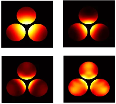
Figure 3 shows an example of a proximity simulation for a simple three-cable based configuration and a uniform cross-sectional current density for the lowest harmonich= 1and where the current is taken to flow in the same direction (in or out of the plane). Figure 3 also shows the PSF, the Magnetic Field Potential and the proximity temperature based on equations (14) and (13), respectively. Each cable is taken to ‘radiate’ a Magnetic Potential Field in the plane which induces a secondary Electric Field in the proximity cable. This secondary Electric Field induces a proximity current density and thus a (square current) proximity tem-perature effect whose field pattern is determined by equation (13). Figure 4 shows the proximity temperatures for higher harmonics h = 3,5,7,9 and illustrates the surface heating that occurs when higher harmonics are considered in terms of the proximity effects generated by the influence of the magnetic field generated by one cable with another. Two results emerge from these simulations that are notable: (i) Lower harmonic proximity temperatures are biased toward the cable (outer) surfaces in local proximity to each other; the proximity temperature exhibits an increased asymmetry as the harmonic order increases, the region of maximum temperature being skewed toward the surfaces in closer proximity to each other. The last point in the above list is explained in terms of the skin effect. However, as the harmonics increase further the heat is distributed on both the surface and the interior of the cable. This effect is due

Fig. 3. A three conductor configuration in the plane (top-left for a grey scale colour map) for a uniform current density using a500×500_regular

Cartesian Grid, the Fresnel Point Spread Function (top-right for a grey scale colour map), the Magnetic Field Potential (bottom-left) given by equation (14) and the proximity temperature (bottom-right) given by equation (13) for

h= 1using the MATLAB ‘Hot’ colour map. In each case, the fields shown are normalised and therefore represents aa two-dimensional numerical field with values between 0 and 1 inclusively. Thus in both the colour maps used, 0 corresponds to Black and 1 corresponds to White.

to the nature of the PSF which generates quadratic phase wavefronts as the value of the harmonic increases. This is not a feature of the conventional skin effect that is based on a model for the penetration on plane wave (for the Electric Field) in a conductor, as illustrated in Section V(B), which is consistent only with regard to a far-field analysis of the Green’s function used to obtain a solution to equations (5).

The effect of multiple cable arrays and the induction temperatures induced in neutral proximity conductors (i.e. conductors with zero primary current density) is easily sim-ulated using equation (13) where the proximity conductivity is taken to be the combination of conductors with and without a primary current densityj(x, y). This is a common problem with regard to the assembly of power cables in cable trays, an example of which is shown in Figure 5. An example is

Fig. 5. Example of a power cable assembly in a conductive cable tray.

shown in Figure 6 for a non-symmetrical array of nine cables supported by a semi-rectangular metal cable tray and where is it clear that:

1) proximity temperature effects are induced in the tray which have proximity temperatures of the order of the cables closest to the tray;

2) the inner cable of the array reaches the highest proxim-ity temperature (for all harmonics) due to its proximproxim-ity to largest number of surrounding cables.

VIII. THREE-DIMENSIONALSIMULATIONS For the three-dimensional case, equations (14) and (13) become

M(x, y, z) =|j(x, y, z)⊗3exp[iα(x2+y2+z2)]|

and

T(x, y, z) = Tp(x, y, z, k) T0k2µ2

=|σp(x, y, z){j(x, y, z)⊗3exp[iα(x2+y2+z2)]} |2 (15)

respectively, where

α(x2_+y2_+z2_{) =} hπ

N2(n 2

x+n2y+n2z)

∆ being taken to define the spatial resolution of a voxel. Three-dimensional simulations are necessary with regard to computing proximity heating effects in high current loading inter-connectors such as illustrated in Figure 2 when radial symmetry can not be assumed. The same principles apply as those used to generate two-dimensional simulations. How-ever, working with a three-dimensional regular grid requires

Fig. 6. Proximity temperature distributions associated with a stack of cables all with the same flow of alternating current (in or out of the plane) housed in a rectangular cable tray which is taken to have the same conductivity as the cables but with no primary (only an induced) current (top-left). The proximity temperature generated by the induced current (in both the cables and tray) are shown for harmonicsh= 11,13,15(from top-right to bottom-right, respectively) using the MATLAB ‘Hot’ colour map. In each case the fields shown are normalised and therefore represents aa two-dimensional numerical field with values between 0 and 1 inclusively.

significantly greater CPU time. Further, voxel modelling system are required to generate the input arrays representing the functions j(x, y, z) and σp(x, y, z) together with voxel

graphical representations to visualise the three-dimensional output numerical fields generated.

Voxel modelling systems such asVoxelogic[6] andVoxel Sculpting[7] allow designers to sculpt without any topolog-ical constraints. These systems include open source produce such as VoxCAD [8] that provides for the inclusion of multiple materials and is therefore ideal for introducing designs based on variations in the conductivity and current density. Systems such asPendix, [9] operate like 2D graphics software while producing 3D models and are therefore ideal for designing structures with a single value of the conduc-tivity, for example, although the application of these systems lies beyond the scope of this paper.

By way of an example, we consider a simplified voxel model of the connecting bars and their (square plate) root given in Figure 2. Figure 7 shows a simple visualisation of this model together with an iso-surface of the corresponding Fresnel PSF for h = 10 using a regular Cartesian grid of 1003_{. Figure 7 also shows the two-dimensional} prox-imity temperature field in the (x, y)-planes for z = 1 and

z = 100 based on equation (15), the three-dimensional convolution process being undertaken using the MATLAB function convn. The results are illustrative of the effect of induction currents generated by a three-dimensional magnetic field associated with a uniform current flowing in a relatively simple but three-dimensional structure.

IX. THERMALDIFFUSIONEFFECTS

Fig. 7. Simplified voxel model of the connecting bars and root given in Figure 2 (top-left) for a uniform current density using100×100×100

regular Cartesian grid and an iso-surface of the three-dimensional Fresnel PSF forh= 10(top-right). The proximity temperature fields are shown for the(x, y)-plane atz= 100andz= 1in the bottom-left and bottom-right images, respectively, using the MATLAB ‘Hot’ colour map.

to the square of the frequency. This temperature profile is the source for a temperature field that will thermally diffuse throughout the regions of compact support. Thus, referring to equation (12), the diffusion equation becomes

D∇2

−_∂t∂

T(r, t) =−S(r), T(r, t= 0) =Ti (16)

whereD is the Thermal Diffusivity of the conductor(s),Ti

is the initial temperature and the Source Function S(r, t)is given by

S(r) =T0

N

X

h=1

T0Phk2hµ2|σp(r)[j(r, k)⊗nexp(iαr2)]|2

(17)

for dimensions n = 1,2 and 3, where Ph is the Power

Spectrum and it is noted thatαis a function ofh. The general solution to equation (16) can be obtained using the Green’s function for the diffusion equation and is given by [10]

T(r, t) =Ti(r)⊗nGn(r, t) +S(r)⊗nGn(r, t)

where

Gn(r, t) =

1 4πDt

n2 exp

−

r2

4Dt

H(t)

and

H(t) = (

1, t >0; 0, t <0.

For the steady state case, the time independent diffusion problem applies for which we are required to solve the Poisson equation

D∇2_{T(r) =}

−S(r)

the two- and three-dimensional solutions to this equation being [10]

T(r) = (

−D−1_lnr⊗

2S(r), r∈(0,1];

+D−1_lnr⊗

2S(r), r∈[1,∞).

and

T(r) = 1

4πDr⊗3S(r, k)

respectively.

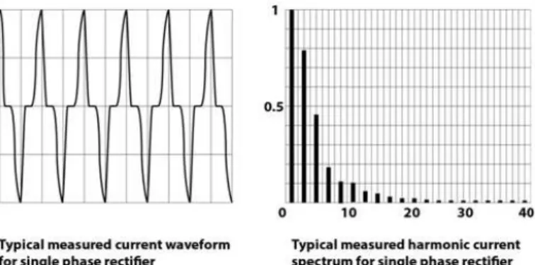
Given that the DiffusivityDof conductive materials used in the construction of power cables is readily available, the principal unknown with regard to the evaluation of equation (17) is the characteristic Power Spectrum. There is no unifying scaling law for the power spectrum associated with harmonic distortion in power cables and the power spectrum can change from one built environment to another depending on the loads and appliances. For example, Figure 8 shows the AC wave form and the corresponding harmonic distortion associated with a single-phase rectifier [11]. Power spectra of this type generate additional heating due to both the skin and proximity effects causing cables to operate at a higher temperature than would be the case without harmonic distortion. The degree of harmonic distortion in the load current determine the degree of additional heating that can occur to which suitable de-rating corrections factor can be applied [12].

Fig. 8. Wave form and harmonic current spectrum for a single-phase rectifier.

X. DISCUSSION

XI. CONCLUSIONS

The model developed in this paper is based on decou-pling Maxwell’s equations through application of a Gauge transformation as detailed in Appendix A. The method of solution is based on a Green’s function solution for the Magnetic Vector Potential given the current density and the application of Ohm’s law. Under this condition the charge density is zero and application of the homogenous boundary conditions on the surface of a conductor allows equation (11) is derived which shows that the proximity temperature is proportional to the square frequency. With regard to the development of a proximity temperature simulation, the key to the approach taken is to consider the Green’s function solution in the Fresnel zone which yields a convolution based model compounded in equation (12).

The simulations are similar in both two- and three-dimensions and in both cases can be used to investigate the proximity heating effects generated at different harmonics. Higher harmonic effects are particularly important in the design of cable arrays and component structures but relies on knowledge of the spectrum of the harmonic components present in the wave form of an AC load current which must be determined experimentally, a priori. Note that in the example simulations presented, the primary current density

j is taken to be uniformly distributed which, in general, will not be the case due to (self-induced) skin effects in the pri-mary conductor(s). Furthermore, the proximity conductivity

σp may be non-uniform and the magnetic permeability µ

may also be expected to change for different elements of a power cable and proximity components. However, within the context of the model presented, these physical aspects are readily incorporated.

One of the goals of the simulator developed is to evaluate the possible presence of ‘hotspots’ in the design of cable configurations and proximal structures for harmonics that are present in the load. Although proximity temperature effects are subject to thermal diffusion, as discussed in Section IX, in the context of the problem considered here, proximity related hotspots represent a continuous source of heat and can therefore be evaluated independently of thermal diffusion processes. As these effects are also present in electrical machines and equipment used in the built environment, in addition to determining harmonic de-rating factors for power cables arranged in different layouts and combinations, the simulator will provide a powerful design tool for a diverse range electrical equipment and machines which contain non-trivial conductor topologies and magnetic circuits.

APPENDIXA: MAXWELL’SEQUATIONS AND THE MAGNETICVECTORPOTENTIAL

The motions of electrons (and other charged particles) give rise to electric and magnetic fields [13], [14]. These fields are described by the following equations which are a complete mathematical descriptions for the physical laws stated for constant electric permittivity ǫ and (constant) magnetic permeabilityµ.

Coulomb’s law

∇ ·E=ρ

ǫ (A.1)

Faraday’s law of induction

∇ ×E=−µ∂B

∂t (A.2)

No free magnetic monopoles exist

∇ ·B= 0 (A.3)

Modified (by Maxwell) Ampere’s law

∇ ×B=ǫ∂E

∂t +j (A.4)

where E is the electric field, B is the magnetic field, j is the current density and ρ is the charge density These equations are used to predict the electric E and magnetic B fields given the charge and current densities (ρ and j respectively) for the case when the material parameters defined byǫandµare constant. The differential operator∇

is defined as follows:

∇ ≡ˆi ∂

∂x+ ˆj ∂ ∂y + ˆk

∂ ∂z

for unit vectors (ˆi,ˆj,kˆ). By including a modification to Ampere’s law, i.e. the inclusion of the ‘displacement current’ termµ∂E/∂t, Maxwell provided a unification of electricity and magnetism compounded in the equations above.

A.1 Linearity of Maxwell’s Equations

Maxwell’s equations are linear because if

ρ1, j1→E1, B1

and

ρ2, j2→E2, B2

then

ρ1+ρ2, j1+j2→E1+E2, B1+B2

where _→ means ‘produces’. This is because the operators

∇·, ∇×and the time derivatives are all linear operators.

A.2 Solution to Maxwell’s Equations

The solution to these equations is based on exploiting the properties of vector calculus and, in particular, identities involving the curl. Taking the curl of equation (A.2), we have

∇ × ∇ ×E=−µ∇ ×∂B ∂t

and using the identity

∇ × ∇ ×E=∇(∇ ·E)− ∇2_E

together with equations (A.1) and (A.4), we get

1

ǫ∇ρ− ∇

2_E=

−µ∂ ∂t

ǫ∂E ∂t +j

or, after rearranging,

∇2_E− 1

c2

∂2_E

∂t2 =

1 ǫ∇ρ+µ

∂j

where

c=_√1 ǫµ

Taking the curl of equation (A.4), using the identity above, equations (A.2) and (A.3) and rearranging the result gives

∇2_B

−_c12

∂2_B

∂t2 =−∇ ×j. (A.6) Equations (A.5) and (A.6) are inhomogeneous wave equa-tions for E and B. These equations are ‘coupled’ to the vector field j (which is related toB). If we define a region of free space where ρ= 0 andj = 0, then both E and B satisfy the equation

∇2_f

− 1 c2

∂2_f

∂t2 = 0.

This is the homogeneous wave equation. One possible solu-tion of this equasolu-tion (in Cartesian coordinates) is

fx=p(z−ct); fy = 0, fz= 0

which describes a wave or distribution p moving along

z at velocity c. Thus, in free space, Maxwell’s equations describe the propagation of an electric and magnetic (or electromagnetic field) in terms of a wave traveling at the speed of light.

A.3 General Solution to Maxwell’s Equations

The solution to Maxwell’s equation in free space is specific to the charge density and current density being zero. We now investigate a method of solution for the general case [15], [16]. The basic method of solving Maxwell’s equations (i.e. finding EandB givenρandj) involves the following:

1) Expressing E and B in terms of two other fields U

andA.

2) Obtaining two separate equations forU andA. 3) Solving these equations for U and A from which E

andB can then be computed. For any vector field A

∇ · ∇ ×A= 0.

Hence, if we write

B=∇ ×A (A.7)

then equation (A.3) remains unchanged. Equation (A.2) can then be written as

∇ ×E=−µ∂ ∂t∇ ×A

or

∇ ×

E+µ∂A ∂t

= 0.

The fieldAis called the Magnetic Vector Potential. For any scalar fieldU

∇ × ∇U = 0

and thus equation (A.2) is satisfied if we write

±∇U =E+µ∂A ∂t

or

E=−∇U −µ∂A

∂t (A.8)

where the minus sign is taken by convention.U is called the Electric Scalar Potential.

Substituting equation (A.8) into Maxwell’s equation (A.1) gives

∇ ·

∇U+µ∂A ∂t

=−ρ_ǫ

or

∇2_U+µ∂

∂t∇ ·A=− ρ

ǫ. (A.9)

Substituting equations (A.7) and (A.8) into Maxwell’s equa-tion (A.4) gives

∇ × ∇ ×A+ǫ∂ ∂t

∇U +µ∂A ∂t

=j

Finally, using the identity

∇ × ∇ ×A=∇(∇ ·A)− ∇2_A we can write

∇2_A

− 1 c2

∂2_A

∂t2 − ∇

∇ ·A+ǫ∂U ∂t

=−j (A.10)

If we could solve equations (A.9) and (A.10) above for U

andAthenEandBcould be computed. The problem here, is that equations (A.9) and (A.10) are coupled. They can be decoupled by applying a technique known as a ‘Gauge Transformation’. The idea is based on noting that equations (A.7) and (A.8) are unchanged if we let

A_→A+∇X

and

U →U−ǫ∂X ∂t

since ∇ × ∇X = 0. If this gauge function X is taken to satisfy the homogeneous wave equation

∇2_X

−_c12

∂2_X

∂t2 = 0 then

∇ ·A+ǫ∂U

∂t = 0 (A.11)

which is called the Lorentz condition. With equation (A.11), equations (A.9) and (A.10) become

∇2_U

−_c12

∂2_U

∂t2 =−

ρ

ǫ (A.12)

and

∇2_A

−_c12

∂2_A

∂t2 =−j (A.13) respectively. These equations are non-coupled inhomoge-neous wave equations and in this paper, the principal equa-tion used to derive a simulaequa-tion for proximity effects is equation (A.13) with equation (A.8) serving to relate the solution forA, via the Green’s function solution to equation (A.13), to the Electric Field E, subject to the conditions that ρ = 0 (appropriate for highly conductive media) and

U = 0 (a consequence of using the homogeneous boundary conditions).

ACKNOWLEDGMENTS

REFERENCES

[1] Cenelec, ‘BS EN 50160:2000’, in Voltage Characteristics of Electricity Supplied by Public Distribution Systems, 2000.

[2] Canelec, ‘BS EN 61000-3-2 Ed.2:2001 IEC 61000-3-2 Ed.2:2000 Electromagnetic Compatibility (EMC)’, in Part 3-2: Limits for Har-monic Current Emissions (Equipment Input Current upto and Including 16 A per Phase), 2001.

[3] IEEE, ‘IEEE Std 519-1992 (USA)’, IEEE Recommended Practices and Requirements for Harmonic Control in Electrical Power Systems’, 1992.

[4] N. R. W. J. Arrillaga,Power System Harmonics, Second Edition ed.: John Wiley and Sons, Ltd, 2003.

[5] S. J. B. Ong and C. YeongJia,An Overview of International Harmonics Standards and Guidelines (IEEE, IEC, EN, ER and STC) for Low Voltage System, Power Engineering Conference, IPEC (2007), 602-607, 2007.

[6] Voxelogic, http://www.voxelogic.com

[7] Voxel Sculpturing http://3d-coat.com/voxel-sculpting/ [8] VoxCad, http://www.voxcad.com/

[9] Pendix, http://home.arcor.de/sercan-san/homepage/sangames/sites/ project pendix.html

[10] G. A. Evans, J. M. Blackledge and P. Yardley,Analytical Solutions to Partial Differential Equations, Springer, 1999.

[11] Gambica (Ed.),Managing Harmonics: A Guide to ENA Engineering Recommendation G5/4-1, Sixth Edition, 2011.

[12] K. O’Connell, J. M. Blackledge, M. Barrett and A. Sung, Cable Heating Effects due to Harmonic Distortion in Electrical Installations, International Conference of Electrical Engineering, World Congress on Engineering (WCE2012), London 4-6 July, IAENG, 928-933, 2012. [13] J. A. Stratton,Electromagnetic Thoery, McGraw-Hill, 1941. [14] P. M. Morse and H. Feshbach, Methods of Theoretical Physics,

McGraw-Hill, 1953.

[15] R. H. Atkin,Theoretical Electromagnetism, Heinemann, 1962. [16] B. I. Bleaney,Electricity and Magnetism, Oxford University Press,

1976.

Professor Jonathan Blackledge holds a PhD in The-oretical Physics from London University and a PhD in Mathematical Information Technology from the Univer-sity of Jyvaskyla. He has published over 200 scientific and engineering research papers including 14 books, has filed 15 patents and has been supervisor to over 200 MSc/MPhil and PhD research graduates. He is the Science Foundation Ireland Stokes Professor at Dublin Institute of Technology where he is also an Honorary Professor and Distinguished Professor at Warsaw University of Technology. He holds Fellowships with leading Institutes and Societies in the UK and Ireland including the Institute of Physics, the Institute of Mathematics and its Applications, the Institution of Engineering and Technology, the British Computer Society, the Royal Statistical Society and Engineers Ireland.

Professor Eugene Coyleis Head of Research Innovation and Partnerships at the Dublin Institute of Technology. His research spans the fields of control systems and electrical engineering, renewable energy, digital signal processing and ICT, and engineering education and has published in excess of 120 peer reviewed conference and journal papers in addition to a number of book chapters. He is a Fellow of the Institution of Engineering and Technology, Engineers Ireland, the Energy Institute and the Chartered Institute of Building Services Engineers, was nominated to chair the Institution of Engineering and Technology (IET) Irish branch committee for 2009/10 and a member, by invitation, of the Engineering Advisory Committee to the Frontiers Engineering and Science Directorate of Science Foundation Ireland, SFI.