The annual ammonia budget of fertilised cut grassland – Part 2: Seasonal variations and compensation point modeling

Biogeosciences, 7, 537–556, 2010 www.biogeosciences.net/7/537/2010/

© Author(s) 2010. This work is distributed under the Creative Commons Attribution 3.0 License.

Biogeosciences

The annual ammonia budget of fertilised cut grassland – Part 2:

Seasonal variations and compensation point modeling

C. R. Flechard1, C. Spirig2, A. Neftel2, and C. Ammann2

1_{INRA, Soils, Agro- and hydro-Systems (SAS) Unit, 65, rue de St.-Brieuc, 35042 Rennes Cedex, France}

2_{Agroscope Reckenholz-T¨anikon ART, Swiss Federal Research Station, Reckenholzstrasse 191, 8046 Z¨urich, Switzerland} Received: 3 September 2009 – Published in Biogeosciences Discuss.: 7 October 2009

Revised: 6 January 2010 – Accepted: 15 January 2010 – Published: 8 February 2010

Abstract. The net annual NH3 exchange budget of a fer-tilised, cut grassland in Central Switzerland is presented. The observation-based budget was computed from semi-continuous micrometeorological fluxes over a time period of 16 months and using a process-based gap-filling proce-dure. The data for emission peak events following the ap-plication of cattle slurry and for background exchange were analysed separately to distinguish short-term perturbations from longer-term ecosystem functioning. A canopy compen-sation point model of background exchange is parameterised on the basis of measured data and applied for the purposes of gap-filling. The data show that, outside fertilisation events, grassland behaves as a net sink for atmospheric NH3with an annual dry deposition flux of−3.0 kg N ha−1yr−1, although small NH3 emissions by the canopy were measured in dry daytime conditions. The median Ŵs ratio in the apoplast

(=[NH+₄]/[H+_{]) estimated from micrometeorological}

mea-surements was 620, equivalent to a stomatal compensation point of 1.3 µg NH3m−3 at 15◦C. Non-stomatal resistance to depositionRw was shown to increase with temperature

and decrease with surface relative humidity, and Rw

val-ues were among the highest published for European grass-lands, consistent with a relatively high ratio of NH3to acid gases in the boundary layer at this site. Since the gross an-nual NH3emission by slurry spreading was of the order of

+20 kg N ha−1yr−1, the fertilised grassland was a net NH3 source of+17 kg N ha−1yr−1. A comparison with the few other measurement-based budget values from the literature reveals considerable variability, demonstrating both the in-fluence of soil, climate, management and grassland type on the NH3budget and the difficulty of scaling up to the national level.

Correspondence to:C. R. Flechard

(chris.flechard@rennes.inra.fr)

1 Introduction

The relative importance of ammonia (NH3) as an atmo-spheric pollutant has increased in Europe over the last two decades. The implementation within the UNECE Conven-tion on Long-Range Transboundary Air PolluConven-tion of the Helsinki and Oslo Protocols on sulphur (1985, 1994), of the Sofia Protocol on nitrogen oxides (1988), and of the Gothenburg Protocol to abate acidification, eutrophication and ground-level ozone (1999), will likely eventually result in NH3 being the main contributor to acidifying deposition (Amann et al., 2005). Other environmental impacts of NH3 deposition include ecosystem eutrophication, loss of biodi-versity as well as direct effects of gaseous NH3on plants, nitrification and leaching of nitrate (NO−₃) to groundwater, ammonium (NH+₄) aerosol formation, and contribution to climate change through deposition-induced N2O emission (Galloway et al., 2003; Erisman et al., 2007).

Grasslands are widely recognised as both sources and sinks of NH3, depending on their fertilisation status, but also on the time of day and season of year. Semi-natural and unfertilised agricultural grasslands have been observed to behave mostly as sinks during night-time and winter, with occasional emissions occurring at noon and in the summer (Hesterberg et al., 1996; Flechard and Fowler, 1998; Mil-ford et al., 2001a; Spindler et al., 2001; Horvath et al., 2005; Wichink Kruit et al., 2007). Intensively managed grasslands, however, are generally net NH3emitters (Plan-taz, 1998; Mosquera et al., 2001; Milford, 2004), with NH3 emissions being triggered or enhanced by management prac-tices such as mineral fertilisation (Bussink et al., 1996; Her-rmann et al., 2001, 2009; Milford, 2004; Mattsson et al., 2009) and manure application (Mosquera et al., 2001); by grazing animals (Plantaz, 1998; Milford, 2004) or even large numbers of birds (Mosquera et al., 2001); by the cutting of grass and the decomposition of left-over or senescent plant

material in a leaf litter (Burkhardt et al., 2009; Milford, 2004; Mannheim et al., 1997); and generally, by an elevated plant nitrogen (N) status resulting in a compensation point being higher than the ambient concentration, leading to NH3loss through stomata (Mattsson et al., 2009; Massad et al., 2008; Sutton et al., 1998; Farquhar et al., 1980).

Over grazed or fertilised agro-ecosystems, the continu-ous or discontinucontinu-ous supply of animal excreta, urine, ma-nure or slurry, or synthetic nitrogen (N)-containing fertilis-ers, leads to both direct, short-term NH3 emissions follow-ing the application, and indirect and longer-term plant- or soil-mediated exchange by raising the N-status of the system (Riedo et al., 2002; Herrmann et al., 2001). In the case of fertiliser application to non-grazed systems, emission bursts or “events” may be considered as short-lived disturbances of the system, which gradually reverts to a state of equilib-rium or “background” exchange with the atmosphere. Un-like background exchange, which exhibits rather regular di-urnal and seasonal patterns controlled by meteorology and grassland growth and phenology, peak emissions from fer-tiliser application are characterized by strong asymmetrical dynamics over a few days with successive pulses of decreas-ing strength. The emission flux and NH3 surface concen-tration thus decrease rapidly, broadly following an exponen-tial decay curve (Spirig et al., 2010; G´enermont et al., 1998; Thompson and Meisinger, 2004) back to values close to those observed prior to fertilisation.

Most micrometeorological measurements to date of the surface/atmosphere exchange of NH3over intensively man-aged grassland have been carried out within the framework of relatively short campaigns of typically a few weeks (e.g. the GRAMINAE Braunschweig campaign, Sutton et al., 2008, 2009). In contrast, long-term monitoring studies that encom-pass the full range of management activities (grazing, cut-ting, fertiliser applications) as well as the whole annual veg-etative cycle, are scarce and largely limited to the oceanic climatic zone of NW Europe (Plantaz, 1998; Mosquera et al., 2001; Milford, 2004). The results indicate that the gross emission from all processes in fertilised grassland, including emissions from fertilisation, grazing and cutting, can make a significant contribution to national NH3 emissions (Mil-ford, 2004). The annual NH3 budgets reported at the in-tensively managed grassland site of Schagerbrug and at the semi-natural site of Oostvaardersplassen in Northern lands (Mosquera et al., 2001), at Zegveld in Central Nether-lands (Plantaz, 1998), and at Easter Bush in Southern Scot-land (Milford, 2004), all show management event-dominated emission budgets that are somewhat offset by dry deposi-tion during a large part of the year. Only one of these sites (Schagerbrug) was ungrazed, and very few measurement-based estimates of the annual NH3budget for fertilised, cut grasslands are available in the literature.

In this paper we report a year-long, semi-continuous time series of field measurements of NH3 exchange over fer-tilised cut grassland in a continental climate (Switzerland).

To describe the exchange mechanistically and fill gaps in the flux time series, the single-layer canopy compensation point modeling framework of Sutton et al. (1998) is param-eterised and applied in background conditions. The extent to which a grassland canopy may be satisfactorily approxi-mated by a single-layer model for the purpose of simulating background NH3exchange is discussed. The data are used to derive parameterisations for single-layer exchange frame-works that are widely applied in regional atmospheric trans-port and deposition models (Sorteberg and Hov, 1996; Smith et al., 2000; Simpson et al., 2003).

The case of strong NH3 emissions after cattle slurry ap-plication is treated separately, as processes leading to NH3 evolution from liquid manure applied onto soils are differ-ent altogether from those regulating background exchange (e.g. G´enermont and Cellier, 1997). The full description of flux measurements during slurry “events” and the uncertainty introduced by advection and footprint errors (Loubet et al., 2001; Neftel et al., 2008) are treated in the companion paper by Spirig et al. (2010).

The main objectives of this paper were therefore 1) to study seasonal variations in NH3exchange over fertilised cut grassland; 2) to identify key parameters driving background ammonia exchange; 3) to parameterise a canopy compensa-tion point model (Sutton et al., 1998) for this grassland site; and 4) to calculate an annual, observation-based NH3budget based on both background and peak emission fluxes.

2 Materials and methods

2.1 Site description

C. R. Flechard et al.: The ammonia budget of fertilised grassland 539 2.2 Micrometeorological measurements

Semi-continuous micrometeorological NH3 flux measure-ments took place from July 2006 through October 2007, with interruptions in winter (December to February) and in late summer 2007. Turbulent fluxes were determined for every half-hour period using the aerodynamic gradient method or AGM (Monteith and Unsworth, 1990) from the product of friction velocity u∗, measured by an ultrasonic anemome-ter according to CarboEurope-IP guidelines (Ammann et al., 2007), and of the stability-corrected, vertical gradient in NH3 concentration (χ):

Fχ= −ku∗

∂χ

∂ ln(z−d)−ψH z−_Ld

(1)

wherezis height above ground,dis the displacement height,

k is von Karman’s constant (0.41), L is Monin-Obukhov length andψH is the integrated stability function for heat

and trace gases (for details see Spirig et al., 2010). Ammo-nia concentrations were measured at two heights above the canopy using AiRRmonia detectors (Mechatronics, Hoorn, The Netherlands; http://www.mechatronics.nl; see also Eris-man et al., 2001).

During periods when gradient-flux measurements were not running, NH3 concentration was measured as monthly averages at one height (1.5 m above ground) using a DELTA system (DEnuder for Long-Term Ammonia; Sutton et al., 2001). Here, NH3 was captured by the citric acid-coated inner surface of glass denuders after lateral molecular dif-fusion in a laminar flow of sampled ambient air, following the method by Ferm (1979). The monthly mean concentra-tion was determined after extracconcentra-tion of the denuder follow-ing exposure in the field and chemical analysis of the NH+₄ concentration performed using an AMFIA (AMmonia Flow Injection Analysis) system (ECN, Petten, The Netherlands). These data were part of a wider network of 56 DELTA mon-itoring sites across Europe within the framework of the Ni-troEurope project (Sutton et al., 2007; Tang et al., 2009). The Oensingen DELTA NH3data were thus used in the gap-filling procedure for the calculation of the annual NH3 ex-change budget at this site (see Sect. 2.4).

2.3 Inferences from micrometerological measurements and compensation point modeling

2.3.1 Basic principles of inferential modeling

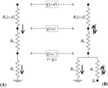
The surface/atmosphere transfer of NH3 may be conceptu-alized as an electrical analogue within a network of resis-tances characterizing transfer pathways through the canopy and between the surface and the atmosphere (Monteith and Unsworth, 1990; Thom, 1975). For depositing trace gases, micrometeorological flux measurements have traditionally provided experimental estimates of the canopy resistanceRc

as the difference between the inverse deposition velocityV_d−1

(equal to the total resistance to deposition), and the sum of at-mospheric aerodynamic and pseudo-laminar boundary layer resistances (Ra+Rb) (Garland, 1977) (see Fig. A1a). Dry

de-position models seek to predictRc from environmental and

ecosystem drivers, with the objective of inferring the depo-sition flux Fχ as the product of concentration and

deposi-tion velocity, assuming that the canopy concentradeposi-tion is zero. Indeed, most regional atmospheric transport and deposition models still use a deposition-only,Rc−Vdapproach for NH3

(Simpson et al., 2003; Zhang et al., 2003; Erisman et al., 1994).

However, the soil/vegetation/atmosphere exchange of NH3 has long been shown to be clearly bi-directional (e.g. Dabney and Bouldin, 1990; Sutton et al., 1995a), as there exists a non-zero bulk canopy NH3 potential χ{z′₀} (see Fig. A1b), allowing both deposition and emission to oc-cur depending on the ambient atmospheric concentration

χ{z−d}. This is due to the occurrence of dissolved NH3 and NH+₄ in the apoplastic fluid of leaves (Farquhar et al., 1980), characterised by a stomatal compensation point (χs),

in leaf surface water films, and in the decaying plant material of a leaf litter on the ground (Nemitz et al., 2000; Mannheim et al., 1997). Second generation models based on the canopy compensation point (χc) concept (Sutton et al., 1998; Smith

et al., 2000; Wu et al., 2009) have thus been developed. The potentialsχc andχ{z′₀}are conceptually equivalent, though

the former is taken in this paper to represent a model (predic-tive) formalization of the latter, which is experimentally es-timated from micrometeorological flux data. Both terms are effectively notional average (bulk) canopy concentrations. 2.3.2 The single-layer canopy compensation point

model

The Sutton et al. (1998) single-layerχc model, also known

as theχs−Rw model (Fig. A1b), predicts the net NH3

ex-change as resulting from 1) bi-directional flux through plant stomates, impeded by the stomatal resistanceRs, and 2) the

capture by leaf cuticles, surface water layers and other non-stomatal surfaces, collectively through the resistance Rw.

The net exchange flux is modelled as:

Fχ=

χc−χ{z−d}

Ra{z−d} +Rb

(2) where χ and Ra are evaluated at a reference height z−d

(=1 m in the present study). Sutton et al. (1998) show that the resolution of the resistance network yieldsχcas:

χc=

χ{z−d}

(Ra{z−d}+Rb)+ χs Rs

1

(Ra{z−d}+Rb)+

1

Rs+

1

Rw

≡χz′₀ (3)

The resistancesRa andRbare relatively well characterised

and readily calculated from micrometeorological measure-ments (e.g. Monteith and Unsworth, 1990; Garland, 1977):

Ra(z−d)=

1

ku∗

ln

_z−d

z0

−ψH

_z−d

L

+ψH

z₀

L

(4) and

Rb=

1.45 z0u∗

ν

0.24 ν D

0.8

u∗

(5) wherez0 is the roughness length,d+z0 being the notional height of momentum exchange and theoretical zero wind-speed,νis the kinematic viscosity of air andDis the molec-ular diffusivity of NH3in air.

2.3.3 Parameterisations forRs,Rwandχs

Micrometeorological flux measurements made in back-ground conditions at Oensingen were analysed in such a way as to derive the remaining unknowns in Eq. (3) i.e.Rs,Rw

andχs, which were inferred from measured NH3and water

vapour concentrations and fluxes. The first step is the calcu-lation of the bulk canopy NH3concentrationχ{z′₀}, which is given by a straightforward extrapolation from the reference height (z−d) down toz0’:

χz′₀ =χ{z−d} +Fχ(Ra{z−d} +Rb) (6)

The bulk stomatal resistance (Rs) was evaluated for H2O

from the measured latent heat flux (λE), which was a rou-tine output of the CarboEurope-IP eddy covariance (EC) flux monitoring programme, alongsideu∗, sensible heat flux (H)

and CO2exchange (Ammann et al., 2007). In dry, daytime conditions most of the evapotranspiration fluxEmay be as-sumed to issue from stomata, with close to negligible con-tributions from soil and leaf surface evaporation. Thus the vapour pressure deficit (vpd) at heightz′₀bears a direct rela-tionship toEandRs such that (Thom, 1975; Monteith and

Unsworth, 1990):

Rs{H2O} =

ρε p

vpd

E =

ρε p

esatT z₀′ −ez₀′

E (7)

whereρis air density,pis atmospheric pressure,εis the ra-tio of the molecular weight of water to the mean molecular weight of dry air (18/29), andesat{T (z₀′)}ande{z′₀}are the saturation water vapour pressure and actual vapour pressure at heightz₀′. The surface potentialsT{z₀′}ande{z₀′}are esti-mated using a similar extrapolation to that for NH3(Eq. 6):

T

z′₀ =T{z−d} + H

ρCp

(Ra{z−d} +Rb) (8)

withCpthe specific heat capacity of air, and,

ez′₀ =e{z−d} +pE

ρε(Ra{z−d} +Rb) (9)

As stomatal resistance could only be evaluated experimen-tally in dry conditions, a light-response parameterisation of

Rs, which has been applied extensively in the flux modeling

literature (Baldocchi et al., 1987; Hicks et al., 1987; Erisman

et al., 1994; Nemitz et al., 2001; Zhang et al., 2003), was used whenever no measuredRs was available, e.g. after rain

or in the early morning before dew had evaporated:

Rs{NH3} =Rs,min

1+b

′

Ip

/(fefwfTfs) (10)

Here,Ipis the photosynthetic radiation intensity,b′is an

em-pirical constant,Rs,minis the minimum value ofRs and the

correction factorsfe, fw andfT account for the effects of

increasing vpd, plant water stress and temperature, respec-tively (Jarvis, 1976), althoughfw was actually set to 1 in the

absence of leaf water potential measurements. The stomatal resistance for NH3differs from that for H2O by the ratio of their respective molecular diffusivities (Hicks et al., 1987; Wesely, 1989), which is accounted for in the last correction factorfs. TheRs,minandb′parameters were fitted indepen-dently and separately for each growth phase on both INT and EXT fields, as was the parameterbeneeded in the calculation

of the vpd stress factor (fe=1−be·vpd; Hicks et al., 1987).

Note thatRsin Eq. (10) is expressed on a unit leaf area basis;

the bulk (canopy) stomatal resistance is scaled by the inverse leaf area index (LAI−1).

From the knowledge ofχ{z′₀}andRs, the termsχsandRw

may be approached separately. In a similar fashion to previ-ous studies (Nemitz et al., 2001, for a review), the non stom-atal resistanceRw, also termedRext(Erisman et al., 1994) or

Rcut(Hicks et al., 1987), was derived from night-time mea-surements, whenRsmay be assumed to be much larger than

Rw so that Eq. (3) simplifies to:

Rw(night)∼=(Ra{z−d} +Rb)

χ

z0′

χ{z−d} −χ{z0′}

(11) It should be noted that 1)Rw may only be evaluated in this

fashion if χ (z−d)>χ{z′₀}, i.e. only in the case of deposi-tion, lestRwbe negative; and 2)Rwis essentially equivalent,

during night-time, toRc calculated as the residual between

Rt and (Ra+Rb) in a canopy resistance framework. The

use of a high night-time value forRs (e.g. 5000 s m−1)

us-ing Eq. (3), instead of the simplified Eq. (11), yields similar results forRw.

In theory,χs could be obtained from Eq. (3) if

experimen-tal estimates ofχ{z′₀},RsandRware available, but the

com-bined potential error or noise in these terms would result in a high uncertainty for individual values of χs. An option

sometimes preferred (Flechard et al., 1999; Spindler et al., 2001; Nemitz et al., 2001), and also used here, consists in se-lecting individual flux measurement runs in dry conditions, when the exchange switches from deposition to emission, or vice versa, i.e. the net flux is close to zero. Under the hy-potheses 1) that stomata are open, 2) thatRw is very large,

and 3) that therefore stomatal exchange may reasonably be expected to represent by far the major pathway, thenχs may

C. R. Flechard et al.: The ammonia budget of fertilised grassland 541 termedŴs, which characterizes the emission potential of the

plant leaves, though normalized for the effect of temperature on NH3solubility in water, may be inferred from (Flechard et al., 1999):

Ŵs=

χs×10−9

104.1218−4507/T{z0′} χsin ppb andT{z

′

0}inK (12) 2.4 Gap-filling and NH3budget

2.4.1 Data management

The annual budget of NH3exchange was calculated by inte-grating background exchange and fertiliser-induced emission peaks separately, which has been done for N2O exchange at the same site (Flechard et al., 2005). The background vs. fertiliser events split has the merit of showing what the NH3 budget might have been in the absence of fertiliser applica-tions. It is acknowledged, however, that fertilisation alters the N status of plants (total N, substrate N, and apoplastic NH+₄ concentrations) (Riedo et al., 2002), and in the longer term affects background exchange through a raisedχs. A

fur-ther justification for the split lies in the necessarily dynamic modeling of NH3 emission by slurry applied to soil, with a rapid depletion of an initial NH+₄ pool (e.g. G´enermont and Cellier, 1997), as opposed to the essentially staticχs−Rw

approach applied for background exchange. In the latter, the apoplastic NH+₄ content is considered in a first approxima-tion to be in a buffered equilibrium with the soil-plant sys-tem and roughly constant over longer time scales, although this has been disputed (Herrmann et al., 2009; Mattsson et al., 2009).

The measured surface concentrationχ{z′₀}was the crite-rion used to determine the end of the fertiliser-induced “dis-turbance”, and the resumption of background conditions; the determination of the threshold is detailed in the “Results” section. Flux integration and annual budget calculation could be sensitive to this threshold to the extent that parameterisa-tions derived forχs andRw from measured data are less

in-fluenced by concentrations and processes in the slurry layer, and more by plant physiology, canopy cycling and meteo-rological conditions, if the time elapsed since fertilisation is longer. By selecting data appropriately, one may hope to de-rive parameterisations that are suitable for background ex-change at this (and other) site(s).

2.4.2 Cumulative fluxes for background exchange

Two methods were considered for deriving cumulative monthly, seasonal or annual budgets from the semi-continuous time series of measured half-hourly NH3fluxes:

1) Arithmetic mean diurnal cycles of measured fluxes were computed for each month, leaving out data from fer-tiliser events as defined above, and the total monthly background flux was calculated by scaling up from the average flux and the number of background days in

each month. This is statistically the least-biased esti-mate, provided that flux data coverage is high enough (e.g.>50%) and that gaps in the dataset are evenly dis-tributed over time of day and season of year. How-ever, experience has shown at this site (Ammann et al., 2007) that many (40%) night-time fluxes have to be rejected because of low wind speeds (<1 m s−1) and breakdown of turbulence, which are not conducive to satisfactory flux-gradient or EC measurements. Further, there were no flux measurements during certain indi-vidual months (January, February and September 2007), and other months with reduced flux data coverage, pre-cluding the calculation of a reliable annual budget on the basis of monthly fluxes.

2) The time series of actual (measured) NH3 fluxes was gap-filled using theχs−Rwcanopy compensation point

model parameterised specifically for this site (Sect. 2.3), and the cumulative flux was obtained directly from the gap-filled 30-min time series. Inferential model-ing requires the knowledge of NH3 concentration at one height and of standard meteorological data such as air temperature, global radiation, relative humidity, and windspeed (oru∗ and H whenever available). During

brief periods (a few hours to a few days) of interrup-tion of the AiRRmonia monitors, NH3concentration for each missing half-hour was taken from the mean diur-nal course of NH3during the month. For extended peri-ods (>1 month) of AiRRmonia downtime, the monthly (mean) NH3concentration as measured by the DELTA system was used as input to the model.

Method 2) was deemed the least-biased method, and there-fore used for budget calculations, primarily because of the lack of flux measurements in night-time and stable condi-tions (thermal stratification) and in winter. Method 1) (scal-ing up from mean diurnal cycles) was nonetheless applied to calculate monthly fluxes for the purpose of comparison with method 2) (measured and model gap-filled).

2.4.3 Time integration of manure-induced emission fluxes

Emission fluxes measured by the AGM after slurry applica-tion were first corrected to account for errors arising from the horizontal advection of NH3on the field (Loubet et al., 2001) and fetch restrictions (Neftel et al., 2008). By applying the Kormann-Meixner footprint model (Kormann and Meixner, 2001; Neftel et al., 2008) for each half-hourly measurement, Spirig et al. (2010) showed that the AGM underestimated the true (surface) emission fluxes at this site by on average 34% (range: 14–59%), and measured AGM fluxes were cor-rected accordingly. The FIDES model (Flux Interpretation by Dispersion and Echange over Short range) by Loubet et al. (2001) was shown to yield comparable results.

To fill data gaps in the time series of footprint-corrected fluxes during slurry events, an empirical estimate of the canopy potentialχ{z₀′}was used as a predictor of the emis-sion strength. Since ambient NH3 concentration measure-ments at the reference height were available most of the time, as were the standard meteorological variables required to compute estimates ofRaandRb, fluxes could be approached

from the potential difference betweenz₀′ and (z−d) and the sum of atmospheric resistances (Eq. 2). The procedure is de-scribed in detail in Spirig et al. (2010).

3 Results

3.1 Seasonal patterns in measured fluxes and stomatal resistance

The overall picture of NH3exchange from July 2006 through October 2007 is dominated by sharp and relatively short-lived emission peaks induced by six applications of cattle slurry onto the INT plot, which took place in July, Septem-ber and OctoSeptem-ber 2006, and in April, July and OctoSeptem-ber 2007 (Fig. 1). Individual (half-hourly) measured fluxes reached values above +50 µg NH3m−2s−1 (or 1.2 kg N ha−1hr−1) during the first few hours following the spreading of liquid manure onto short (<10 cm) grassland, but the emission was usually reduced to a few 100 ng NH3m−2s−1within a few days of fertilising. For the rest of each grass growth phase until the next cut, background exchange on the INT field was either dominated by deposition (negative fluxes), as in 2006, or characterised in 2007 by bi-directional fluxes mostly in the range −100 to+100 ng NH3m−2s−1 (Fig. 1). The fluxes measured on the EXT field during two short spells (6 d in July 2006 and 16 d in September 2006) were similar in mag-nitude to background fluxes on the INT field, with mostly de-position to the canopy and few emission fluxes greater than

+100 ng NH3m−2s−1. Grass cuts do not appear to have led to enhanced NH3emissions on either field on any occasion during the first 2–3 d when grass lay drying on the ground or was being processed into hay or silage.

Bulk stomatal resistance, derived from EC water vapour flux measurements (Eq. 7) in dry daytime conditions, sponded as expected to grass cuts and the subsequent re-growth, mirroring temporal changes in LAI (Fig. 1, bottom frames). There were also signs in the second half of July 2006 of heat and water stresses, leading to elevated transfer resistances. ModelledRs (Eq. 10) is shown alongside

mea-sured values; fitted parameter values forRs,min,b′andbe

av-eraged 57 s m−1, 97 W m−2and 0.24 kPa−1on the INT field, and 46 s m−1, 92 W m−2 and 0.13 kPa−1 on the EXT field, respectively.

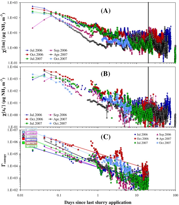
During the transition phase following each slurry event, when NH3 fluxes and concentrations gradually reverted to pre-fertilisation levels, the ambient NH3 concentration

χ{1 m} declined much more rapidly than did the canopy

concentrationχ{z′₀}. Within 2–5 d following the spreading of liquid manure,χ{1 m}had stabilised at background lev-els (Fig. 2a), albeit with typical diurnal variations, whereas the time course of χ{z′₀} clearly shows a much longer-lasting memory effect, following the initial surge upwards of 1000 µg NH3m−3. A visual analysis of Fig. 2b suggests that the effect of the applied slurry on the canopy concentration wears off only after 10–20 d. A threshold of 20 d was thus chosen for all events to distinguish background conditions from fertilisation events.

Figure 2c further illustrates the exponential decay over time of the emission potential of the canopy following spreading, characterised by the bulk [NH+₄]/[H+] ratio of the surface (termedŴcanopy) that one may derive from estimated

χ{z₀′}using Eq. (12). The Ŵcanopy term is initially domi-nated by the manure layer lying on leaves and soil, rather than by the apoplast potential Ŵs. The linear regressions

for the 6 spreading events of log(Ŵcanopy) vs. log(time) are broadly consistent with the initial values ofŴslurry, calculated from the chemical analysis of tank slurry and ranging from 8.5×105to 6.3×106, with slurry [NH+₄] ranging from 0.057 to 0.104 mol l−1, and pH ranging from 7.1 to 7.9 (Spirig et al., 2010).

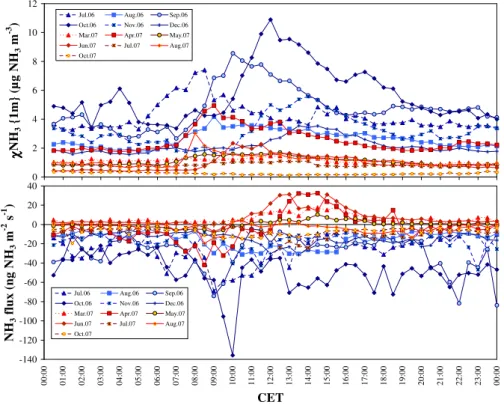
The analysis of mean diurnal cycles in ambient NH3 con-centrations and fluxes for each month of the monitoring pe-riod (background conditions only) reveals key aspects of the combined meteorological and plant physiological control of NH3exchange (Fig. 3). Diurnal concentration profiles typi-cally showed an asymmetrical morning peak during the sum-mer months in 2006, with a sharp rise peaking at around 08:00 CET in July, 09:00 in August, 10:30 in September, followed by a slow decline until around 20:00, and no vari-ations until sunrise the next morning (Fig. 3, top frame). In 2007, the concentrations also peaked asymmetrically in the morning in April, June and August. By contrast, the diurnal variation was more akin to a sine wave with smoother varia-tions in October, November and December 2006 and March, May and July 2007, with a daily maximum centered around noon or early afternoon and a night-time minimum. Con-centrations were considerably higher in 2006 than in 2007, peaking at 10 µg m−3during the day, with night-time values between 2 and 4 µg m−3for much of the second half of 2006, while in 2007 concentrations reached only 4 µg m−3daytime maxima and were otherwise below 2 µg m−3for much of the year.

As a result, diurnal flux patterns (Fig. 3, bottom frame) in-dicate predominant deposition throughout the day in 2006, consistent with ambient concentrations being higher than the canopy compensation point, while there were systematic daytime emissions (10:00–18:00 CET) in spring and early summer 2007, consistent with χc being higher than

C.R. Flechardet al.:The ammonia budget offertilised grassland 543 -1 0 0 0 0 0 1 0 0 0 0 2 0 0 0 0 3 0 0 0 0 4 0 0 0 0 5 0 0 0 0 6 0 0 0 0 7 0 0 0 0 8 0 0 0 0 9 0 0 0 0 06 06 06 06 06 06 06 06 06 06 06 06 06 06 06

NH3 Flux (ng NH3 m

-2

s-1)

0 2₀ 4₀ 6₀ 8₀ 1₀

0 120 140 160 180 200

Slurry application (kg N ha-1)

N H 3 fl u x IN T N H 3 fl u x E X T S lu rr y a p p lic a tio n IN T -1 0 0 0 -8 0 0 -6 0 0 -4 0 0 -2 0 0 0 2 0 0 4 0 0 6 0 0 8 0 0 1 0 0 0 06 06 06 06 06 06 06 06 06 06 06 06 06 06 06

NH3 Flux (ng NH3 m

-2

s-1)

0 2₀ 4₀ 6₀ 8₀ 1₀

0 120 140 160 180 200

Slurry application (kg N ha-1)

N H 3 fl u x IN T N H 3 fl u x E X T S lu rr y a p p lic at io n IN T

0 50

1 0 0 1 5 0 2 0 0 2 5 0 3 0 0 3 5 0 4 0 0 4 5 0 5 0 0 01.06.06 16.06.06 01.07.06 16.07.06 31.07.06 15.08.06 30.08.06 14.09.06 29.09.06 14.10.06 29.10.06 13.11.06 28.11.06 13.12.06 28.12.06

Rs H2O (s m

-1 ) M ea su re d R s I N T M o d el ed R s IN T M ea su re d R s E X T M o d el ed R s E X T C u t I N T C u t E X T -1 0 0 0 0 0 1 0 0 0 0 2 0 0 0 0 3 0 0 0 0 4 0 0 0 0 5 0 0 0 0 6 0 0 0 0 7 0 0 0 0 8 0 0 0 0 9 0 0 0 0 06 06 06 06 06 06 06 06 06 06 06 06 06 06 06

NH3 Flux (ng NH3 m

-2

s-1)

0 2₀ 4₀ 6₀ 8₀ 1₀

0 120 140 160 180 200

Slurry application (kg N ha-1)

N H 3 fl u x IN T N H 3 fl u x E X T S lu rr y a p p lic a tio n IN T -1 0 0 0 -8 0 0 -6 0 0 -4 0 0 -2 0 0 0 2 0 0 4 0 0 6 0 0 8 0 0 1 0 0 0 06 06 06 06 06 06 06 06 06 06 06 06 06 06 06

NH3 Flux (ng NH3 m

-2

s-1)

0 2₀ 4₀ 6₀ 8₀ 1₀

0 120 140 160 180 200

Slurry application (kg N ha-1)

N H 3 fl u x IN T N H 3 fl u x E X T S lu rr y a p p lic at io n IN T

0 50

1 0 0 1 5 0 2 0 0 2 5 0 3 0 0 3 5 0 4 0 0 4 5 0 5 0 0 01.06.06 16.06.06 01.07.06 16.07.06 31.07.06 15.08.06 30.08.06 14.09.06 29.09.06 14.10.06 29.10.06 13.11.06 28.11.06 13.12.06 28.12.06

Rs H2O (s m

-1 ) M ea su re d R s I N T M o d el ed R s IN T M ea su re d R s E X T M o d el ed R s E X T C u t I N T C u t E X T -1 0 0 0 0 0 1 0 0 0 0 2 0 0 0 0 3 0 0 0 0 4 0 0 0 0 5 0 0 0 0 6 0 0 0 0 7 0 0 0 0 8 0 0 0 0 9 0 0 0 0 07 07 07 07 07 07 07 07 07 07 07 07 07 07 07 07 07

NH3 Flux (ng NH3 m

-2

s-1)

0 2₀ 4₀ 6₀ 8₀ 1₀

0 1 2 0 1 4 0 1 6 0 1 8 0 2 0 0

Slurry application (kg N ha-1)

N H 3 fl u x IN T S lu rr y a p p lic a tio n IN T -1 0 0 0 -8 0 0 -6 0 0 -4 0 0 -2 0 0 0 2 0 0 4 0 0 6 0 0 8 0 0 1 0 0 0 07 07 07 07 07 07 07 07 07 07 07 07 07 07 07 07 07

NH3 Flux (ng NH3 m

-2

s-1)

0 2₀ 4₀ 6₀ 8₀ 1₀

0 1 2 0 1 4 0 1 6 0 1 8 0 2 0 0

Slurry application (kg N ha-1)

N H 3 fl u x IN T S lu rr y a p p lic at io n IN T

0 50

1 0 0 1 5 0 2 0 0 2 5 0 3 0 0 3 5 0 4 0 0 4 5 0 5 0 0 01.03.07 16.03.07 31.03.07 15.04.07 30.04.07 15.05.07 30.05.07 14.06.07 29.06.07 14.07.07 29.07.07 13.08.07 28.08.07 12.09.07 27.09.07 12.10.07 27.10.07

Rs H2O (s m

-1 ) M ea su re d R s IN T M o d el ed R s I N T C u t I N T -1 0 0 0 0 0 1 0 0 0 0 2 0 0 0 0 3 0 0 0 0 4 0 0 0 0 5 0 0 0 0 6 0 0 0 0 7 0 0 0 0 8 0 0 0 0 9 0 0 0 0 07 07 07 07 07 07 07 07 07 07 07 07 07 07 07 07 07

NH3 Flux (ng NH3 m

-2

s-1)

0 2₀ 4₀ 6₀ 8₀ 1₀

0 1 2 0 1 4 0 1 6 0 1 8 0 2 0 0

Slurry application (kg N ha-1)

N H 3 fl u x IN T S lu rr y a p p lic a tio n IN T -1 0 0 0 -8 0 0 -6 0 0 -4 0 0 -2 0 0 0 2 0 0 4 0 0 6 0 0 8 0 0 1 0 0 0 07 07 07 07 07 07 07 07 07 07 07 07 07 07 07 07 07

NH3 Flux (ng NH3 m

-2

s-1)

0 2₀ 4₀ 6₀ 8₀ 1₀

0 1 2 0 1 4 0 1 6 0 1 8 0 2 0 0

Slurry application (kg N ha-1)

N H 3 fl u x IN T S lu rr y a p p lic at io n IN T

0 50

1 0 0 1 5 0 2 0 0 2 5 0 3 0 0 3 5 0 4 0 0 4 5 0 5 0 0 01.03.07 16.03.07 31.03.07 15.04.07 30.04.07 15.05.07 30.05.07 14.06.07 29.06.07 14.07.07 29.07.07 13.08.07 28.08.07 12.09.07 27.09.07 12.10.07 27.10.07

Rs H2O (s m

1.E-01 1.E+00 1.E+01 1.E+02 1.E+03

χχχχ

{1

m

}

(µ

g

N

H3

m

-3 )

Jul.2006 Sep.2006 Oct.2006 Apr.2007 Jul.2007 Oct.2007

1.E-01 1.E+00 1.E+01 1.E+02 1.E+03 1.E+04

χχχχ

{z

0

'}

(

µ

g

N

H3

m

-3 )

Jul.2006 Sep.2006 Oct.2006 Apr.2007 Jul.2007 Oct.2007

1.E+02 1.E+03 1.E+04 1.E+05 1.E+06 1.E+07

0.01 0.1 1 10 100

Days since last slurry application

ΓΓΓΓca

n

o

p

y

Jul.2006 Sep.2006

Oct.2006 Apr.2007

Jul.2007 Oct.2007

Γ = 2401825 Γ = 3218664

Γ = 1841789 Γ = 853535 Γ = 6326257 Γ = 4539018

(A)

(B)

(C)

Fig. 2. Temporal dynamics of NH3 concentration following cattle slurry spreading, (A) at the reference height in the surface layer

(z−d=1 m);(B)at canopy levelχ{z′₀}; and(C)bulk canopy emission potentialŴcanopy, derived fromχ{z′₀}, for 6 fertilisation events. Initial values ofŴslurryare shown in (C) for comparison with subsequent micrometeorological estimates ofŴcanopyand the log-log

regres-sion thereof vs. time elapsed. The vertical line at day 20 is the arbitrary threshold chosen to distinguish emisregres-sion events from background exchange.

however clear indicators that over the whole year, the grass-land canopy was a net sink in background conditions.

3.2 Parameterisation of the external leaf surface resistance

Values of Rw estimated during night-time according to

Eq. (11) showed as expected a clear relationship to surface relative humidity (RH{z′₀}) (Fig. 4, top frame), as water films

on leaf cuticles, stems and other non-stomatal surfaces in the canopy are known sinks for atmospheric NH3 (Flechard et al., 1999). The shape of the relationship to RH{z′₀}was ap-proximated to an exponential decay with lowestRwvalues at

100% relative humidity, analogous to the form suggested by Sutton et al. (1998):

Rw=Rw,min×expα×(100−RH{z

′

C. R. Flechard et al.: The ammonia budget of fertilised grassland 545

0 2 4 6 8 10 12

χχχχ

N

H3

{

1

m

}

(µ

g

N

H3

m

-3 )

Jul.06 Aug.06 Sep.06 Oct.06 Nov.06 Dec.06 Mar.07 Apr.07 May.07 Jun.07 Jul.07 Aug.07 Oct.07

-140 -120 -100 -80 -60 -40 -20 0 20 40

0

0

:0

0

0

1

:0

0

0

2

:0

0

0

3

:0

0

0

4

:0

0

0

5

:0

0

0

6

:0

0

0

7

:0

0

0

8

:0

0

0

9

:0

0

1

0

:0

0

1

1

:0

0

1

2

:0

0

1

3

:0

0

1

4

:0

0

1

5

:0

0

1

6

:0

0

1

7

:0

0

1

8

:0

0

1

9

:0

0

2

0

:0

0

2

1

:0

0

2

2

:0

0

2

3

:0

0

0

0

:0

0

CET

N

H3

f

lu

x

(

n

g

N

H3

m

-2 s -1 )

Jul.06 Aug.06 Sep.06 Oct.06 Nov.06 Dec.06 Mar.07 Apr.07 May.07 Jun.07 Jul.07 Aug.07 Oct.07

Fig. 3.Mean diurnal variations of NH3concentration (top) and exchange flux (bottom) in background conditions (all data measured within

the 20-d period following slurry applications were removed from the dataset). CET: Central European Time.

0 200 400 600 800 1000 1200 1400

50 55 60 65 70 75 80 85 90 95 100

RH{z0'} (%) Rw

N

H3

(

s m

-1 )

T<10°C 10<T<15°C T>15°C

Parameterised Rw (T=7.5°C) Parameterised Rw (T=12.5°C) Parameterised Rw (T=17.5°C)

0 200 400 600 800 1000 1200 1400

-5 0 5 10 15 20 25

T{z0'} (C) Rw

N

H3

(

s m

-1 )

RH=100% 95%<RH<100% 90%<RH<95% 80%<RH<90% RH<80%

Parameterised Rw (RH=100%) Parameterised Rw (RH=90%) Parameterised Rw (RH=80%)

Fig. 4.Relationship of the non-stomatal resistanceRwto relative humidity and temperature at the surface (z′₀). Symbols are median values of

measured (night-time) data binned into classes of temperature and relative humidity, with data screened to remove periods of strong nocturnal atmospheric stability (Ra+Rb>200 s m−1;u∗<0.1 m s−1). Lines show the proposed parameterisation following Eq. (14).

However, the data additionally showed a clear control ofRw

by the surface temperatureT{z′₀}; for a given surface relative humidity,Rw tended to increase exponentially with

temper-ature above 0◦C (Fig. 4, bottom frame). Although there is substantial scatter in the data, the measurements show un-equivocally the combined influences of bothT and RH in regulating non-stomatal resistance, which may be parame-terised as follows:

Rw=min

Rw,max,Rw,min×expα×(100−RH{z

′

0}) ₍₁₄₎

×expβ×Abs(T{z′0})

Here,Rwis capped atRw,max=1200 s m−1in a similar fash-ion to Nemitz et al. (2000), while the minimum resistance is

Rw,min=10 s m−1, the coefficientsα=0.11 andβ=0.15◦C−1 withT{z′₀}expressed in Celsius.

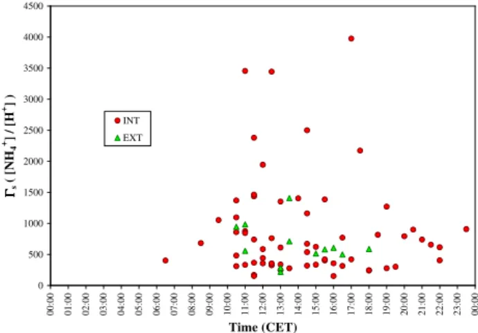
3.3 Micrometeorological estimates ofŴs

The analysis of flux reversal occurrences (deposition to emis-sion or vice-versa) in dry and mostly daytime conditions yields estimates ofŴs (Eq. 12) for the INT field in the range

150–4000 (Fig. 5), with a median of 620 and an arithmetic mean value of 875 (N=64). Values were not significantly different for measurements made in the EXT field in 2006, with a range of 220–1400, a median of 585 and an average of 659 (N=12). These estimates were obtained from flux data selected using a surface relative humidity threshold of 81% to distinguish “dry” from “wet” conditions, as this cor-responds to the deliquescence point of ammonium sulphate salts present on leaf cuticles (Flechard et al., 1999).

Given the necessary data selection process (dry, back-ground conditions only), there were very few or noŴs

esti-mates for night-time, early morning, autumn, winter, as well as during the days following fertilisation, so that diurnal and seasonal variations were difficult to assess. As the grass was wet most mornings due to dewfall, most estimates ofŴswere

obtained from 10:00 CET onwards (Fig. 5), after evaporation of leaf surface water films. No systematic diurnal cycle in

Ŵs can be detected in Fig. 5, although mostŴs values above

1000 were measured in the interval 10:30–18:00 CET. There were no clear seasonal patterns or event-related influences (cuts, fertilisation). Further, very few estimates ofŴs were

obtained in 2006 as the exchange in the INT field was then dominated by deposition (Fig. 1) with therefore very few flux sign reversals.

3.4 Annual NH3budget

An observation-based annual NH3budget was calculated for the INT field following the gap-filling procedure as described in Sect. 2.4 and in Spirig et al. (2010). As there were no clear differences, between the EXT and INT fields during back-ground phases, in flux patterns (Fig. 1) and stomatal com-pensation points (Fig. 5), and since fluxes could only be

mea-0 500 1000 1500 2000 2500 3000 3500 4000 4500

0

0

:0

0

0

1

:0

0

0

2

:0

0

0

3

:0

0

0

4

:0

0

0

5

:0

0

0

6

:0

0

0

7

:0

0

0

8

:0

0

0

9

:0

0

1

0

:0

0

1

1

:0

0

1

2

:0

0

1

3

:0

0

1

4

:0

0

1

5

:0

0

1

6

:0

0

1

7

:0

0

1

8

:0

0

1

9

:0

0

2

0

:0

0

2

1

:0

0

2

2

:0

0

2

3

:0

0

0

0

:0

0

Time (CET)

ΓΓΓΓs

(

[

N

H4

+]

/

[H

+]

)

INT EXT

Fig. 5. Apoplastic Ŵs ratio estimated from micrometeorological

flux measurements (Eqs. 6 and 12), shown as a function of time of day.

sured on one of the two fields at a time, the two datasets were merged to calculate the cumulative background component of the INT budget. ModeledRw was calculated according

to Eq. (14), andχs was computed on the basis of Eq. (12)

using the medianŴs values of 620 and 585 for the INT and

EXT fields, respectively, for the whole monitoring period. For slurry-induced emission events, gap-filling was achieved by using an interpolation ofŴcanopy for the first few hours and days following manure application (Spirig et al., 2010).

The NH3 budget for the period July 2006 through Oc-tober 2007 was +27.2 kg N ha−1, with a cumulative gross NH3 emission by 6 slurry applications of +30.4 kg N ha−1 and a net uptake of−3.2 kg N ha−1in background exchange (Fig. 6). For the one-year interval 1 July 2006 to 30 June 2007, which included only four slurry events, and during which flux data capture was better, the net budget was

+17.0 kg N ha−1yr−1 with slurry-induced NH3 emissions of +20.0 kg N ha−1yr−1 and background dry deposition of

−3.0 kg N ha−1yr−1.

C. R. Flechard et al.: The ammonia budget of fertilised grassland 547 -4 0 4 8 12 16 20 24 28 32 Ju l. 0 6 A u g .0 6 S ep .0 6 O ct .0 6 N o v .0 6 D ec .0 6 Ja n .0 7 F eb .0 7 M ar .0 7 A p r. 0 7 M ay .0 7 Ju n .0 7 Ju l. 0 7 A u g .0 7 S ep .0 7 O ct .0 7 N o v .0 7 C u m u la ti v e N H3 f lu x ( k g N h a -1)

Background (measured) Background (model gap-filled) Slurry events Total net exchange

Emission

Deposition

Fig. 6. Cumulative 17-month NH3 exchange with contributions

from background exchange and slurry application events.

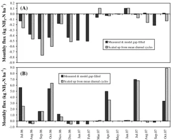
period mostly focused on the first few days following the application of slurry and thus background fluxes were under-represented in the monthly dataset; this statistical bias meant that the diurnal cycle approach over-estimated the monthly flux by a factor of 2.6. This demonstrates the importance of careful, process-based, gap-filling procedures for the calcu-lation of annual budgets, for both background exchange and peak emission events.

4 Discussion

4.1 Compensation point modeling of NH3exchange 4.1.1 Ammonia emission potential: apoplast vs. other

canopy sources

There have been numerous measurements and micromete-orological estimates of the apoplasticŴs ratio in European

grasslands over the last 10 yr, yet a current challenge in the NH3 emission/deposition modeling community remains to understand and predict temporal and spatial variations inŴs

for application in regional-scale atmospheric models. Total foliar N and NH+₄ content and the stomatal compensation point have been shown to increase with either elevated atmo-spheric deposition in semi-natural systems, or with fertilisa-tion level in agricultural environments (Pitcairn et al., 1998; Mattsson and Schjoerring, 2002; Herrmann et al., 2001), so that measurements ofŴs at any one site cannot be applied to

all grasslands across the countryside. Ecosystem modeling may ultimately provide a sound basis for predicting stomatal compensation points not only for grasslands (Riedo et al., 2002) but also for a wider range of ecosystems, and valida-tion measurements are needed.

By contrast to the direct measurement of NH+₄ and H+ concentrations after extraction of the apoplastic fluid (e.g. Mattsson et al., 2009), we present micrometeorological es-timates of Ŵs based on the assumption that under selected

dry conditions, most of the exchange takes place between stomata and the atmosphere (Sect. 2.3.3). The definition of a “dry” surface is thus a critical step in deriving Ŵs.

Fig--1.0 0.0 1.0 2.0 3.0 4.0 5.0 6.0 7.0 8.0 9.0 Ju l. 0 6 A u g .0 6 S ep .0 6 O c t. 0 6 N o v .0 6 D ec .0 6 Ja n .0 7 F eb .0 7 M a r. 0 7 A p r. 0 7 M ay .0 7 Ju n .0 7 Ju l. 0 7 A u g .0 7 S ep .0 7 O c t. 0 7 M on th ly f lu x ( k g N H3 -N h a -1)

Measured & model gap-filled Scaled up from mean diurnal cycles

-0.9 -0.8 -0.7 -0.6 -0.5 -0.4 -0.3 -0.2 -0.1 0.0 0.1 0.2 M on th ly f lu x ( k g N H3 -N h a -1)

Measured & model gap-filled Scaled up from mean diurnal cycles

(B) (A)

Fig. 7. Effect of flux integration method on monthly NH3

bud-gets. (A)background exchange only;(B)total fluxes (background exchange and slurry events).

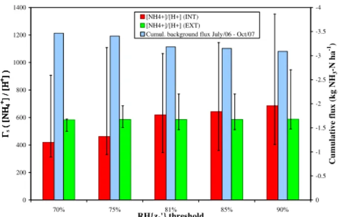
ure 8 presents the sensitivity of the meanŴs to the threshold

for RH{z′₀}used in selecting micrometeorological flux data, which by default is set to 81%. For the INT data, the median

Ŵsincreases from 420 at a threshold of 70%, to 620 at 81%,

to 686 at 90% (a slope of 14Ŵsunits for each additional 1%

in the threshold). This means that a greater stomatal source strength is required to overcome an increasing leaf surface sink capacity as relative humidity and the cuticular water film thickness both increase (Burkhardt et al., 2009). For the EXT field, no trend is visible as most data points were measured in very dry conditions at RH below 70%. The sensitivity of the cumulated background flux, which is based on measured flux data and gap-filled with theχs−Rwmodel, is very low, as the

overall net deposition flux increases by 9% for a threshold of 70%, and decreases by only 3% for a threshold of 90%, rela-tive to the base run with a threshold of 81% (Fig. 8).

The medianŴs value of 620 for the INT field at

Oensin-gen is rather at the low end of estimates for intensively man-aged grasslands found in the literature. Over a fertilised pas-ture at Zegveld in The Netherlands, Plantaz (1998) derived an apoplastic NH+₄ concentration of 775 µM, equivalent to

Ŵs=4900 with a pH of 6.8, for conditions outside

fertilisa-tion events. Estimates of apoplastic NH+₄ concentration ob-tained by Mosquera et al. (2001) at the Schagerbrug site in the Netherlands, using the apoplastic extraction technique, ranged over two orders of magnitude up to 6000 µM, equiva-lent toŴs=6000 with a pH of 6. Wichink Kruit et al. (2007)

derived an apoplastic Ŵs=2200 over grassland, which was

unfertilised but located in an area of intensive agriculture in the Southern Netherlands, where atmospheric N deposition is high. Over cut grassland at Burrington Moor in the UK, Sutton et al. (1997) estimated a value of Ŵs=1300 before

cutting, and a value ofŴs=10 000 after cutting. Similarly,

0 200 400 600 800 1000 1200 1400

70% 75% 81% 85% 90%

RH{z0'} threshold

ΓΓΓΓs

(

[ΝΗ

(

[ΝΗ

(

[ΝΗ

(

[ΝΗ

4444

++++] /

[Η

] /

[Η

] /

[Η

] /

[Η

++++] )] )] )] )

-4

-3.5

-3

-2.5

-2

-1.5

-1

-0.5

0

C

u

m

u

la

ti

v

e

f

lu

x

(

k

g

N

H3

-N

h

a

-1)

[NH4+]/[H+] (INT) [NH4+]/[H+] (EXT)

Cumul. background flux July/06 - Oct/07

Fig. 8.Sensitivity of the medianŴsestimate to the relative humidity

threshold used for the selection of “dry” surface conditions (verti-cal bars indicate 25th and 75th percentiles), and effect on the cu-mulative background exchange calculated using (model) gap-filled fluxes.

Milford (2004) estimated a “pre-cut” and winterŴs of 630,

an increasing “post-cut”Ŵs up to a “post-fertilisation”

(am-monium nitrate pellets) level of 28 000, and a “grazing”Ŵs

of 4000. The UK-CBED regional atmospheric deposition model (Smith et al., 2000) assumes a constantŴs value of

3800 for all managed and improved grasslands.

By comparison, over unfertilised, semi-natural grassland at Melpitz in Eastern Germany, Spindler et al. (2001) de-rive Ŵs in the range 150–1000. Over unimproved,

ex-tensive moorland at Auchencorth Moss in Southern Scot-land, Flechard et al. (1999) measured predominantly depo-sition fluxes, although there were also occasional emissions, which were a consequence of an apoplasticŴs ratio of 180.

Likewise, over semi-arid extensive grassland in Hungary, Horv´ath et al. (2005) found a backgroundŴsof around 100.

The contrast between published Ŵs values for fertilised

and unfertilised grasslands suggest a strong influence of added N on the foliar emission potential. It is logical to as-sume that some of the NH+₄ in slurry that percolates and is adsorbed to soil particles will eventually be taken up by roots, migrate upwards to the apoplast and participate in stomata-mediated exchange. However, the effect may not be as sig-nificant, nor as long-lasting, as may be expected on the basis of previous studies. New research demonstrates a rapid in-crease ofŴs in response to mineral fertiliser application, but

this is followed by an exponential decrease ofŴs over 10 d

back to pre-fertilisation levels (Mattsson et al., 2009; Loubet et al., 2002). Further, estimates ofŴs derived from

microm-eteorological flux measurements made above a canopy inte-grate the net effect of all component parts of the ecosystem. Thus thecanopycompensation pointχcis only a fair

reflec-tion of thestomatalcompensation pointχsif other emission

sources within the canopy, e.g. soil and litter, as well as de-position pathways, may be considered negligible at a given

point in time. It is increasingly recognised that some of the highest estimates of Ŵs (>5000–10 000) originally derived

in some studies were biased upwards by emission poten-tials in the leaf litter (Burkhardt et al., 2009), in urine and dung on the soil surface in grazed systems (Milford, 2004), or in the remains of fertiliser some time after its field appli-cation (Harper et al., 2000). By filtering out slurry events from background exchange, this study seeks to provide an unbiased estimate of the emission potential of grassland per se, which might therefore appear lower than previously be-lieved. TheŴs estimates at Oensingen (Fig. 5) are

nonethe-less thoroughly compatible with the range of values 200– 2000 measured using the vacuum infiltration technique by van Hove et al. (2002) inLolium perenneL. at Wageningen in the Netherlands, and with the mean value of 305 by Matts-son et al. (2009), and a range of 100–600 (PerMatts-sonne et al., 2009), at Braunschweig in Germany. The OensingenŴs

esti-mates are substantially higher than at another cut grassland in Switzerland at Kerzersmoos (Herrmann et al., 2001), where

Ŵs ranged from 50 to 100; the lower mineral fertilisation

rates of 80 to 160 kg N ha−1yr−1(vs. >200 kg N ha−1yr−1 at Oensingen) may be responsible in part for the difference.

Contrary to expectation no significant difference in Ŵs

could be detected between the INT and EXT treatments at Oensingen. However, the experiment was not designed with this objective in mind, with NH3fluxes being measured on the INT field most of the time and on the EXT field on only two occasions in July (1 week) and September 2006 (2.5 weeks). Indeed, most estimates ofŴs for the EXT field

were obtained in September 2006, a few days after the EXT field had been cut (Fig. 1), and thusŴsderived from

microm-eteorological fluxes may not have reflected the sole foliar emission potential, but also a contribution by the leaf litter following the removal of grass (Milford, 2004; Burkhardt et al., 2009).

Light diurnal fluctuations inŴs have been demonstrated

in grassland using the apoplast vaccuum infiltration tech-nique (Herrmann et al., 2009), with highest values occur-ring around noon, although diurnal changes were overshad-owed by day-to-day dynamics related to management (cut, fertilisation). The stomatal compensation point model of Wu et al. (2009) predicts a strongŴs peak in mid-afternoon

and a night-time/early morning minimum, which are mostly driven by pH changes. At Oensingen, the analysis of diur-nal variations in Ŵs (Fig. 5) was inconclusive, in part

be-cause the micrometeorological data selection procedure (dry conditions only; stomata open; change in flux direction) re-sults in fewŴs estimates being available overall and

espe-cially for night-time. Also, potential seasonal variations in

Ŵs (van Hove et al., 2002) make the interpretation of Fig. 5

rather difficult, as data for all seasons are pooled together. An alternative analysis (data not shown), where the diur-nal variations of the (dimensionless) ratio ofŴs to the daily,

weekly or monthly meanŴs were investigated, did not

C. R. Flechard et al.: The ammonia budget of fertilised grassland 549 Fig. 5, with daytime maximum of up to 2000–4000, and late

morning or early evening values below 500, is likely a re-flection of seasonal variations rather than of diurnal changes. Seasonal dynamics themselves were difficult to assess, be-cause micrometeorologically derivedŴs data were unevenly

distributed through the year, with few estimates during the wetter months.

4.1.2 Vertical distribution of sources and sinks in the canopy

Recent advances in NH3exchange modeling have sought to quantify the contributions of the soil, leaf litter, fertiliser or manure, and grazing animal excreta, as well as the stomatal emission potential of grassland (Riedo et al., 2002; Personne et al., 2009) and other agricultural crops, such as oilseed rape (Nemitz et al., 2000, 2001), wheat (Nemitz et al., 2001) and soybean (Wu et al., 2009; Walker et al., 2006). Such mod-els recognise that, even in relatively short (<1 m), but rather closed canopies, turbulent transfer rates within the canopy need to be quantified in order to link up different layers dis-tributed vertically in the system, which all contribute to the net canopy/atmosphere exchange flux as measured by mi-crometeorology. Thus NH3 emissions by sources in soil or in the leaf litter at the soil surface, and by open stomata, may be partly recaptured by wet foliage. Personne et al. (2009) also argue that failing to account for the vertical tempera-ture gradient within a canopy induces errors in the compen-sation point, since the relationship ofχs to temperature is

exponential, and they thus recommend the coupling of en-ergy, water vapour and NH3exchange modules. Double- or multiple-layer models are useful tools to further process un-derstanding, but the increase in complexity, in the number of parameters needing to be fitted to measurements, and the temporal and spatial variations in source strength of the dif-ferent layers, have so far hindered their implementation in regional-scale atmospheric models.

In this paper the bi-directional exchange of NH3was mod-elled using a single-layer (χs−Rw) model for conditions

out-side slurry applications. A two-layer model was not applied due to the lack of detailed investigations of the soil, leaf litter and apoplastic emission potentials, i.e.Ŵ values measured by extraction, which would be required to simulate fluxes within the canopy (Personne et al., 2009; Mattsson et al., 2009; Burkhardt et al., 2009; Nemitz et al., 2001; Mannheim et al., 1997). Inferences from micrometeorological measure-ments made above the canopy, as in the present case, could only deliver bulk canopy potentials (Ŵs) and resistances (Rs,

Rw), which are consistent with, and directly applicable in,

single-layer models. No straightforward interpretations of the same data could be made in relation to the distribution of sources and sinks in different layers, even though a detailed mechanistic understanding of all exchange processes is sci-entifically desirable (Nemitz et al., 2001).

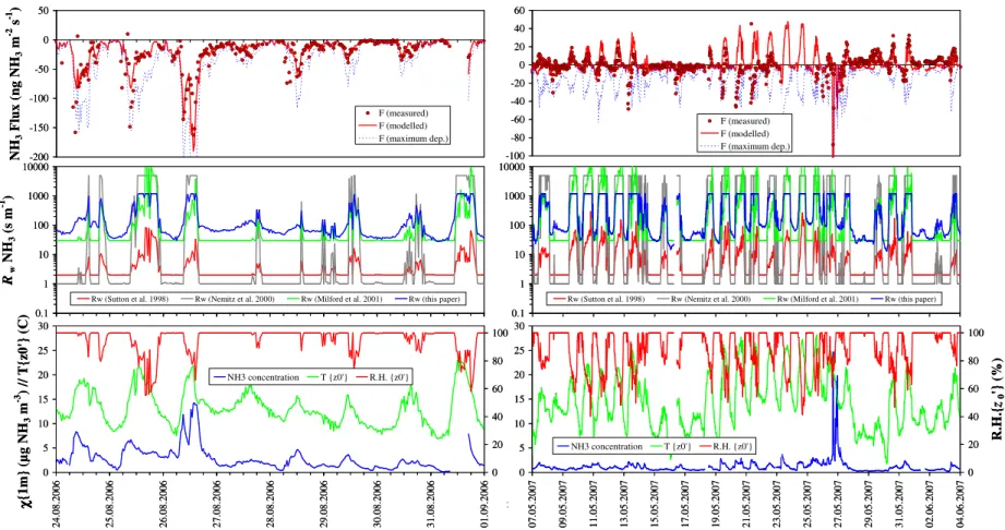
Model performance was best when the canopy was short (<20 cm) and rather sparse, such as during the summer of 2006 (Fig. 9, left), and when the exchange was deposition-dominated. In spring 2007 (Fig. 9, right), however, the canopy was taller (up to 35 cm) and thicker, and the flux was clearly bi-directional. During the first 10 d (7–17 May 2007) and the last week (27 May–4 June 2007) of the time series shown, the single-layer model performs rather well, simulating the measured day-time emission and night-time uptake, but the agreement is less favourable in the interval 18–26 May 2007. Here, average ambient temperature was higher, leading to higher modelled emissions, which were not systematically confirmed by the measurements. Figure 9 (bottom frames) also shows the markedly different patterns in atmospheric NH3concentrations between 2006 and 2007, with the generally higher ambient levels in 2006 leading to frequent deposition, and the lower levels in 2007 trigger-ing more emissions. Overall, model performance was rather good as the grass canopy was generally very short (70% of the time<15 cm; 81% of the time<20 cm; 86% of the time

<25 cm, between 1 July 2006 and 31 October 2007). The observed reduction over time in the NH3 source strength after slurry application (Fig. 2b, c) is a consequence of the NH+₄ pool decreasing due to both NH3 volatilisation and absorption by the soil. As the application of manure systematically occurred shortly after grass cuts, the canopy was always very short (<10 cm) and open during the first few days of slurry emission events. Thus the canopy may be treated as a single-layer for the purpose of gap-filling, with the proposed procedure (Spirig et al., 2010) based on a semi-empirical, semi-mechanistic approach involving the interpo-latedŴslurryratio.

4.1.3 Non-stomatal NH3sink

The parameterisation ofRw proposed in Eq. (14) and Fig. 4

corroborates the well-documented influence of leaf wetness via a surrogate in relative humidity (Sutton et al., 1998; Smith et al., 2000; Simpson et al., 2003) or in vapour pres-sure deficit (vpd) (Nemitz et al., 2000). Other models also use an RH-dependent non-stomatal resistance for water sol-uble trace gases like SO2 (Erisman et al., 1994; Zhang et al., 2003). However, the temperature control ofRw has not

gained much attention, and is rarely included in parameter-isations (Smith et al., 2000; Simpson et al., 2003), except in the case of frozen surfaces, whereRw increases asT

de-creases below O◦C (Wesely, 1989; Erisman et al. 1994; Zhang et al., 2003). Above freezing, temperature exerts a major forcing on trace gas solubility (Henry’s law), dis-sociation in water, and heterogeneous reaction rates (Sein-feld and Pandis, 2006), which all control surface uptake rates (Flechard et al., 1999; Flechard and Fowler, 2008). The influ-ence of temperature has often been overshadowed by that of RH, as the two variables tend to be anti-correlated on a daily-and annual basis in Europe, but the Oensingen data do show

C. R. Flechard et al .: The ammonia b udget of fertilised -100 -80 -60 -40 -20 0 20 40 60 F (measured) F (modelled) F (maximum dep.)

0 5 10 15 20 25 30 0 7 .0 5 .2 0 0 7 0 9 .0 5 .2 0 0 7 1 1 .0 5 .2 0 0 7 1 3 .0 5 .2 0 0 7 1 5 .0 5 .2 0 0 7 1 7 .0 5 .2 0 0 7 1 9 .0 5 .2 0 0 7 2 1 .0 5 .2 0 0 7 2 3 .0 5 .2 0 0 7 2 5 .0 5 .2 0 0 7 2 7 .0 5 .2 0 0 7 2 9 .0 5 .2 0 0 7 3 1 .0 5 .2 0 0 7 0 2 .0 6 .2 0 0 7 0 4 .0 6 .2 0 0 7 χχχχ 3 0 20 40 60 80 100 R .H .{ z0 '} ( % )

NH3 concentration T {z0'} R.H. {z0'} 0.1 1 10 100 1000 10000

Rw (Sutton et al. 1998) Rw (Nemitz et al. 2000) Rw (Milford et al. 2001) Rw (this paper) -100 -80 -60 -40 -20 0 20 40 60 F (measured) F (modelled) F (maximum dep.)

0 5 10 15 20 25 30 0 7 .0 5 .2 0 0 7 0 9 .0 5 .2 0 0 7 1 1 .0 5 .2 0 0 7 1 3 .0 5 .2 0 0 7 1 5 .0 5 .2 0 0 7 1 7 .0 5 .2 0 0 7 1 9 .0 5 .2 0 0 7 2 1 .0 5 .2 0 0 7 2 3 .0 5 .2 0 0 7 2 5 .0 5 .2 0 0 7 2 7 .0 5 .2 0 0 7 2 9 .0 5 .2 0 0 7 3 1 .0 5 .2 0 0 7 0 2 .0 6 .2 0 0 7 0 4 .0 6 .2 0 0 7 χχχχ 3 0 20 40 60 80 100 R .H .{ z0 '} ( % )

NH3 concentration T {z0'} R.H. {z0'} 0.1 1 10 100 1000 10000

Rw (Sutton et al. 1998) Rw (Nemitz et al. 2000) Rw (Milford et al. 2001) Rw (this paper) -200 -150 -100 -50 0 50 N H3 F lu x ( n g N H3 m

-2 s -1 )

F (measured) F (modelled) F (maximum dep.)

0.1 1 10 100 1000 10000 Rw N H3 ( s m -1 )

Rw (Sutton et al. 1998) Rw (Nemitz et al. 2000) Rw (Milford et al. 2001) Rw (this paper)

0 5 10 15 20 25 30 2 4 .0 8 .2 0 0 6 2 5 .0 8 .2 0 0 6 2 6 .0 8 .2 0 0 6 2 7 .0 8 .2 0 0 6 2 8 .0 8 .2 0 0 6 2 9 .0 8 .2 0 0 6 3 0 .0 8 .2 0 0 6 3 1 .0 8 .2 0 0 6 0 1 .0 9 .2 0 0 6 χχχχ {1 m } (µ g N H3 m -3 ) // T {z 0 '} ( C ) 0 20 40 60 80 100

NH3 concentration T {z0'} R.H. {z0'} -200 -150 -100 -50 0 50 N H3 F lu x ( n g N H3 m

-2 s -1 )

F (measured) F (modelled) F (maximum dep.)

0.1 1 10 100 1000 10000 Rw N H3 ( s m -1 )

Rw (Sutton et al. 1998) Rw (Nemitz et al. 2000) Rw (Milford et al. 2001) Rw (this paper)

0 5 10 15 20 25 30 2 4 .0 8 .2 0 0 6 2 5 .0 8 .2 0 0 6 2 6 .0 8 .2 0 0 6 2 7 .0 8 .2 0 0 6 2 8 .0 8 .2 0 0 6 2 9 .0 8 .2 0 0 6 3 0 .0 8 .2 0 0 6 3 1 .0 8 .2 0 0 6 0 1 .0 9 .2 0 0 6 χχχχ {1 m } (µ g N H3 m -3 ) // T {z 0 '} ( C ) 0 20 40 60 80 100

NH3 concentration T {z0'} R.H. {z0'}

Fig. 9.Measured and modeled background NH3flux, and concentration and meteorological/environmental drivers for contrasting conditions in summer 2006 (left) and in spring 2007

(right). The non-stomatal resistance (Rw) is compared with earlier parameterisations. The maximum deposition flux is calculated assuming that atmospheric turbulence is the only limit

to deposition andRcis zero (perfect sink). 7,