www.biogeosciences.net/10/2683/2013/ doi:10.5194/bg-10-2683-2013
© Author(s) 2013. CC Attribution 3.0 License.
Biogeosciences
Geoscientiic
Geoscientiic
Geoscientiic
Geoscientiic
Analysis of a 39-year continuous atmospheric CO
2
record from
Baring Head, New Zealand
B. B. Stephens1,2, G. W. Brailsford1, A. J. Gomez3, K. Riedel1, S. E. Mikaloff Fletcher1, S. Nichol1, and M. Manning3
1National Institute of Water and Atmospheric Research, Wellington, New Zealand 2National Center for Atmospheric Research, Boulder, Colorado, USA
3Victoria University, Wellington, New Zealand
Correspondence to:B. B. Stephens ([email protected])
Received: 15 September 2012 – Published in Biogeosciences Discuss.: 31 October 2012 Revised: 5 March 2013 – Accepted: 13 March 2013 – Published: 23 April 2013
Abstract.We present an analysis of a 39-year record of
con-tinuous atmospheric CO2observations made at Baring Head,
New Zealand, filtered for steady background CO2mole
frac-tions during southerly wind condifrac-tions. We discuss relation-ships between variability in the filtered CO2time series and
regional to global carbon cycling. Baring Head is well situ-ated to sample air that has been isolsitu-ated from terrestrial in-fluences over the Southern Ocean, and experiences extended episodes of strong southerly winds with low CO2
variabil-ity. The filtered Baring Head CO2 record reveals an
aver-age seasonal cycle with amplitude of 0.95 ppm that is 13 % smaller and 3 weeks earlier in phase than that at the South Pole. Seasonal variations in a given year are sensitive to the timing and magnitude of the combined influences of South-ern Ocean CO2fluxes and terrestrial fluxes from both
hemi-spheres. The amplitude of the seasonal cycle varies through-out the record, but we find no significant long-term seasonal changes with respect to the South Pole. Interannual varia-tions in CO2 growth rate in the Baring Head record closely
match the El Ni˜no-Southern Oscillation, reflecting the global reach of CO2 mole fraction anomalies associated with this
cycle. We use atmospheric transport model results to investi-gate contributions to seasonal and annual-mean components of the observed CO2record. Long-term trends in mean
gra-dients between Baring Head and other stations are predom-inately due to increases in Northern Hemisphere fossil-fuel burning and Southern Ocean CO2uptake, for which there
re-mains a wide range of future estimates. We find that the pos-tulated recent reduction in the efficiency of Southern Ocean
anthropogenic CO2 uptake, as a result of increased zonal
winds, is too small to be detectable as significant differences in atmospheric CO2 between mid to high latitude Southern
Hemisphere observing stations.
1 Introduction
The future trajectory of carbon exchange between the atmo-sphere and the earth’s oceans and terrestrial ecosystems re-mains a primary uncertainty in climate projections (IPCC, 2007). Predicting the response of global carbon fluxes to expected changes in atmospheric CO2, temperature,
precip-itation, and surface winds requires a better understanding of how and why these fluxes vary on synoptic to decadal timescales (Friedlingstein et al., 2006; Le Qu´er´e et al., 2007; Zickfeld et al., 2008), which in turn requires long-term, high-quality, and globally distributed observations of atmospheric CO2 mole fractions (Keeling, 1961; Keeling et al., 2001;
R¨odenbeck et al., 2003; Gurney et al., 2008; Patra et al., 2008).
As the primary area for the exchange of heat and gases be-tween recently upwelled surface waters and the atmosphere, the Southern Ocean is a region of critical importance for future climate change and atmospheric CO2 (Sarmiento et
mediated by varying influences associated with changes in solubility, biological, and anthropogenic forcing (Sarmiento et al., 1998; Caldeira and Duffy, 2000; Zickfeld et al., 2008; Lovenduski and Ito, 2009). Observations over the past several decades have suggested a significant poleward in-tensification and strengthening of Southern Ocean winds (Thompson and Solomon, 2002; Marshall, 2003), yet it is unclear what effect these changes are having on deep-water ventilation (Saenko et al., 2005; B¨oning et al., 2008) or what effect ventilation changes may be having on air-sea CO2
fluxes (Wetzel et al., 2005; Le Qu´er´e et al., 2007; Lovenduski et al., 2007; Law et al., 2008; Zickfeld et al., 2008; Lenton et al., 2009; Lovenduski and Ito, 2009; Takahashi et al., 2009). Long-term atmospheric CO2records at mid to high
south-ern latitudes have significant potential to shed light on past and ongoing changes in Southern Ocean CO2fluxes.
How-ever, the available records are few and regional background CO2 gradients induced by changes in the Southern Ocean
carbon sink are small, which makes their interpretation by atmospheric transport models challenging (Law et al., 2003; 2008). As a consequence, the available records are important and should be examined closely to improve their compatibil-ity across the global network and to maximize their scientific utility through data-based analyses.
One of the longest CO2records comes from Baring Head,
New Zealand (BHD), where continuous instruments have recorded measurements since 1972 (Lowe et al., 1979; Man-ning and Pohl, 1986; ManMan-ning et al., 1994; Brailsford et al., 2012) and are currently operated by staff of the New Zealand National Institute of Water and Atmospheric Re-search (NIWA). These data have been used in studies in-vestigating the global carbon cycle and in community data synthesis products (e.g., Keeling et al., 1989a; Keeling et al., 2001; Gurney et al., 2002; Le Qu´er´e et al., 2007; Globalview-CO2, 2011; WDCGG, 2012). There are relatively few
at-mospheric CO2observing sites in the Southern Hemisphere.
Other notable long-term sites include the South Pole (SPO), with flasks collected by Scripps Institution of Oceanogra-phy (SIO) since 1957 and in situ measurements by the US National Oceanic and Atmospheric Administration (NOAA) since 1976, and Cape Grim, Tasmania, with in situ measure-ments by the Commonwealth Scientific and Industrial Re-search Organisation also since 1976. Of the 17 active sites south of 30◦S, only 8 record in situ CO
2 measurements
(WDCGG, 2012). As a member of this small group, the Bar-ing Head record is particularly valuable for addressBar-ing ques-tions about interannual variability and trends for the carbon cycle at high southern latitudes and globally. Lowe et al. (1979) discussed the results from the first 4 yr of this dataset, describing the secular trend and seasonal cycle. Here, we present a newly reprocessed version of the full dataset and its variability with respect to other stations and important cli-mate processes. A companion paper details the history of the site, measurement techniques, calibration methodology, and intercomparison results (Brailsford et al., 2012).
To aid interpretation of the Baring Head CO2time series
and provide clues to sources of the observed trends and vari-ability, we include measurements from the SIO CO2program
made on flasks collected at the South Pole and by in situ in-strumentation at Mauna Loa Observatory in Hawaii (MLO) (Keeling et al., 2001). The high time resolution of the Bar-ing Head data allows for robust identification of background mole fractions as well as analyses of synoptic scale pro-cesses. In this paper, we focus on the interpretation of mea-surements that have been filtered to sample during steady CO2 conditions when air is arriving from the high-latitude
Southern Ocean. Aspects of the regional information con-tained in short-term variations will be the focus of subse-quent research. In Sect. 2 we summarize the Baring Head site characteristics including information on the origins of air masses arriving at the site, the selection criteria for steady periods, and our atmospheric transport modeling methods. In Sect. 3, we analyze and discuss annual mean mole fractions, seasonal and interannual variations, and long-term trends in the CO2time series and their relationship to Southern Ocean
and global carbon exchanges.
2 Background and methods
2.1 Site location and air origins
In 1970, in conjunction with the Department of Scientific and Industrial Research (DSIR, predecessor to NIWA) in New Zealand, C.D. Keeling’s group from SIO established a non-dispersive infrared (NDIR) analyzer at Makara (41.2473 S, 174.6944 E) about 15 km northwest of Wellington and 1 km inland from the west coast of the North Island, New Zealand (Fig. 1a). However, the first 1.5 yr of measurements at this site suggested that it was too strongly influenced by local ter-restrial signals, and the analyzer was moved to Baring Head (41.4083 S, 174.8710◦E) in December, 1972. The measure-ments of atmospheric CO2at the Baring Head site have
con-tinued to the present, making it the longest running in situ atmospheric CO2 observing station in the Southern
Hemi-sphere and the second longest globally.
Fig. 1.Maps showing(a)the location of Baring Head (BHD) and other landmarks, and(b)clustered results of 20 yr (1988–2007) of twice-daily 4-day back-trajectory calculations, with percentages in-dicated for each cluster. In(a), labels also indicate Makara (MAK) and Wellington (WLG) on the North Island, and colors indicate forests (green), inland water (blue), populated areas (dark gray), non-forested land (beige), and above tree line (light gray). In(b), color shading indicates a logarithm of the percentage of trajectories crossing a given latitude/longitude square. The+symbol indicates the location of TM3 model output used for comparison to steady pe-riod data in order to avoid local terrestrial influences in the model.
Baring Head was chosen to make CO2measurements
rep-resentative of large relatively homogeneous Southern Ocean air masses. Wind speeds at the site are typically high, reduc-ing the impacts of local sources. Also, southerly air arriv-ing at this site has often been out of contact with terrestrial sources and sinks of CO2for thousands of km, having
trav-elled over the Southern Ocean between the latitudes of 45 and 70◦S for the preceding week or more. These character-istics provide ideal conditions for determining background levels of atmospheric CO2 at these latitudes, but at other
times the site receives air that has recently passed over New
Zealand or Australia. Fig. 1b shows the results of a cluster-ing analysis on 20 yr of 4-day back trajectories for air ar-riving at Baring Head. The back trajectories were calculated every 12 h using the method of Gordon (1986) driven by winds from the New Zealand Meteorological Service prim-itive equation model. The clustering was performed using a convergentk-means procedure, which is described in Kidson (1994).
Onshore winds are usually associated with a repeating syn-optic pattern in which an anticyclone moves from the Tasman Sea, to the west of New Zealand, onto the country modu-lating the background westerly winds (Kidson, 2000). The Southern Alps of the South Island of New Zealand, which reach a height of 3750 m, have a major effect on air flow throughout the region. When the center of an anticyclone is well to the west of New Zealand, the mountain range acts to deflect air flow northward along the west coast of the South Island and then through the Cook Strait separating the North Island and the South Island. This results in a northwest wind in the strait that is further channeled by topography to a local wind at Baring Head that is from the north. Most of the back trajectories from the northwest sector in Fig. 1b correspond to local winds from the due north at Baring Head, although the model used to produce the back-trajectories does not have sufficient resolution to capture this topographic forc-ing. As the anticyclone moves eastward, a transition occurs to a regime in which air flows around the south of the South Island, and the local wind at Baring Head is from the south. This synoptic pattern is typically associated with a descend-ing air mass and back trajectories that come from around 55◦S and have not crossed land in at least 4 days. As the clustering analysis in Fig. 1b indicates, south and southeast arriving trajectories occur approximately 27 % of the time. Southerly wind events can persist for several days at a time and occur roughly 4 times per month in winter and 2 times per month in summer.
2.2 Data filtering
Isolating clean marine background measurements from those influenced by local terrestrial fluxes requires a data filter-ing scheme informed by a good knowledge of the local site and wind conditions and their influence on CO2
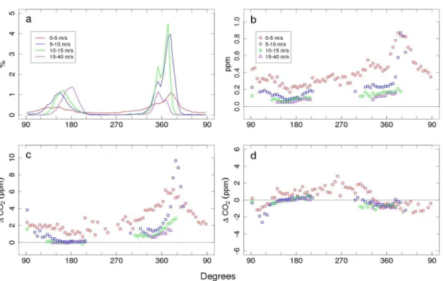
variabil-ity. As discussed above, the topography of the South Island, Cook Strait, and the mountains near Baring Head result in the site almost exclusively experiencing due northerly or due southerly winds that are often quite strong. Figure 2a shows frequency distributions for winds of different directions and speed. As this Fig. indicates, approximately 2/3 of the time the hourly average wind direction is within 30 degrees of north, and 1/2 of these winds are over 10 m s−1. The
remain-ing 1/3 of the time, the wind is primarily from the south, with 2/3 of these winds over 10 m s−1and the stronger winds
Fig. 2.Influence of wind speed and direction on CO2mole fractions and variability as derived from Baring Head data from 1997–2011. (a)Wind direction distributions for four different wind speed ranges shown as percentage of all winds in 5-degree increments.(b)Hourly CO2variability (1-sigma) as a function of wind direction for four different wind speed ranges.(c)Differences between nighttime (22:00– 04:00 LST) hourly mean observed CO2mole fractions and interpolated steady period data for four different wind speed ranges.(d)Same as (c)but for daytime (10:00–16:00 LST). For(b–d), points are only plotted if that wind direction and speed bin represents 0.05 % or greater of all wind conditions.
These wind conditions have a major influence on CO2
variability, with hourly standard deviations less than 0.2 ppm corresponding to strong northerlies and moderate and strong southerlies, and higher variability to weak winds and mod-erate northerlies (Fig. 2b). Although strong northerlies are often associated with low CO2variability, it is apparent from
comparing mole fractions measured during these episodes to those during southerlies that they still reflect significant ter-restrial influences. Figures 2c and d show that these strong northerlies are typically 1.0–1.5 ppm higher in CO2 during
night, and 0.5–1.0 ppm lower during day as a result of up-wind respiration and photosynthesis on the North Island. High daytime CO2 mole fractions during infrequent weak
westerlies likely result from emissions associated with the large populations in the city of Wellington and surrounding suburbs.
In order to obtain a baseline record representative of large marine air masses, we have employed a filter focused on re-trieving long durations of steady CO2mole fractions when
air arrived from the south without first crossing over the South Island (see Fig. 1). We start with a multi-step filter in which first “steady intervals” for either of two inlet lines are defined as intervals for which the CO2mole fraction has
a maximum standard deviation of 0.1 ppm for a minimum
length of 6 h. Then, overlapping steady intervals for one or both inlet lines are aggregated into “steady periods”, which can themselves have slowly trending mole fractions. Next, these steady periods are further screened to exclude cases when the wind was not from the south, and finally they are also screened to exclude cases when it is likely the air passed over the South Island before arriving at Baring Head. This last step is accomplished by requiring that the atmospheric pressure difference across the Southern Alps, as measured by the difference between pressure at Christchurch on the east coast and that at Hokitika on the west coast (Fig. 1a), be 1 mbar or greater averaged over the steady period (Manning and Pohl, 1986). We use the term “steady interval” to refer to a 6-plus hour span from a single inlet with 0.1 ppm or less standard deviation, and the term “steady period” to refer to a complete set of overlapping intervals, to be consistent with prior Baring Head data reports. Steady periods further fil-tered on meteorological conditions then represent what other investigators often call “background” or “baseline” data.
Fig. 3.Baring Head CO2time series, showing all hourly averages (black) and data filtered for steady southerly periods as described in the text (red). The filtered data are shown as average values for the entire steady period. The years from 1987–1994 with truncated hourly CO2peaks resulted from an intentional adjustment of the an-alyzer output range to increase sensitivity during southerly wind pe-riods, but sacrificing measurements during locally influenced high CO2episodes. With the focus on the steady period data, the hourly average record was not historically scrutinized. Low CO2anomalies in the hourly average record prior to 2002 likely result from instru-mentation problems, and work is currently underway to use hand-written notes to identify and filter such events out. Prior to 1978, high-rate measurements were recorded on strip charts, but only the steady period data are available in digital form. The plotted data prior to December 1972 are from the Makara site.
periods have been found to occur on average 36 times per year, last on average 17 h, and constitute 13 % of the com-plete observational record. This is significantly less than the percentage of southerly conditions because of the require-ment for the conditions to persist for 6 h. There is signifi-cant seasonal variability in the occurrence of steady periods and also some in their duration, with 67 % more periods, to-taling twice as much overall time, occurring in the winter months of June–August compared to the summer months of December–February. The southerly criterion excludes 13 % of steady CO2 periods, but less than 8 % in terms of time
as the northerly steady CO2periods tend to be shorter. The
Christchurch–Hokitika pressure difference excludes another 26 % of the remaining steady periods and 18 % in terms of time. Each of the resulting filtered steady periods is treated as a unique single event, and CO2 data reported to
com-munity data collections (Globalview-CO2, 2011; WDCGG,
2012) have historically consisted of average mole fractions, standard deviations, start times, and durations for each steady period. Figure 3 shows both the unfiltered and filtered CO2
time series for Baring Head. The smoothness of the steady period curve relative to the scatter of all hourly averages re-veals the power of this filtering method to isolate remote ma-rine signals. Simple filters based on hourly wind direction or within hour CO2variability are much less selective. The
fre-quency of steady periods found has varied from year to year.
Fig. 4.Results of STL decomposition of the Baring Head steady pe-riod CO2record.(a)trend component found using 10-year window, (b)interannual component found using 2-year window,(c)seasonal component using a 5-year window on monthly trends, and(d) re-mainder component. For(b–d), the y-axis scales are similar. The fits include data prior to December 1972 from the Makara site.
Although this may be the result of changes in atmospheric transport patterns or variable CO2 fluxes, variations in the
number of steady periods could also be related to changes in instrument procedures or performance (Brailsford et al., 2012).
We employ the detailed filter criteria to enable time-series analysis on low-variability background marine air and to in-vestigate questions about changes in Southern Ocean fluxes. Coarse-resolution models that use these filtered steady pe-riod Baring Head data or synthesized products based on them (Globalview-CO2, 2011) must account for this filtering to
ad-equately represent the observing conditions. Recognizing the ability of more recent models to combine higher resolution data with information on corresponding synoptic transport in order to infer fluxes on regional scales, we also make the hourly mean unfiltered CO2 time series publicly available,
along with values for short-term variability and winds.
2.3 Atmospheric transport modeling
To aid in interpreting the observations at Baring Head, we have used simulations from the fine grid version of the Trans-port Model version 3 (TM3) (Heimann and K¨orner, 2003), which has a resolution of ∼3.8◦ latitude by 5◦ longitude with 19 vertical levels. TM3 is a three-dimensional Eule-rian model driven by off-line winds from the NCEP reanal-ysis (Kalnay et al., 1996). TM3 has been included in sev-eral model intercomparison studies (e.g., Gurney et al., 2002; Gurney et al., 2003; Baker et al., 2006).
We used the CO2 sources and sinks from the
Fig. 5.Long-term average Baring Head and South Pole seasonal CO2cycles shown as monthly means of the STL fit seasonal com-ponent (symbols) along with 2-harmonic fits to detrended monthly mean data (lines). 18 months are shown with Jan–Jun repeated for clarity.
be able to isolate the influence of different regions and source processes on the station, CO2 from fossil-fuel emissions,
biomass burning, the terrestrial biosphere, and the oceans were each treated as separate tracers in the model and sepa-rated geographically according to the TransCom flux regions (Gurney et al., 2003). To determine the modeled sensitivity at a particular station to a particular source, we divide the corre-sponding CO2signal, averaged over the years 2003–2009, by
the corresponding source strength. The resulting sensitivities are similar to those found with other atmospheric transport models (Gurney et al., 2003). For our calculations, we ex-tract CO2values at a point 1000 km to the southwest of
Bar-ing Head (50◦S, 170◦E; see Fig. 1) to represent the filtered steady period Baring Head record, as the modeled values for Baring Head used no filtering for steady-CO2southerly wind
conditions. The selection of this point is somewhat arbitrary, but avoids local terrestrial influences and is close to the two southerly back-trajectory clusters (Fig. 1b).
3 Results and discussion
3.1 Time series
Salient features of the long-term filtered steady period record include (1) a long-term growth rate of approxi-mately 1.5 ppm yr−1driven by global fossil-fuel
consump-tion and deforestaconsump-tion, (2) annual-mean differences with re-spect to other stations consistent with fossil-fuel burning in the Northern Hemisphere and oceanic CO2 uptake in the
Southern Hemisphere, (3) a seasonal cycle of around 1 ppm amplitude related to ocean exchange in the Southern Hemi-sphere and the influence of terrestrial fluxes in both the Northern Hemisphere and Southern Hemisphere, (4) interan-nual variations in the long-term growth rate reflecting global and Southern Ocean carbon cycle processes, and (5)
long-term trends in differences from other stations, which have the potential to constrain trends in Southern Ocean CO2fluxes.
To visually decompose the variations on different time scales, we use the seasonal time-series decomposition by Loess (STL) routine (Cleveland and McRae, 1989; Cleve-land et al., 1990), which allows for changes in seasonal pat-terns over time. This routine fits locally weighted polynomial regressions to time series composed of all values from indi-vidual months, for example all average January values for the entire record, as well as the remaining deseasonalized trend, in an iterative process. The degrees to which the seasonal cy-cle and long-term trend are allowed to vary to fit the data are set by specifying the window for the seasonal and trend Loess fits. We use a seasonal cycle window of 5 yr and first run the procedure using a trend window of 121 months in-tended to reflect changes on decadal timescales. Then, after removing this component we run the procedure again with a trend window of 25 months to capture subdecadal compo-nents. Figure 4 shows the results of this STL calculation for Baring Head. We have run the same routine and parameters on South Pole flask and Mauna Loa continuous data from SIO for the overlapping years.
3.2 Annual-mean mole fractions
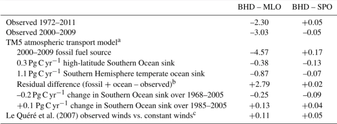
As shown in Table 1, the average difference over the entire 39-year record between Baring Head and Mauna Loa (BHD– MLO) is –2.30 ppm, and between Baring Head and the South Pole (BHD–SPO) is+0.05 ppm. For the decade 2000–2009, the average BHD–MLO difference is –3.03 ppm and the av-erage BHD–SPO difference is –0.05 ppm, opposite in sign to that for the full record. The Baring Head record exhibits in-creasingly lower mole fractions than the Mauna Loa record because of the predominance and growth of fossil-fuel CO2
emissions in the Northern Hemisphere and oceanic CO2
up-take in the Southern Hemisphere. Despite being further north than the South Pole, Baring Head shows similar and trend-ing lower annual-mean CO2mole fractions. This reflects the
greater influence of the increasing Southern Ocean CO2sink
on air at Baring Head (Keeling et al., 1989b, Kawa et al., 2004).
The TM3 model sensitivities (Sect. 2.3) scaled by 2000– 2009 fossil fuel CO2sources (Boden et al., 2009, as
extrap-olated by CarbonTracker 2010) result in an average BHD– MLO difference of –4.57 ppm and an average BHD–SPO difference of 0.17 ppm (Table 1). The TM3 model sensi-tivities suggests that a postulated 0.3 Pg C yr−1 sink in the
high-latitude Southern Ocean (Gruber et al., 2009) results in a –0.38 ppm BHD–MLO difference and a –0.13 ppm BHD–SPO difference. Furthermore, the model sensitivities predict that a plausible 1.1 Pg C yr−1 sink in the
Table 1.Observed and modeled intersite CO2differences (ppm).
BHD – MLO BHD – SPO
Observed 1972–2011 –2.30 +0.05
Observed 2000–2009 –3.03 –0.05
TM5 atmospheric transport modela
2000–2009 fossil fuel source –4.57 +0.17
0.3 Pg C yr−1high-latitude Southern Ocean sink –0.38 –0.13 1.1 Pg C yr−1Southern Hemisphere temperate ocean sink –0.87 –0.07 Residual difference (fossil+ocean – observed)b +2.79 +0.02 –0.2 Pg C yr−1change in Southern Ocean sink over 1968–2005 –0.25 –0.09
+0.1 Pg C yr−1change in Southern Ocean sink over 1985–2005 +0.13 +0.04 Le Qu´er´e et al. (2007) observed winds vs. constant windsc +0.11 +0.05
aDifferences shown are for (50◦S, 170◦E) – MLO and (50◦S, 170◦E) – SPO to represent filtered steady southerly period selection
of BHD data, as described in the text.
bTo the extent that the two nominal ocean sinks are correct, this represents the combined influence of tropical and Northern
Hemisphere land and ocean CO2exchange.
cDifferences shown are for MQA – MLO and MQA – SPO to represent steady southerly period selection of BHD data, as described
in the text.
BHD–SPO differences, because atmospheric transport gen-erates phase differences, they can have a larger effect on monthly site differences. Tropical and Northern Hemisphere terrestrial biosphere and ocean fluxes are responsible for countering the influence of the fossil-fuel source and South-ern Ocean sink on the BHD–MLO gradient, to produce the observed value (Table 1), but their relative proportion is model-dependent and a topic of active research (Stephens et al., 2007). TM3 and other models suggest that tropical and northern fluxes have little influence on the BHD–SPO differ-ences. The counteraction of the fossil-fuel source and South-ern Ocean sinks described above can explain the observed 2000–2009 annual-mean BHD–SPO difference well within the limits of uncertainty (Table 1).
3.3 Seasonal cycles
Figure 5 shows the average seasonal cycles at Baring Head, for filtered steady period data, and at South Pole for the 39 yr of the Baring Head record. The amplitude of the average Bar-ing Head cycle is 0.95 ppm with a late-winter maximum in September, and an autumn minimum in March. This cycle is 13 % smaller and 3 weeks earlier in phase compared to that at the South Pole. Both cycles are small relative to those at Northern Hemisphere stations, but their timing and am-plitudes may represent important tests for our understanding of hemispheric CO2fluxes and interhemispheric atmospheric
transport (Dargaville et al., 2003; Baker et al., 2006). Early studies recognized that seasonal cycles in atmo-spheric CO2at high southern latitudes represented the
com-bined influences of Northern Hemisphere terrestrial fluxes delayed by interhemispheric transport and Southern Hemi-sphere terrestrial and oceanic fluxes (Pearman and Hyson, 1980; Heimann and Keeling, 1989) but lacked sophisticated estimates of these processes. More recent models of
atmo-spheric CO2at high southern latitudes incorporate improved
knowledge of flux distributions and better transport, but still show differences in relative seasonal contributions at high southern latitudes (Erickson et al., 1996; Heimann et al., 1998; Dargaville et al., 2002; Roy et al., 2003; Gurney et al., 2004; Nevison et al., 2008; Takahashi et al., 2009). However, the general picture for the Baring Head record has remained relatively consistent over time, in which the influence from Northern Hemisphere terrestrial fluxes is lagged by approx-imately 6 months and reduced such that it is comparable in phase and magnitude to that from Southern Hemisphere ter-restrial fluxes (Heimann and Keeling, 1989; Heimann et al., 1998).
Figure 6 shows model-estimated contributions to the sea-sonal CO2cycle from various sources for the simulated point
to the southwest of Baring Head. These curves were obtained by fitting the CarbonTracker/TM3 model output for the years 2003–2009 with 2-harmonic seasonal cycles. The Northern Hemisphere and Southern Hemisphere terrestrial influences both have peaks in late austral winter (August–September) and troughs in austral autumn (March–April). The South-ern Hemisphere ocean contribution has a peak in late aus-tral autumn (May) and trough in early ausaus-tral summer (De-cember), comparable in magnitude and leading by around 5 months the Northern Hemisphere and Southern Hemi-sphere terrestrial influences, and reflecting thermal forcing at lower latitudes rather than biological forcing at high latitudes (Heimann et al., 1998; Takahashi et al., 2009). The combi-nation of these out-of-phase influences leads to a modeled Baring Head peak in atmospheric CO2in austral winter
Fig. 6.Contributions to the seasonal CO2cycle at Baring Head as simulated by TM3 forced by CarbonTracker 2010 fluxes (Peters et al., 2007). 18 months are shown with Jan–Jun repeated for clar-ity. The northern (N), tropical (T), and southern (S) allocations are based on the TransCom regions (Gurney et al., 2003) with tropi-cal divisions at approximately 15◦N and 15◦S. Total contributions from biomass burning (BB) and fossil-fuel emissions (FF) are also shown. The observed cycle from Fig. 5 is plotted again here for comparison to the total model curve.
In the model, both the oceanic and terrestrial contributions to the atmospheric CO2seasonal cycle are advanced in phase
at Baring Head relative to the South Pole (not shown), which reflects the mixing time needed for signals to propagate from further north and explains the resulting phase difference be-tween these two stations. The modeled Southern Ocean con-tribution is larger in amplitude at Baring Head than at South Pole. In the real atmosphere, this may result in a greater can-cellation of the out-of-phase terrestrial contribution, poten-tially explaining why the observed overall amplitude is lower at Baring Head than at the South Pole. However, our model simulations produce greater seasonal amplitude at Baring Head than both observed and modeled for South Pole. This highlights the sensitivity of the seasonal cycle at Baring Head to subtle shifts in timing and magnitude of the contributing influences, and suggests that further work to characterize the influence of interhemispheric transport on seasonal CO2
cy-cles in the Southern Hemisphere would be useful.
Because the resulting seasonal cycle is a delicate balance between multiple processes, it varies considerably from year to year, and can be hard to detect in some years (Fig. 3). Fig. 7 shows the interannually varying 5-year-smoothed sea-sonal components from STL fits to both Baring Head and South Pole, as well as the peak-to-peak amplitudes of these components. The amplitudes show some similarities, and in particular both sites show an increase in amplitude over the last 3 yr of the records, indicating that seasonal CO2
varia-tions are often consistent over large areas of the high south-ern latitudes. However, there are notable exceptions such as the large increase in amplitude at Baring Head in the early 1990s that was less pronounced at the South Pole.
Fig. 7. (a)Seasonal CO2cycle components from STL decompo-sition of Baring Head and South Pole records. Fits used a 5-year smoothing window on Loess fits to individual monthly time series. The BHD line is the same as that shown in Fig. 4c.(b) Seasonal CO2cycle peak-to-peak amplitudes from curves in(a). The fits in-clude data prior to December 1972 from the Makara site.
Any long-term changes in seasonal amplitude or phase at Baring Head might provide clues to trends in seasonal ex-change processes. Because so much of the seasonal forc-ing at Barforc-ing Head comes from further to the north, these changes cannot be uniquely attributed to changes at high southern latitudes. However, by differencing the seasonal variations at Baring Head and South Pole, it might be pos-sible to isolate the influence of Southern Hemisphere ocean fluxes, as changes in northern fluxes or interhemispheric exchange times are likely to affect both stations similarly. Figure 8 shows differences between monthly means from the Baring Head filtered steady period record and South Pole. Also shown are linear trend lines fit to early summer (November–January) and early winter (April–June) months, when the modeled influence of Southern Ocean fluxes at Baring Head is maximized. Based on hypothesized changes in the upwelling-driven outgassing of CO2 in the Southern
Ocean (Le Qu´er´e et al., 2007), we might expect to see dif-ferent trends in the BHD–SPO gradient in difdif-ferent seasons. There are no apparent differences in the summer and win-ter trends shown in Fig. 8, suggesting that any changes in the seasonal aspects of Southern Ocean CO2change are too
small to be detected by this metric.
3.4 Interannual variations
The global carbon cycle and atmospheric CO2mole fractions
Fig. 8.Monthly mean CO2differences between Baring Head and South Pole. Months during the peak (April–June, green) and trough (November–January, purple) of the modeled influence from South-ern Ocean fluxes (Fig. 6) are highlighted and fit with trend lines. The points prior to December 1972 are from the Makara site.
on land, leading to decreased photosynthesis and increased respiration and fire activity, while a smaller ocean response in the opposite direction results from less outgassing of CO2
from upwelled waters in the tropical Pacific (Feely et al., 1999; Zeng et al., 2005). The net result for atmospheric CO2
mole fractions is a positive correlation between CO2growth
rate and ENSO, with CO2 growth rate lagging ENSO by
around 5 months. Terrestrial carbon exchange also responds on similar timescales to large-scale temperature fluctuations not directly related to ENSO (Keeling et al., 2001).
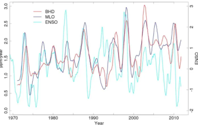
As Fig. 9 shows, the interannual fluctuations in CO2
growth rate at Baring Head are very similar to those at Mauna Loa, and both are closely related to the ENSO cycle. The high CO2 growth rates in the Baring Head record in 1973,
1979, 1983, 1987, 1998, 2002, and 2010 are all associated with leading El Ni˜no events. Although the upward response at BHD to one of the strongest El Ni˜nos in 1983 is less than at MLO, it is possible that other factors led to an increased growth rate at Baring Head the year prior to the El Ni˜no, ob-scuring the signal. The overall similarity to Mauna Loa high-lights the global reach of the atmospheric CO2variations in
response to ENSO. As estimated by correlation coefficients, ENSO can explain 23 % of the variability in the interannual component of the Mauna Loa STL fit at an optimal lag of 4 months, and can explain 16 % of the variability in the in-terannual component of the Baring Head STL fit at an opti-mal lag of 6 months. The peak in Mauna Loa growth rate in 1994–1995 is an example of warm global temperatures not associated with El Ni˜no (Keeling et al., 2001), though it is only partially matched by a Baring Head excursion in 1995.
Another important interannual forcing agent is the occur-rence of large volcanic eruptions, which have been shown to lead to global cooling and less respiration, as well as in-creased photosynthesis from more diffuse radiation as a re-sult of aerosol scattering (Gu et al., 2002; Reichenau and
Fig. 9.Baring Head and Mauna Loa CO2growth rate and the Mul-tivariate ENSO Index (Wolter and Timlin, 1993). The growth rates were calculated from the month-to-month change in the sum of the trend and interannual components of the STL fits to each record (Fig. 4a and b for BHD). All three time series have been smoothed with a 5-month running mean for clarity. The fits include data prior to December 1972 from the Makara site.
Esser, 2003; Mercado et al., 2009). These volcanic effects tend to mask or interrupt the otherwise tight connection to ENSO. For example, the extended weak El Ni˜no that started in 1991 did not lead to positive CO2 growth rate
anoma-lies because of the counteracting effects of the Mt. Pinatubo eruption in June 1991 (Gu et al., 2002; Reichenau and Esser, 2003).
Interannual differences between Baring Head and Mauna Loa could result from unique ENSO forcing at high southern latitudes, different mole fraction responses to tropical forcing in the Northern Hemisphere versus Southern Hemisphere, or unrelated phenomena. Previous studies (Le Qu´er´e et al., 2003; Verdy et al., 2007) have found evidence that the influ-ence of ENSO events can propagate into the Southern Ocean and lead to stronger westerlies, greater entrainment of deep water, and anomalous carbon outgassing. The extent to which ENSO influences the Southern Ocean varies, and this could explain some of the differences seen between Baring Head and Mauna Loa in Fig. 9. However, the 1986–1987 El Ni˜no had less influence on the Southern Ocean (Le Qu´er´e et al., 2003), while the Baring Head record appears to respond sim-ilarly to Mauna Loa in this event. An additional consideration in the case of Baring Head is that El Ni˜no influences on local wind patterns could affect the number or character of steady periods selected by the data filter (Mullan, 1996). However, we find no correlation between the number of steady periods and ENSO on monthly or yearly time scales..
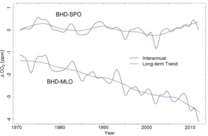
Fig. 10.BHD–SPO (top) and BHD–MLO (bottom) CO2differences in the interannual and trend components of the STL decomposition of the Baring Head, South Pole, and Mauna Loa records. The win-dow for the trend fits was 10 yr, and for the interannual fits was 2 yr. The fits include data prior to December 1972 from the Makara site.
CO2-rich water around Antarctica. Ocean biogeochemistry
models (Lenton and Matear, 2007; Lovenduski et al., 2007) and atmospheric inverse models (Butler et al., 2007) sug-gest anomalous Southern Ocean CO2outgassing of around
0.1 Pg C yr−1 per standard deviation of SAM. Butler et
al. (2007) were able to identify signals in atmospheric CO2
potentially associated with these flux changes by correlat-ing month-to-month tendencies in CO2 to the SAM index.
The correlations were greatest at Palmer Station Antarctica (PSA), and decreased further from the high-latitude South-ern Ocean. We have repeated the Butler et al. (2007) anal-ysis on our Baring Head data and found no significant cor-relation. This could either be because the postulated high-latitude Southern Ocean flux changes have a greater impact at PSA than they do at Baring Head, or, as discussed by But-ler et al. (2007), the correlation at PSA could result from local changes in wind direction that are different at Baring Head. The significant increase in seasonal amplitude (Fig. 7) then decrease in long-term growth rate (Fig. 3) from 1991– 1994 in the Baring Head record could be associated with the Mt. Pinatubo eruption as discussed above, but could also be related to a negative excursion in SAM that occurred from 1991–1993. Further research on possible mechanisms driv-ing these CO2changes is warranted.
Figure 10 shows the difference between the interannual and trend components of the Baring Head and Mauna Loa STL fits, and the difference between the interannual and trend components of the Baring Head and South Pole STL fits. Overall levels of interannual variability for high-latitude Southern Ocean carbon fluxes based on observational and modeling studies are on the order of ±0.15 Pg C yr−1 (1
sigma) (Louanchi and Hoppema, 2000; Le Qu´er´e et al., 2003; Butler et al., 2007; Lenton and Matear, 2007; Lovenduski et al., 2007). Based on our TM3 sensitivities, we would expect
this to appear in the BHD–MLO difference at the± 0.2 ppm level and the BHD–SPO difference at the± 0.05 ppm level. From Fig. 10, it is apparent that other processes such as lower latitude Southern Ocean fluxes, Northern Hemisphere processes combined with interhemispheric transport variabil-ity, or measurement or data-filtering biases must lead to the larger interannual variations of± 0.3 to 0.5 ppm. Similarities in the interannual BHD–MLO and BHD–SPO differences in-dicate times when the BHD record is most likely producing the variations.
3.5 Long-term trends
Despite the fact that year-to-year variations in Southern Ocean CO2fluxes have relatively small impacts on
year-to-year atmospheric CO2gradients, long-term trends in
South-ern Ocean carbon exchange can have major impacts on fu-ture global atmospheric CO2mole fractions. Because of the
large exchanges of heat and gases that occur between the at-mosphere and deep ocean waters at high southern latitudes, carbon fluxes in the Southern Ocean have long been recog-nized as a dominant factor in determining the ocean’s uptake of anthropogenic CO2 (Knox and McElroy, 1984;
Siegen-thaler and Wenk, 1984; and Sarmiento and Toggweiler, 1984; Sarmiento et al., 1998; Caldeira and Duffy, 2000). CO2
fluxes in this region are currently a sensitive balance be-tween opposing thermal and biologic forcing (Sarmiento et al., 1998), and their response to climate change is likely to be a complex combination of dynamic effects on opposing nat-ural and anthropogenic fluxes (Le Qu´er´e et al., 2007; Lenton and Matear, 2007; Lovenduski et al., 2007; Zickfeld et al., 2008, Lenton et al., 2009; Lovenduski and Ito, 2009). Uncer-tainties in the future behavior of the global ocean carbon cy-cle as a whole lead to predictions with a range of 4 Pg C yr−1 in 2050 (Friedlingstein, et al., 2006), with a large contri-bution to this range presumably coming from the Southern Ocean.
For these reasons, much effort has recently gone into investigating whether and in what direction high-latitude Southern Ocean carbon exchanges are already responding to anthropogenic forcing. Evidence suggests that, as a result of ozone depletion and climate change, Antarctic circumpolar winds have increased over the past several decades and will continue to increase in the future (Thompson and Solomon, 2002; Marshall, 2003). While it is still unclear what effect these changes are having on deep-water ventilation (Saenko et al., 2005; B¨oning et al., 2008), it is also unclear what effect potential changes in ventilation would have on carbon cy-cling. Le Qu´er´e et al. (2007) suggested that the ongoing wind changes have increased the upwelling of carbon-rich deep waters and the outgassing of natural CO2 from the
increasing atmospheric burden. This result is consistent with long-term trends in high-latitude Southern OceanpCO2data
(Takahashi et al., 2009; Metzl, 2009) showing a faster CO2
increase in surface waters than in the atmosphere. However, the result remains controversial. Law et al. (2008) argued that concerns about data quality prevents obtaining robust trends, and Zickfeld et al. (2008) showed results from a dif-ferent ocean model that indicated increased overturning has led to greater uptake of anthropogenic carbon in the South-ern Ocean, associated with the sinking of northward flowing surface waters.
An hourly mean version of the Baring Head record was used along with analyzed winds in the atmospheric inversion of Le Qu´er´e et al. (2007), so we are not in a position to inde-pendently assess their result. However, it is useful to investi-gate what aspects of the atmospheric data may be driving the inverse result and ask how large the expected trend signals are with respect to natural variability, and how robust the at-tribution of trends is with respect to other natural influences and potential measurement biases. The long-term trend in the BHD–SPO difference, shown in Fig. 10, is fairly constant from 1978–2000, but there is a suggestion of a slight increase at Baring Head relative to South Pole of around 0.3 ppm over the last 10 yr of the record.
As shown in Table 1, the expected changes in atmospheric CO2 gradients from the Le Qu´er´e et al. (2007) study are
quite small. Scaling the 0.2 Pg C yr−1 expected increase in
uptake from 1968–2005 by the TM3 sensitivities only gives a –0.09 ppm expected shift in the atmospheric BHD–SPO gra-dient over this time. Furthermore, the proposed leveling off in this trend and decreasing efficiency of anthropogenic up-take, by about 0.1 Pg C yr−1from 1985–2005, amounts to a
BHD–SPO signal of only+0.04 ppm over 20 yr. This esti-mate is in general agreement with the actual combination of ocean and atmosphere models used by Le Qu´er´e et al. (2007), which produce a change between Macquarie Island (MQA, 54◦30′S, 158◦57′E) and South Pole associated with the re-duced deep-water upwelling of+0.05 ppm from 1985–2005 (Table 1). This number was obtained by comparing model time series (C. R¨odenbeck personal communication, 2010) for Macquarie Island and South Pole for both the constant and observed wind simulations. We used model output at Macquarie Island instead of Baring Head, because the out-put is not selected for steady-CO2southerly wind conditions.
Such small changes over 20 yr are unlikely to be detectable in comparing any two individual atmospheric CO2records.
The suggestion in the observations of a+0.3 ppm change since 2001 could reflect an even larger change in Southern Ocean fluxes than modeled by Le Qu´er´e et al. (2007), but this change is not statistically robust with respect to poten-tial measurement biases of up to 0.3 ppm (Brailsford et al., 2012). However, this change is also coincident with a larger decrease in the BHD–MLO gradient (Fig. 10), and an even larger increase in the MLO–SPO gradient (not shown),
indi-cating that the shift in trends is global in scale and not unique to the Baring Head record.
More generally, the trends in the BHD–MLO differences in Fig. 10 are consistent with increasing fossil-fuel emissions in the Northern Hemisphere and increasing uptake of anthro-pogenic CO2 in the mid and high latitude Southern
Hemi-sphere oceans in response to those emissions. Notably, the rate of increase in this difference does not appear to slow since 2000. The expected change associated with increases in fossil-fuel emissions over the 39-year record (Boden et al., 2009), obtained by scaling the TM3 sensitivities discussed above, is a –2.8 ppm change in the BHD–MLO difference, which would be reduced in magnitude by increased northern terrestrial sinks but made more negative by increased South-ern Ocean sinks over the same time. For BHD–MLO, scal-ing the ocean fluxes modeled by Le Qu´er´e et al. (2007) by our TM3 results suggests a−0.25 ppm change due to a long-term 0.2 Pg C yr−1increase in Southern Ocean CO
2uptake,
and a+0.13 ppm change associated with the proposed level-ing off of the uptake trend from 1985–2005 (Table 1). Again, the actual combination of ocean and atmosphere models used by Le Qu´er´e et al. (2007) agrees with this scaling, giving a change of +0.11 ppm for MQA–MLO from 1985–2005 (Christian R¨odenbeck, personal communication, 2010). The expected change in BHD–MLO associated with the Southern Ocean is larger than that for BHD–SPO, but again is small with respect to natural variability, and with respect to com-patibility estimates for the measurements.
In practical terms, given the number of stations used, the complexity of atmospheric transport, and the complex nature of the inversion process, it can be very difficult to determine exactly what drives a particular atmospheric inversion result (R¨odenbeck et al., 2003; Gurney et al., 2004; Stephens et al., 2007). More work is needed in connection with atmo-spheric inverse models to trace results to quantitative features of the data so that they can be assessed in terms of potential data biases (Law et al., 2008). In addition, given that poten-tial systematic biases between individual CO2station records
and different CO2measuring laboratories are still significant
(WMO, 2011; 2012), sensitivity studies should be conducted in which mole fractions at individual stations are offset by several tenths of ppm over various time frames to assess the robustness of the inversion results (R¨odenbeck et al., 2006; Law et al., 2008; Masarie et al., 2011).
4 Conclusions
We have presented an analysis of a newly reprocessed ver-sion of the 39-year continuous atmospheric CO2record from
Baring Head, New Zealand. This record is the longest in situ CO2measurement record in the Southern Hemisphere, and
marine boundary-layer air arriving from the high-latitude Southern Ocean that has been isolated from contact with land for extended durations of time. Depending on air-mass his-tory, atmospheric CO2at Baring Head responds to processes
on local to global scales, and one of the advantages of a con-tinuous record is that we can carefully filter the data for clean background air conditions (Fig. 3).
We have used the filtered steady period time series for comparisons to the background stations South Pole and Mauna Loa from the SIO network, and to atmospheric model simulations. These comparisons reveal a seasonal cy-cle that results from a combination of Northern Hemisphere and Southern Hemisphere land and ocean influences and is sensitive to interhemispheric transport. Interannual vari-ations in atmospheric CO2 growth rate at Baring Head are
strongly correlated with ENSO, reflecting tropical and pos-sibly Southern Ocean carbon cycle responses. The multi-decadal trends at Baring Head follow those at South Pole closely throughout the record, with a suggestion of a possible divergence by+0.3 ppm/decade since 2001. The differences with respect to Mauna Loa grow steadily in response to in-creasing emissions in the Northern Hemisphere and ocean uptake in the Southern Hemisphere, and do not appear to be leveling off as might be expected if Southern Ocean uptake efficiency were reducing dramatically.
To date, the impact of the proposed 0.1 Pg C yr−1
decade−1 Southern Ocean flux changes (Le Qu´er´e et al.,
2007) on atmospheric gradients is below detection limits, given uncertainties in comparing CO2 records from
inde-pendent stations and laboratories and the limited number of atmospheric CO2stations in the Southern Hemisphere. Our
ability to detect and monitor changes in Southern Ocean car-bon fluxes could be advanced by improved compatibility be-tween sites and laboratories to the 0.05 ppm level long rec-ommended by WMO (WMO, 2011; 2012) and by a signif-icantly expanded observing network. At present, this ability is critically dependent on the continuation of the few existing long time series of atmospheric CO2, such as that from
Bar-ing Head. Aspects of this record, includBar-ing (1) the seasonal cycle, (2) interannual variations in the seasonal cycle, (3) the growth rate relationship with ENSO, (4) the non-ENSO lated interannual variability, (5) the long-term trends with re-spect to South Pole and Mauna Loa, and (6) changes in these long-term trends, can provide important data-based tests of coupled atmosphere-ocean models and their ability to accu-rately represent the effects of climate change on Southern Ocean carbon cycling. We encourage the continued use of the Baring Head atmospheric CO2record in such efforts.
Acknowledgements. We would like to thank the many people who have helped to maintain the Baring Head CO2measurements over the past 4 decades, in particular Dave Keeling, Dave Lowe, Peter Guenther, Athol Rafter, Owen Rowse, Peter Pohl, Ross Martin, Rowena Moss, Bruce Speding, Ian Hemmingsen, and Ed Hutchinson. Mike Harvey has also helped support the instru-mentation and provided valuable comments on the manuscript. We gratefully acknowledge Ralph Keeling for providing SIO flask data from Mauna Loa and South Pole for use in this study. We would also like to thank Christian R¨odenbeck for providing model output. CarbonTracker 2010 results were provided by NOAA ESRL, Boulder, Colorado, USA from the website at http://carbontracker.noaa.gov. We thank Maritime Safety NZ and Greater Wellington Regional Council for assistance and site access. NIWA research is core funded through the Ministry of Business, Innovation and Employment. NCAR is sponsored by the National Science Foundation.
Edited by: T. Laurila
References
Bacastow, R. B.: Modulation of atmospheric carbon-dioxide by the Southern Oscillation, Nature, 261, 116–118, doi:10.1038/261116a0, 1976.
Baker, D. F., Law, R. M., Gurney, K. R., Rayner, P., Peylin, P., Denning, A. S., Bousquet, P., Bruhwiler, L., Chen, Y.-H., Ciais, P., Fung, I. Y., Heimann, M., John, J., Maki, T., Maksyutov, S., Masarie, K., Prather, M., Pak, B., Taguchi, S., and Zhu, Z.: TransCom 3 inversion intercomparison: Impact of trans-port model errors on the interannual variability of regional CO2 fluxes, 1988–2003, Global Biogeochem. Cycles, 20, GB1002, doi:10.1029/2004GB002439, 2006.
Boden, T. A., Marland, G., and Andres, R. J.: Global, Regional, and National Fossil-Fuel CO2Emissions, Carbon Dioxide Infor-mation Analysis Center, Oak Ridge National Laboratory, U.S. Department of Energy, doi:10.3334/CDIAC/00001, Oak Ridge, Tenn., U.S.A., 2009.
B¨oning, C. W., Dispert, A., Visbeck, M., Rintoul, S. R., and Schwarzkopf, F. U.: The response of the Antarctic Circumpo-lar Current to recent climate change, Nat. Geosci., 1, 864–869, doi:10.1038/ngeo362, 2008.
Brailsford, G. W., Stephens, B. B., Gomez, A. J., Riedel, K., Mikaloff Fletcher, S. E., Nichol, S. E., and Manning, M. R.: Long-term continuous atmospheric CO2measurements at Bar-ing Head, New Zealand, Atmos. Meas. Tech., 5, 3109–3117, doi:10.5194/amt-5-3109-2012, 2012.
Caldeira, K. and Duffy, P. B.: The role of the Southern Ocean in up-take and storage of anthropogenic carbon dioxide, Science, 287, 620–622, doi:10.1126/science.287.5453.620, 2000.
Cleveland, R. B., Cleveland, W. S., McRae, J. E., and Terpenning, I.: STL: A seasonal-trend decomposition procedure based on loess, J. Official Statistics, 6, 3–73, 1990.
Cleveland, W. S. and McRae, J. E.: The use of loess and STL in the analysis of atmospheric CO2and related data., in: The Statistical Treatment of CO2Data Records, edited by: Elliot, W. P., Na-tional Oceanic and Atmospheric Administration, Silver Springs, Maryland., 61–81, 1989.
Dargaville, R. J., Heimann, M., McGuire, A. D., Prentice, I. C., Kicklighter, D. W., Joos, F., Clein, J. S., Esser, G., Foley, J., Kaplan, J., Meier, R. A., Melillo, J. M., Moore, B., Ra-mankuty, N., Reichenau, T., Schloss, A., Sitch, S., Tian, H., Williams, L. J., and Wittenberg, U.: Evaluation of terrestrial carbon cycle models with atmospheric CO2measurements: Re-sults from transient simulations considering increasing CO2, cli-mate, and land-use effects, Glob. Biogeochem. Cycles, 16, 1092, doi:10.1029/2001GB001426, 2002.
Dargaville, R. J., Doney, S. C., and Fung, I. Y.: Inter-annual variabil-ity in the interhemispheric atmospheric CO2gradient: contribu-tions from transport and the seasonal rectifier, Tellus B, 711–722, doi:10.1034/j.1600-0889.2003.00038.x, 2003.
Erickson, D. J., Rasch, P. J., Tans, P. P., Friedlingstein, P., Ciais, P., Maier-Reimer, E., Six, K., Fischer, C. A., and Walters, S.: The seasonal cycle of atmospheric CO2: A study based on the NCAR Community Climate Model (CCM2), J. Geophys. Res., 101, 15079–15097, doi:10.1029/95JD03680, 1996.
Feely, R., Wanninkhof, R., Takahashi, T., and Tans, P.: Influence of El Ni˜no on the equatorial Pacific contribution to atmospheric CO2 accumulation, Nature, 398, 597–601, doi:10.1038/19273, 1999.
Friedlingstein, P., Cox, P., Betts, R., Bopp, L., Von Bloh, W., Brovkin, V., Cadule, P., Doney, S., Eby, M., Fung, I., Bala, G., John, J., Jones, C., Joos, F., Kato, T., Kawamiya, M., Knorr, W., Lindsay, K., Matthews, H. D., Raddatz, T., Rayner, P., Re-ick, C., Roeckner, E., Schnitzler, K. -., Schnur, R., Strassmann, K., Weaver, A. J., Yoshikawa, C., and Zeng, N.: Climate-carbon cycle feedback analysis: Results from the C4MIP model inter-comparison, J. Clim., 19, 3337–3353, doi:10.1175/JCLI3800.1, 2006.
Globalview-CO2: Cooperative Atmospheric Data Integration Project - Carbon Dioxide, CD-ROM, NOAA ESRL, Boulder, Colorado, [Also available on internet via anonymous FTP to ftp.cmdl.noaa.gov, Path: ccg/co2/GLOBALVIEW], 2011. Gordon, N. D.: Computer-derived air trajectories, Scientific
Re-port 22, New Zealand Meteorological Service, Wellington, New Zealand, 1–13, 1986.
Gruber, N., Gloor, M., Fletcher, S. E. M., Doney, S. C., Dutkiewicz, S., Follows, M. J., Gerber, M., Jacobson, A. R., Joos, F., Lind-say, K., Menemenlis, D., Mouchet, A., Mueller, S. A., Sarmiento, J. L., and Takahashi, T.: Oceanic sources, sinks, and transport of atmospheric CO2, Global Biogeochem. Cycles, 23, GB1005, doi:10.1029/2008GB003349, 2009.
Gu, L., Baldocchi, D., Verma, S. B., Black, T. A., Vesala, T., Falge, E. M., and Dowty, P. R.: Advantages of diffuse radiation for terrestrial ecosystem productivity, J. Geophys. Res., 107, 4050, doi:10.1029/2001JD001242, 2002.
Gurney, K. R., Law, R. M., Denning, A. S., Rayner, P. J., Baker, D., Bousquet, P., Bruhwiler, L., Chen, Y.-H., Ciais, P., Fan, S., Fung, I. Y., Gloor, M., Heimann, M., Higuchi, K., John, J., Maki, T., Maksyutov, S., Masarie, K., Peylin, P., Prather, M., Pak, B. C., Randerson, J., Sarmiento, J., Taguchi, S., Takahashi, T., and Yuen, C.-W.: Towards robust regional estimates of CO2sources and sinks using atmospheric transport models, Nature, 415, 626– 630, doi:10.1038/415626a, 2002.
Gurney, K. R., Law, R. M., Denning, A. S., Rayner, P. J., Baker, D., Bousquet, P., Bruhwiler, L., Chen, Y.-H., Ciais, P., Fan, S., Fung, I. Y., Gloor, M., Heimann, M., Higuchi, K., John, J., Kowalczyk, E., Maki, T., Maksyutov, S., Peylin, P., Prather, M., Pak, B. C., Sarmiento, J., and Taguchi, S.: Transcom 3 CO2 Inversion In-tercomparison: 1. Annual mean control results and sensitivity to transport and prior flux information, Tellus B, 55, 555–579, doi:10.1034/j.1600-0889.2003.00049.x, 2003.
Gurney, K. R., Law, R. M., Denning, A. S., Rayner, P. J., Pak, B. C., Baker, D., Bousquet, P., Bruhwiler, L., Chen, Y.-H., Ciais, P., Fung, I. Y., Heimann, M., John, J., Maki, T., Maksyutov, S., Peylin, P., Prather, M., and Taguchi, S.: Transcom 3 inversion intercomparison: Model mean results for the estimation of sea-sonal carbon sources and sinks, Global Biogeochem. Cycles, 18, GB1010, doi:10.1029/2003GB002111, 2004.
Gurney, K. R., Baker, D., Rayner, P., and Denning, S.: Interannual variations in continental-scale net carbon exchange and sensitiv-ity to observing networks estimated from atmospheric CO2 in-versions for the period 1980 to 2005, Global Biogeochem. Cy-cles, 22, GB3025, doi:10.1029/2007GB003082, 2008.
Hall, A. and Visbeck, M.: Synchronous variability in the south-ern hemisphere atmosphere, sea ice, and ocean resulting from the annular mode, J. Climate, 15, 3043-3057, doi:10.1175/1520-0442(2002)015<3043:SVITSH>2.0.CO;2, 2002.
Hashimoto, H., Nemani, R., White, M., Jolly, W., Piper, S., Keeling, C., Myneni, R., and Running, S.: El Ni˜no-Southern Oscillation-induced variability in terrestrial carbon cycling, J. Geophys. Res., 109, D23110, doi:10.1029/2004JD004959, 2004.
Heimann, M. and Keeling, C. D.: A three-dimensional model of atmospheric CO2 transport based on observed winds: 2. Model description and simulated tracer experiments, in: Geo-physical Monograph 55, Aspects of climate variability in the Pacific and the Western Americas, edited by: Peterson, D. H., American Geophysical Union, Washington DC., 237–275, doi:10.1029/GM055p0237, 1989.
Heimann, M., Esser, G., Haxeltine, A., Kaduk, J., Kicklighter, D. W., Knorr, W., Kohlmaier, G. H., McGuire, A. D., Melillo, J., Moore, B., Otto, R. D., Prentice, I. C., Sauf, W., Schloss, A., Sitch, S., Wittenberg, U., and Wurth, G.: Evaluation of ter-restrial Carbon Cycle models through simulations of the sea-sonal cycle of atmospheric CO2: First results of a model in-tercomparison study, Global Biogeochem. Cycles, 12, 1–24, doi:10.1029/97GB01936, 1998.
Heimann, M. and K¨orner, S.: The global atmospheric tracer model TM3, in Max-Planck-Institut f¨ur Biogeochemie (Eds.): Techni-cal Report, Vol. 5, Max-Planck-Institut f¨ur Biogeochemie, Jena, Germany, 131 pp., 2003.
Jones, C., Collins, M., Cox, P. and Spall, S.: The carbon cycle response to ENSO: A coupled climate-carbon cycle model study, J. Climate, 14, 4113–4129, doi:10.1175/1520-0442(2001)014<4113:TCCRTE>2.0.CO;2, 2001.
Kalnay, E. C., Kanamitsu, M., Kistler, R., Collins, W., Deaven, D., Gandin, L., Iredell, M., Saha, S., White, G.,Woollen, J., Zhu, Y., Chellian, M., Ebisuzaki, W., Higgins, W., Janowiak, J., Mo, K. C., Ropelewski, C., Wang, J., Leetmaa, A., Reynolds, R., Jenne, R., and Joseph, D.: The NCEP/NCAR 40-year reanalysis project, B. Am. Meteorol. Soc., 77, 347–471, doi:10.1175/1520-0477(1996)077<0437:TNYRP>2.0.CO;2, 1996.
Kawa, S., Erickson, D., Pawson, S., and Zhu, Z.: Global CO2 transport simulations using meteorological data from the NASA data assimilation system, J. Geophys. Res., 109, D18312, doi:10.1029/2004JD004554, 2004.
Keeling, C. D.: The concentration and isotopic abundances of car-bon dioxide in rural and marine air, Geochem. Cosmochem. Acta, 24, 277–298, doi:10.1016/0016-7037(61)90023-0, 1961. Keeling, C. D., Bacastow, R. B., Carter, A. F., Piper, S. C.,
Whorf, T. P., Heimann, M., Mook, W. G., and Roeloffzen, H.: A three dimensional model of atmospheric CO2 transport based on observed winds: 1. Analysis of observational data, in: Geophysical Monograph 55, Aspects of climate variability in the Pacific and the Western Americas, edited by: Peterson, D. H., American Geophysical Union, Washington D.C., 165–236, doi:10.1029/GM055p0165, 1989a.
Keeling, C. D., Piper, S. C., and Heimann, M.: A three-dimensional model of atmospheric CO2transport based on observed winds: 4. Mean annual gradients and interannual variations, in: Geo-physical Monograph 55, Aspects of climate variability in the Pacific and the Western Americas, edited by: Peterson, D. H., American Geophysical Union, Washington D. C., 305–363, doi:10.1029/GM055p0305, 1989b.
Keeling, C. D., Piper, S. C., Bacastow, R. B., Wahlen, M., Whorf, T. P., Heimann, M., and Meijer, H. A.: Exchanges of atmospheric CO2and13CO2with the terrestrial biosphere and oceans from 1978 to 2000. I. Global aspects, Scripps Institution of Oceanog-raphy, San Diego, 2001.
Kidson, J. W.: An automated procedure for the identification of syn-optic types applied to the New Zealand region, Int. J. Climatol., 14, 711–721, doi:10.1002/joc.3370140702, 1994.
Kidson, J.: An analysis of New Zealand synoptic types and their use in defining weather regimes, Int. J. Climatol., 20, 299– 316, doi:10.1002/(SICI)1097-0088(20000315)20:3< 299::AID-JOC474>3.0.CO;2-B, 2000.
Knox, F. and McElroy, M. B.: Changes in atmospheric CO2: influ-ence of the marine biota at high latitude, J. Geophys. Res., Wash., D.C, 89, 4629–4637, doi:10.1029/JD089iD03p04629, 1984. Law, R. M. Chen, Y.-H., Gurney, K. R., and Transcom 3
mod-ellers: Transcom 3 CO2Inversion Intercomparison: 2. Sensitiv-ity of annual mean results to data choices, Tellus B, 580–595, doi:10.1034/j.1600-0560.2003.00053.x, 2003.
Law, R. M., Matear, R. J., and Francey, R. J.: Comment on “Sat-uration of the Southern Ocean CO2sink due to recent climate change”, Science, 319, 570, doi:10.1126/science.1149077, 2008. Le Qu´er´e, C., Aumont, O., Bopp, L., Bousquet, P., Ciais, P., Francey, R., Heimann, M., Keeling, C. D., Keeling, R. F., Kheshgi, H., Peylin, P., Piper, S. C., Prentice, I. C., and Rayner, P. J.: Two decades of ocean CO2sink and variability, Tellus B,
55, 649–656, doi: 10.1034/j.1600-0889.2003.00043.x, 2003. Le Qu´er´e, C., R¨odenbeck, C., Buitenhuis, E. T., Conway, T. J.,
Langenfelds, R., Gomez, A., Labuschagne, C., Ramonet, M., Nakazawa, T., Metzl, N., Gillett, N., and Heimann, M.: Satu-ration of the Southern Ocean CO2Sink due to recent climate change, Science, 316, 1735, doi:10.1126/science.1136188, 2007. Lenton, A. and Matear, R. J.: Role of the Southern Annular Mode (SAM) in Southern Ocean CO2uptake, Global Biogeochem. Cy-cles, 21, GB2016, doi:10.1029/2006GB002714, 2007.
Lenton, A., Codron, F., Bopp, L., Metzl, N., Cadule, P., Tagliabue, A., and Le Sommer, J.: Stratospheric ozone depletion reduces ocean carbon uptake and enhances ocean acidification, Geophys. Res. Lett., 36, L12606, doi:10.1029/2009GL038227, 2009. Louanchi, F. and Hoppema, M.: Interannual variations of the
Antarctic Ocean CO2uptake from 1986 to 1994, Mar. Chem., 72, 103–114, doi:10.1016/S0304-4203(00)00076-1, 2000. Lovenduski, N. S., Gruber, N., Doney, S. C., and Lima, I. D.:
En-hanced CO2outgassing in the Southern Ocean from a positive phase of the Southern Annular Mode, Global Biogeochem. Cy-cles, 21, doi:10.1029/2006GB002900, 2007.
Lovenduski, N. S. and Ito, T.: The future evolution of the Southern Ocean CO2 sink, J. Mar. Res., 67, 597–617, doi:10.1357/002224009791218832, 2009.
Lowe, D. C., Guenther, P. R., and Keeling, C. D.: The concentration of atmospheric carbon dioxide at Baring Head, New Zealand, Tellus, 31, 58–67, 1979.
Manning, M. R. and Pohl, K. P.: Atmospheric carbon dioxide mon-itoring in New Zealand, 1971–1985, DSIR, Institute of Nuclear Sciences, Lower Hutt, New Zealand, http://webcat.niwa.co.nz/ documents/INS-R-350.pdf, (last access: August 2012), 1986. Manning, M. R., Gomez, A. J. and Pohl, K. P.: Atmospheric CO2
record from in situ measurements at Baring Head, in: Trends ’93: A Compendium of Data on Global Change, ORNL/CDIAC-65, edited by: Boden, T. A., Kaiser, D. P., Sepanski, R. J., and Stoss, F. W., Oak Ridge, Tenn., U.S.A., 1994.
Marshall, G.: Trends in the southern annular mode from ob-servations and reanalyses, J. Climate, 16, 4134–4143, http://dx.doi.org/10.1175/1520-0442(2003)016$h$4134: TITSAM$i$2.0.CO;2, 2003.
Masarie, K. A., Petron, G., Andrews, A., Bruhwiler, L., Conway, T. J., Jacobson, A. R., Miller, J. B., Tans, P. P., Worthy, D. E., and Peters, W.: Impact of CO2 measurement bias on Carbon-Tracker surface flux estimates, J. Geophys. Res., 116, D17305, doi:10.1029/2011JD016270, 2011.
Mercado, L. M., Bellouin, N., Sitch, S., Boucher, O., Huntingford, C., Wild, M., and Cox, P. M.: Impact of changes in diffuse ra-diation on the global land carbon sink, Nature, 458, 1014–1017, doi:10.1038/nature07949, 2009.
Metzl, N.: Decadal increase of oceanic carbon dioxide in Southern Indian Ocean surface waters (1991-2007), Deep-Sea Res. Pt. II, 56, 607–619, doi:10.1016/j.dsr2.2008.12.007, 2009.
Mullan, B.: Effects of ENSO on New Zealand and the South Pa-cific, in: Prospects and needs for climate forecasting , Miscella-neous Series 34, edited by: Braddock, D., Royal Society of New Zealand, Wellington, New Zealand., 23–27, 1996.
in-terannual variability in atmospheric CO2, J. Geophys. Res., 113, G01010, doi:10.1029/2007JG000408, 2008.
Page, S., Siegert, F., Rieley, J., Boehm, H., Jaya, A., and Limin, S.: The amount of carbon released from peat and forest fires in Indonesia during 1997, Nature, 420, 61–65, doi:10.1038/nature01131, 2002.
Patra, P. K., Law, R. M., Peters, W., R¨odenbeck, C., Takigawa, M., Aulagnier, C., Baker, I., Bergmann, D. J., Bousquet, P., Brandt, J., Bruhwiler, L., Cameron-Smith, P. J., Christensen, J. H., Delage, F., Denning, A. S., Fan, S., Geels, C., Houwel-ing, S., Imasu, R., Karstens, U., Kawa, S. R., Kleist, J., Krol, M. C., Lin, S. -., Lokupitiya, R., Maki, T., Maksyutov, S., Niwa, Y., Onishi, R., Parazoo, N., Pieterse, G., Rivier, L., Satoh, M., Serrar, S., Taguchi, S., Vautard, R., Vermeulen, A. T., and Zhu, Z.: TransCom model simulations of hourly at-mospheric CO2: Analysis of synoptic-scale variations for the period 2002–2003, Global Biogeochem. Cycles, 22, GB4013, doi:10.1029/2007GB003081, 2008.
Pearman, G. I. and Hyson, P.: Activities of the global biosphere as reflected in atmospheric CO2records, J. Geophys. Res., 85, 4457–4467, doi:10.1029/JC085iC08p04457, 1980.
Peters, W., Jacobson, A. R., Sweeney, C., Andrews, A. E., Con-way, T. J., Masarie, K., Miller, J. B., Bruhwiler, L. M. P., Petron, G., Hirsch, A. I., Worthy, D. E. J., van der Werf, G. R., Ran-derson, J. T., Wennberg, P. O., Krol, M. C. ,and Tans, P. P.: An atmospheric perspective on North American carbon dioxide ex-change: CarbonTracker, P. Natl. Acad. Sci. USA., 104, 18925– 18930, doi:10.1073/pnas.0708986104, 2007.
Reichenau, T. and Esser, G.: Is interannual fluctuation of at-mospheric CO2 dominated by combined effects of ENSO and volcanic aerosols?, Global Biogeochem. Cycles, 17, 1094, doi:10.1029/2002GB002025, 2003.
R¨odenbeck, C., Houweling, S., Gloor, M., and Heimann, M.: CO2 flux history 1982–2001 inferred from atmospheric data using a global inversion of atmospheric transport, Atmos. Chem. Phys., 3, 1919–1964, doi:10.5194/acp-3-1919-2003, 2003.
R¨odenbeck, C., Conway, T. J., and Langenfelds, R. L.: The effect of systematic measurement errors on atmospheric CO2 inver-sions: a quantitative assessment, Atmos. Chem. Phys., 6, 149– 161, doi:10.5194/acp-6-149-2006, 2006.
Roy, T., Rayner, P., Matear, R. and Francey, R.: Southern hemisphere ocean CO2 uptake: reconciling atmospheric and oceanic estimates, Tellus B, 701–710, doi:10.1034/j.1600-0889.2003.00058.x, 2003.
Saenko, O., Fyfe, J., and England, M.: On the response of the oceanic wind-driven circulation to atmospheric CO2 increase, Clim. Dynam., 25, 415–426, doi:10.1007/s00382-005-0032-5, 2005.
Sarmiento, J. L. and Toggweiler, J. R.: New model for the role of the oceans in determining atmosphericPCO2, Nature, 308, 621– 624, doi:10.1038/308621a0, 1984.
Sarmiento, J. L., Hughes, T. M. C., Stouffer, R. J., and Manabe, S.: Simulated response of the ocean carbon cycle to anthropogenic climate warming, Nature, 393, 245–249, doi:10.1038/30455, 1998.
Siegenthaler, U. and Wenk, T.: Rapid atmospheric CO2 variations and ocean circulation, Nature, 308, 624–626, doi:10.1038/308624a0, 1984.
Stephens, B. B., Gurney, K. R., Tans, P. P., Sweeney, C., Pe-ters, W., Bruhwiler, L., Ciais, P., Ramonet, M., Bousquet, P., Nakazawa, T., Aoki, S., Machida, T., Inoue, G., Vinnichenko, N., Lloyd, J., Jordan, A., Heimann, M., Shibistova, O., Lan-genfelds, R. L., Steele, L. P., Francey, R. J., and Denning, A. S.: Weak northern and strong tropical land carbon uptake from vertical profiles of atmospheric CO2, Science, 316, 1732, doi:10.1126/science.1137004, 2007.
Takahashi, T., Sutherland, S. C., Wanninkhof, R., Sweeney, C., Feely, R. A., Chipman, D. W., Hales, B., Friederich, G., Chavez, F., Sabine, C., Watson, A., Bakker, D. C. E., Schuster, U., Metzl, N., Yoshikawa-Inoue, H., Ishii, M., Midorikawa, T., Nojiri, Y., Koertzinger, A., Steinhoff, T., Hoppema, M., Olafsson, J., Arnar-son, T. S., Tilbrook, B., Johannessen, T., Olsen, A., Bellerby, R., Wong, C. S., Delille, B., Bates, N. R., and de Baar, H. J. W.: Cli-matological mean and decadal change in surface oceanpCO2, and net sea-air CO2flux over the global oceans, Deep-Sea Res. Pt. II, 56, 554–577, doi:10.1016/j.dsr2.2008.12.009, 2009. Thompson, D. W. J. and Solomon, S.: Interpretation of
re-cent Southern Hemisphere climate change, Science, 296, 895, doi:10.1126/science.1069270, 2002.
Verdy, A., Dutkiewicz, S., Follows, M. J., Marshall, J., and Czaja, A.: Carbon dioxide and oxygen fluxes in the Southern Ocean: Mechanisms of interannual variability, Global Biogeochem. Cy-cles, 21, GB2020, doi:10.1029/2006GB002916, 2007.
Wetzel, P., Winguth, A., and Maier-Reimer, E. : Sea-to-air CO2flux from 1948 to 2003: A model study, Glob. Biogeochem. Cycles, 19, GB2005, doi:10.1029/2004GB002339, 2005.
WDCGG: DVD No. 4, WMO World Data Centre for Green-house Gases, Tokyo, Japan, http://ds.data.jma.go.jp/gmd/wdcgg/ pub/products/cd-rom/dvd 04, 2012.
WMO: Report of the 15th WMO/IAEA Meeting of Experts on Car-bon Dioxide, Other Greenhouse Gases and Related Tracers Mea-surement Techniques, edited by: Brand, W., WMO TD No. 1553, Jena, Germany, 2011.
WMO: Report of the 16th WMO/IAEA Meeting on Carbon Diox-ide, Other Greenhouse Gases, and Related Measurement Tech-niques (GGMT-2011), edited by: Brailsford, G., GAW Report 206, Wellington, New Zealand, 2012.
Wolter, K. and Timlin, M. S.: Monitoring ENSO in COADS with a seasonally adjusted principal component index. Proc. of the 17th Climate Diagnostics Workshop, Norman, OK, NOAA/NMC/CAC, NSSL, Oklahoma Clim. Survey, CIMMS and the School of Meteor., Univ. of Oklahoma, 52–57, 1993. Zeng, N., Mariotti, A., and Wetzel, P.: Terrestrial mechanisms of
interannual CO2 variability, Global Biogeochem. Cycles, 19, GB1016, doi:10.1029/2004GB002273 2005.