Mid-tropospheric δD observations from IASI/MetOp at high spatial and temporal resolution

(1)

ACPD

12, 13053–13087, 2012

Mid-troposphericδD observations from

IASI/MetOp

J.-L. Lacour et al.

Title Page

Abstract Introduction

Conclusions References

Tables Figures

◭ ◮

Back Close

Full Screen / Esc

Printer-friendly Version

Interactive Discussion

Discussion

P

a

per

|

Dis

cussion

P

a

per

|

Discussion

P

a

per

|

Discussio

n

P

a

per

|

Atmos. Chem. Phys. Discuss., 12, 13053–13087, 2012 www.atmos-chem-phys-discuss.net/12/13053/2012/ doi:10.5194/acpd-12-13053-2012

Atmospheric Chemistry and Physics Discussions

This discussion paper is/has been under review for the journal Atmospheric Chemistry and Physics (ACP). Please refer to the corresponding final paper in ACP if available.

Mid-tropospheric

δ

D observations from

IASI/MetOp at high spatial and temporal

resolution

J.-L. Lacour1, C. Risi2, L. Clarisse1, S. Bony2, D. Hurtmans1, C. Clerbaux3,1, and P.-F. Coheur1

1

Spectroscopie de l’Atmosph `ere, Service de Chimie Quantique et Photophysique, Universit ´e Libre de Bruxelles, Belgium

2

LMD/IPSL, CNRS, Paris, France

3

UPMC Univ. Paris 06; Universit ´e Versailles St.-Quentin; CNRS/INSU, LATMOS-IPSL, Paris, France

Received: 18 April 2012 – Accepted: 10 May 2012 – Published: 25 May 2012 Correspondence to: J.-L. Lacour (jlacour@ulb.ac.be)

(2)

ACPD

12, 13053–13087, 2012

IASI/MetOp

J.-L. Lacour et al.

Title Page

Tables Figures

◭ ◮

Back Close

Full Screen / Esc

Discussion

P

a

per

|

Dis

cussion

P

a

per

|

Discussion

P

a

per

|

Discussio

n

P

a

per

|

Abstract

In this paper we present a method to retrieve HDO, H2O andδD from IASI radiances spectra. It relies on an existing radiative transfer model (Atmosphit) and optimal estima-tion inversion scheme, but goes further than our previous work by explicitly considering correlations between the two species. Global (fixed) HDO and H2O a priori profiles

to-5

gether with a covariance matrix were built from daily model simulations of HDO and H₂O profiles (the LMDz-iso model is used) over the whole globe and a whole year. The retrieval parameters are described and characterized in terms of errors. We show that IASI is mostly sensitive toδD in the middle troposphere and allows retrievingδD for an integrated 3–6 km column with an error of 38 ‰ on an individual measurement basis.

10

We examine the performance of the retrieval to capture the temporal (seasonal and short-term) and spatial variations ofδD by analyzing one year of measurement at two dedicated sites (Darwin and Iza ˜na) and a latitudinal band from−60◦to 60◦for a 15 days period in January. The performances are compared with LMDz-iso simulations. We re-port a general excellent agreement between IASI and the model and demonstrate the

15

capabilities of IASI to reproduce the large scale variations ofδD (seasonal cycle and latitudinal gradient) with good accuracy. In particular, we show that there is no sys-tematic significant bias in the retrievedδD values in comparison with the model, and that the retrieved variability is similar to the modeled one although there are certain significant di_fferences depending on the location. Moreover the noticeable di_fferences

20

(3)

ACPD

12, 13053–13087, 2012

IASI/MetOp

J.-L. Lacour et al.

Title Page

Tables Figures

◭ ◮

Back Close

Full Screen / Esc

Discussion

P

a

per

|

Dis

cussion

P

a

per

|

Discussion

P

a

per

|

Discussio

n

P

a

per

|

1 Introduction

Water vapor is a key gas for the climate system. Its radiative properties make it the strongest infrared absorbing gas of our atmosphere, contributing to approximately 50 % of the total greenhouse e_ffect (Schmidt et al., 2010; Kiehl and Trenberth, 1997). Moist processes also play a key role in controlling the large-scale atmospheric

circu-5

lation (Randall et al., 1989; Frierson, 2007) and its sensitivity to climate forcing (Kang et al., 2008; Zhang et al., 2010). Even though hydrological processes have been abun-dantly studied, there is still an insufficient understanding of the factors controlling water amount (Sherwood et al., 2010; Schneider et al., 2010b). As major climate feedbacks (cloud and water vapor feedbacks) are associated with tropospheric water vapor

(So-10

den and Held, 2006; Bony et al., 2006), there is a need to better assess the mecha-nisms that control the humidity distribution in the troposphere.

Because vapor pressure depends on the mass of the water molecules, there is a fractionation of the different isotopologues during evaporation and condensation pro-cesses: heavier isotopologues (H18₂ O, H17₂ O and HDO) have a saturation pressure and

15

will preferentially condensate leading to a depletion of the heavier isotopologues. The isotopic composition of an air parcel therefore gives a fingerprint of the history of the phase changes. Because the factors that control the water vapor amount also control the isotopic fractionation of the air parcel, an accurate measurement of these is of great help to study humidity processes. The measurements from various instruments (cavity

20

ring down spectrometers, ground-based FTIR, atmospheric sounders) have demon-strated this and have been used to examine for instance: air mass mixing (Noone et al., 2011), transport processes (Strong et al., 2007), evaporation of hydro-meteors (Worden et al., 2007), cloud processes (Lee et al., 2011) and intra-seasonal climate variability in the tropics (Kurita et al., 2011; Berkelhammer et al., 2012). The isotopic

25

(4)

ACPD

12, 13053–13087, 2012

IASI/MetOp

J.-L. Lacour et al.

Title Page

Tables Figures

◭ ◮

Back Close

Full Screen / Esc

Discussion

P

a

per

|

Dis

cussion

P

a

per

|

Discussion

P

a

per

|

Discussio

n

P

a

per

|

is expressed as:

δD=1000 

 HDO

H₂O

VSMOW−1



, (1)

where VSMOW (Vienna Standard Mean Ocean Water) is the reference standard for water isotope ratios (Craig, 1961).

Today, several space-borne instruments measure isotopic ratios with complementary

5

advantages compared to local measurements to capture isotopic variations. The Tro-pospheric Emission Spectrometer (TES) and the SCanning Imaging Absorption spec-troMeter for Atmospheric CartograpHY (SCIAMACHY) instruments have been the first to provide global distributions of δD representative, of the mid-troposphere (Worden et al., 2006, 2007) and the boundary layer (Frankenberg et al., 2009), respectively.

10

Since then, their data have been used extensively. In particular, the inter comparisons of observations with isotopologues-enabled atmospheric general circulation models have demonstrated the added value of such measurements to identify biases in the modeling of the isotopic fractionation and thus to better characterize hydrological pro-cesses (Risi et al., 2010a, 2012a,b; Yoshimura et al., 2011).

15

Two other remote sensing instruments are able to measure the isotopic composition in the troposphere: the Infrared Atmospheric Sounding Interferometer on board MetOp (Clerbaux et al., 2009) and the Thermal And Near infrared Sensor for carbon Observa-tion (TANSO) on board GOSAT (C. Frankenberg, personal communicaObserva-tion, 2012). IASI is especially attractive for this purpose, considering its unprecedented spatial coverage

20

and temporal sampling (see below), and the long-term character of the mission with 15 yr of planned continuous data. A first sensitivity study of IASI spectra for measuring

δD has been carried out by Herbin et al. (2009). More recently, a comparison between IASI and ground based FTIR measurements has been achieved (Schneider and Hase, 2011).

25

(5)

ACPD

12, 13053–13087, 2012

IASI/MetOp

J.-L. Lacour et al.

Title Page

Tables Figures

◭ ◮

Back Close

Full Screen / Esc

Discussion

P

a

per

|

Dis

cussion

P

a

per

|

Discussion

P

a

per

|

Discussio

n

P

a

per

|

Their retrieval was based on a simultaneous but independent retrieval of H16₂ O and HDO. Here we constrain the retrieval with a full covariance matrix which takes into account the correlations between H16₂ O and HDO. This new retrieval methodology is described in Sect. 3. In that section we also extensively characterize the retrievals, in terms of vertical sensitivity and errors. Prior, in Sect. 2, we briefly recall some of the

5

main IASI characteristics. In Sect. 4 we describe the first retrieval results, focusing on the ability of IASI to capture theδD seasonal cycle but also rapid temporal variations at two sites (Iza ˜na 28◦18′N 16◦29′W, and Darwin 12◦27′S 130◦50′E), as well as lati-tudinal variations on the globe. The retrievals are evaluated by comparing the retrieved values to those modeled by the LMDz-iso General Circulation Model (GCM) (Risi et al.,

10

2010b).

2 IASI observations

IASI is a Fourier transform spectrometer on-board the METOP series of European meteorological polar-orbit satellites. The first model, designed to provide 5 yr of global-scale observations was launched in October 2006. A second and a third instrument

15

will be launched in 2012 and 2016, respectively. IASI measures a large part of the thermal infrared region (645–2760 cm−1) continuously at a medium spectral resolution (0.5 cm−1apodized). It has a low noise of 0.1–0.2 K for a reference blackbody at 280 K, with the lower noise values in the useful range forδD retrievals (Hilton et al., 2012). Pri-marily designed for operational meteorological soundings with a high level of accuracy,

20

the instrument achieves a global coverage twice a day (orbits crossing the equator at 9.30 and 21.30 local time) with a relatively small pixel size on the ground of 12 km at nadir (diameter of a circular pixel), larger at of nadir viewing angles. With these charac-teristics IASI makes about 1.3 million measurements per day. Coping with this volume of data is very challenging and requires important computing resources coupled with

25

(6)

ACPD

12, 13053–13087, 2012

IASI/MetOp

J.-L. Lacour et al.

Title Page

Tables Figures

◭ ◮

Back Close

Full Screen / Esc

Discussion

P

a

per

|

Dis

cussion

P

a

per

|

Discussion

P

a

per

|

Discussio

n

P

a

per

|

aim at characterizing the newδD retrievals and therefore we have analyzed observa-tions over selected regions.

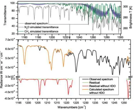
The main isotopologues of water (H16₂ O, H18₂ O and HDO) present many spectral lines in the thermal infrared region (Rothman et al., 2003; Toth, 1999). Spectral signatures of these species are well detected by IASI (Herbin et al., 2009) despite the instrument’s

5

medium spectral resolution.δ18O retrievals remain very challenging as its small vari-ations in the atmosphere require high accuracy.δD variations are larger by one order of magnitude and are therefore targeted here. Figure 1 shows part of an IASI spec-trum with the spectral windows used in the retrieval (orange curve). These have been chosen to avoid major interferences of CH4and N2O in this range.

10

3 Retrieval methodology

To retrieve δD from IASI spectral radiances we used the optimal estimation method mainly following the approach proposed by Worden et al. (2006); Schneider et al. (2006). It involves retrieving HDO and H₂O with an a priori covariance matrix which represents the variability of the two species but which also contains information on the

15

correlations between them. The retrieval performed on a log scale allows to better con-strain the solution and to minimize the error on the δD profile (Worden et al., 2006; Schneider et al., 2006; Schneider and Hase, 2011). The line-by-line-radiative transfer model software Atmosphit developed at Universit ´e Libre de Bruxelles and used in our first attempt to retrieveδD from IASI (Herbin et al., 2009) has been adapted to allow

20

this constrained approach.

While the constrained retrieval approach has been successfully applied on TES measurements (Worden et al., 2006, 2007), ground based measurements (Schnei-der et al., 2010a, 2006) and a limited number of IASI measurements (Schnei(Schnei-der and Hase, 2011), it is anticipated that the retrieval will greatly depend on the choice

25

(7)

ACPD

12, 13053–13087, 2012

IASI/MetOp

J.-L. Lacour et al.

Title Page

Tables Figures

◭ ◮

Back Close

Full Screen / Esc

Discussion

P

a

per

|

Dis

cussion

P

a

per

|

Discussion

P

a

per

|

Discussio

n

P

a

per

|

instance, Worden et al. (2012) show an improvement in the sensitivity of TES to δD after a change of the retrieval parameters.

3.1 General description

An atmospheric state vector can be related analytically to a corresponding measure-ment vector which is determined by the physics of the measuremeasure-ment. This relationship

5

can be written as

y₌F(x,b)₊ǫ, (2)

whereyis the measurement vector (in our case, the IASI radiances),ǫthe instrumental noise,xthe state vector which contains the parameters to be retrieved, andbthe one that contains all other model parameters impacting the measurement (for instance,

10

interfering species, pressure and temperature profiles).Fis the forward function. In the case of a linear problem, the maximum a posteriori solution is given by Rodgers (2000) as

ˆ

x₌x_a₊(KTS−1_ǫ K₊S_a−1)−1KTS−1_ǫ (y−Kx_a), (3)

wherex_ais the a priori state vector,Kis the Jacobian containing the partial derivative

15

of the forward model elements with respect to the state vector element

K_{i j} =∂Fi(x)

∂x_j . (4)

S_ǫ is the measurement error covariance, andSa is the a priori covariance matrix. The retrieved state is therefore a combination of the measurement and the a priori state inversely weighted by their respective covariance matrices.

20

(8)

ACPD

12, 13053–13087, 2012

IASI/MetOp

J.-L. Lacour et al.

Title Page

Tables Figures

◭ ◮

Back Close

Full Screen / Esc

Discussion

P

a

per

|

Dis

cussion

P

a

per

|

Discussion

P

a

per

|

Discussio

n

P

a

per

|

iteration of

x_i₊₁₌x_i₊(S−1_a ₊KT_i S−1_ǫ K_i)−1KT_iS−1_ǫ

[y−F(x_i)₊K_i(x_i−x_a)]. (5)

3.2 Retrieval parameters

We retrieve profiles of HDO and H16₂ O in ten discretized layers of 1 km thickness. Higher

5

altitudes are not included because in the spectral range used (from 1193 to 1223 cm−1 and from 1251 to 1253 cm−1), variations of the state vector at those altitudes do not significantly affect the measurement. This also allows for a faster retrieval. Methane (retrieved as a column) as well as surface temperature are also part of the state vector. The temperature profiles used are the ones retrieved by the Eumetsat Level 2

proces-10

sor (Schl ¨ussel et al., 2005), estimated with an error of 0.6 to 1.5 K (Pougatchev et al., 2009). Spectrally resolved emissivity values (on IASI sampling) are explicitly consid-ered above land surfaces, using the monthly climatology of Zhou et al. (2011). Only spectra not contaminated by clouds have been considered in this study.

3.3 The a priori information 15

To retrieve the state vector x from Eq. (2) is in general an ill-posed problem and to obtain a physical meaningful solution we need to constrain the retrieval with a prior information. In the optimal estimation framework, the a priori information is a measure of the knowledge of the state vector prior to the measurement. The usual approach is to assume a Gaussian distribution of the state vector, which can then be characterized

20

by a mean and covariance matrix. The covariance matrix describes to which extent parameters co-vary, for an ensemble ofnvectors{yi}. It is given by:

S_i_,_j ₌X

i,j

{(yi−y)(yj−y)}/n2. (6)

(9)

ACPD

12, 13053–13087, 2012

IASI/MetOp

J.-L. Lacour et al.

Title Page

Tables Figures

◭ ◮

Back Close

Full Screen / Esc

Discussion

P

a

per

|

Dis

cussion

P

a

per

|

Discussion

P

a

per

|

Discussio

n

P

a

per

|

Here, our state vector contains H₂O and HDO profiles. Within one profile, different altitude levels are correlated. However, there are also strong correlations between H2O and HDO. These correlations can be captured in a total covariance matrixSa, which can naturally be grouped into four sub blocks as

S_a₌





SH₂O

1

S(H₂O,HDO)

3

S(HDO,H₂O)

4

SHDO

2 

, (7)

5

where the two block S_H

2O and SHDO are the covariance matrices of the H2O and HDO, respectively. The matrices S_(H

2O,HDO)=S T

(HDO,H₂O) contain the correlations be-tween H2O and HDO.

The choice of the a priori information is critical in the regularization of an ill-posed problem (Rodgers, 2000). The best way to get adequate prior information is to derive

10

the mean and covariance from independent measurements data at high spatial resolu-tion. Only few measurements ofδD vertical profiles are available (Ehhalt, 1974; Strong et al., 2007), as are surface measurements (Galewsky et al., 2007; Johnson et al., 2011; Galewsky et al., 2011). There are however not representative for our purpose, which is to retrieveδD profiles over extended areas, covering polar to tropical latitudes.

15

Therefore, to construct a prior probability density function (pdf) we used outputs from the isotopologues-enabled general circulation model LMDz (Risi et al., 2010b) which has demonstrated its capabilities to reasonably well capture water vapor and isotopic distributions at seasonal and intra-seasonal time scales (Risi et al., 2010a, 2012b). These simulations were nudged by ECMWF reanalyzes winds to simulate a day-to-day

20

variability of weather regimes consistent with observations. Mean and covariances of HDO and H₂O profiles as well as covariances between HDO and H₂O were derived from global simulations over a whole year.

We found that the covariance matrix constructed in this way constrained the re-trieval too much. This was evident by looking at the rere-trieval residualsy−F(x,b), which

25

(10)

ACPD

12, 13053–13087, 2012

IASI/MetOp

J.-L. Lacour et al.

Title Page

Tables Figures

◭ ◮

Back Close

Full Screen / Esc

Discussion

P

a

per

|

Dis

cussion

P

a

per

|

Discussion

P

a

per

|

Discussio

n

P

a

per

|

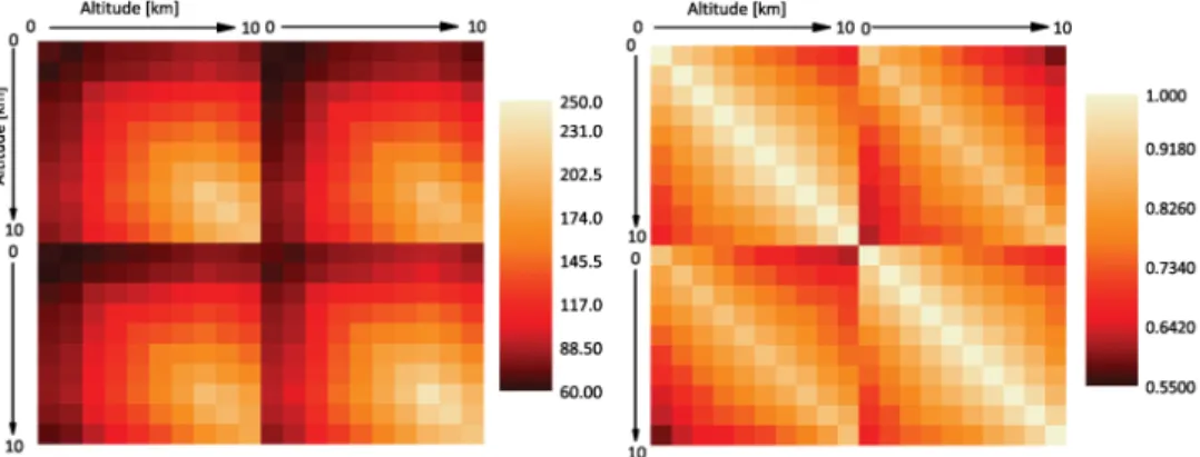
retrieval, the retrieval remains too close to the a priori, and not all available information is extracted from the spectrum. To relax the covariance matrices we slightly lowered the correlation between HDO and H2O. A simple multiplicative factor of 0.9 was applied to all elements of sub-blocks 3 and 4 in theSamatrix given by Eq. (7). Figure 2 shows the full a priori covariance matrix obtained (expressed in percent), the corresponding

5

correlation matrix is also shown. The different sub-blocks correspond to Eq. (7). From the covariance matrix one can see (diagonal elements of the first sub-block) that the variability for H₂O varies from 60 % in the first 2 km to 260 % at 7.5 km. The variability for HDO (diagonal of sub-block 3) is quite similar. The construction of the covariance matrix from global data is responsible for this large variability. The correlation matrix

10

exhibits a strong inter levels correlation for each species (sub-blocks 1 and 3).

3.4 Sensitivity diagnostic and error estimation

3.4.1 Sensitivity of the measurement

The Jacobians, which are the derivatives of the measurement vector with respect to the state vector elements (Eq. 4) describe the sensitivity of the measurement to changes

15

of the state vector. In Fig. 3, the Jacobians of HDO and H16₂ O are shown in function of altitude in the spectral window used for the retrieval. The altitudes of maximum sensi-tivities (most negative derivatives corresponding to the largest derivatives) are different for each isotopologue: for HDO maximum sensitivity is achieved between 2 and 6 km, while for H16₂ O it is at higher altitudes, between 4 and 7 km, due to saturation at lower

20

(11)

ACPD

12, 13053–13087, 2012

IASI/MetOp

J.-L. Lacour et al.

Title Page

Tables Figures

◭ ◮

Back Close

Full Screen / Esc

Discussion

P

a

per

|

Dis

cussion

P

a

per

|

Discussion

P

a

per

|

Discussio

n

P

a

per

|

3.4.2 Sensitivity of the retrieval

The averaging kernel matrix is composed of elements which are the derivatives of the estimated state ˆxwith respect to the state vectorx:

A=∂xˆ

∂x. (8)

Averaging kernels are commonly used to evaluate the sensitivity of a retrieval. The

5

matrix can be calculated for total retrieved states vectors (H₂O,HDO) but is not well defined for the calculatedδD ratio as a variation ofδD cannot uniquely be translated in variations of HDO and H2O together. Worden et al. (2006) have developed an approach to evaluate the sensitivity of their retrieval to HDO/H₂O. This approach allows for com-puting the smoothing error covariance matrix for HDO/H2O ratios from the averaging

10

kernels elements of HDO, H2O, as well as the cross terms element of the averaging kernels matrix. The covariance of the smoothing error in its general form (for the com-plete equations used in the calculation of the smoothing error of HDO/H2O retrieval, see Worden et al., 2006, Sect. 3.2) is expressed as

Sm=(A−In)Se(A−In)T, (9)

15

withS_ethe covariance matrix of a real ensemble of states generally approximated by the a priori covariance matrixSa. Equation (9) explicitly includes a vertical sensitivity through theA matrix, and it is obvious that the smoothing error decreases when av-eraging kernels are close to one and/or if the variability inS_a is small. We therefore use the ratio of the diagonal elements of the smoothing error (adapted for the joint

20

retrieval) to the diagonal elements of the a priori covariance to identify the altitude at which the retrieval is most sensitive. The results are shown in Fig. 4, they correspond to a mean error profile calculated from all error profiles across a latitudinal band. They re-veal a very strong reduction in the uncertainty after the retrieval, over the entire altitude range, but especially between 4 and 6 km.

(12)

ACPD

12, 13053–13087, 2012

IASI/MetOp

J.-L. Lacour et al.

Title Page

Tables Figures

◭ ◮

Back Close

Full Screen / Esc

Discussion

P

a

per

|

Dis

cussion

P

a

per

|

Discussion

P

a

per

|

Discussio

n

P

a

per

|

3.4.3 Error estimation from forward simulations

The error of a retrieval can be separated into 3 principal components: (1) the smoothing error, (2) the error due to uncertainties in model parameters, and (3) the error due to the measurement noise. Following this, there are two ways to conduct an error analy-sis, depending whether one considers the retrieval as an estimate of the true state with

5

an error contribution due to smoothing, or as an estimate of the true state smoothed by the averaging kernels (Rodgers, 2000). The first method requires the knowledge of a real ensemble of states in order to compute the smoothing error. Real ensemble of states are rarely available. In our case it is approximated by the a priori covariance matrix, which is characterized by a large variability, and would lead to largely

overesti-10

mating the smoothing error (see Eq. 9). Here, we therefore rather estimate errors (2) and (3). To do so, we perform retrievals on a set of simulated IASI spectra (with instru-mental noise), representative of different atmospheric conditions. More precisely, 800 spectra have been simulated with temperature and humidity (H2O and HDO) profiles ranging from standard Arctic profile to tropical standard atmospheres. These various

15

profiles have been extracted from LMDz-iso simulations. We then compared the re-trieved profiles with the real ones, smoothed with the averaging kernels to remove the contribution of the smoothing error. The smoothed profiles of water mixing ratios (q_mAK) are obtained as

log(q_mAK)=Ahh·log(qm)+(In−Ahh)·log(qp), (10)

20

(13)

ACPD

12, 13053–13087, 2012

IASI/MetOp

J.-L. Lacour et al.

Title Page

Tables Figures

◭ ◮

Back Close

Full Screen / Esc

Discussion

P

a

per

|

Dis

cussion

P

a

per

|

Discussion

P

a

per

|

Discussio

n

P

a

per

|

is

log(R_mAK)=log(R_p)

+

(Add−Ahd)·(log(HDOm)−log(HDOp)) −(Ahh−Adh)·(log(qm)−log(qp))

. (11)

5

An extensive study of the different error sources onδD retrievals from IASI (Schneider and Hase, 2011) shows that the two largest contributions to the total error are due to the measurement noise and to the uncertainty on temperature profile, while other sources of error (spectroscopy, interfering species, surface temperature and emissiv-ity) contribute to less than 4 ‰ to the total error. For our error estimation the two major

10

contributions are evaluated. First, we performed retrievals on simulated spectra with identical temperature profiles in the simulation and in the retrieval. Doing so, there is no uncertainty in the temperature profile and the errors between retrieved profiles and original ones are only due to the measurement noise. Then, to evaluate the error due to the uncertainties in the temperature profile, we performed the retrievals on simulated

15

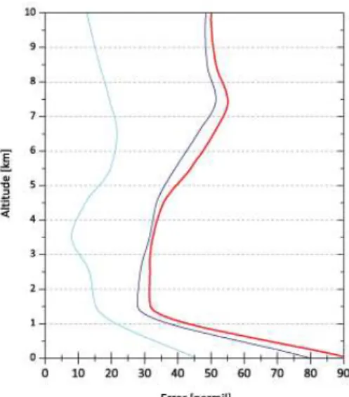
spectra with altered temperature profiles. We considered an uncertainty on the temper-ature of 1.5 K from 0 to 2 km and 0.6 K for the rest of the atmosphere, based on first validation results of the EUMETSAT L2 temperature profiles (Pougatchev et al., 2009). Differences between original and retrieved profiles give the error due to measurement noise and uncertainties in the temperature profiles, which can then be isolated. Figure 5

20

shows the total error profile expressed as the standard deviations of the difference be-tween original and retrieved profiles and its two main contributions. It shows that the total error is always below 50 ‰ in the altitude range 1–7 km, decreasing to below 40 ‰ between 2 and 5 km. The measurement noise is strongly dominating the error budget throughout the troposphere but especially above 1 km.

25

(14)

ACPD

12, 13053–13087, 2012

IASI/MetOp

J.-L. Lacour et al.

Title Page

Tables Figures

◭ ◮

Back Close

Full Screen / Esc

Discussion

P

a

per

|

Dis

cussion

P

a

per

|

Discussion

P

a

per

|

Discussio

n

P

a

per

|

with our theoretical error estimation which indicates a minimization of error between 1 and 5 km. This can be explained by the influence of the a priori covariance matrix which is more stringent in the lower atmosphere. This becomes clear when looking at the correlation between retrieved profiles and the original input profiles, which shows a maximum correlation again between 3 and 6 km.

5

4 Spatio-temporal variability ofδD retrievals

To evaluate the performance of our retrievals on real spectra, we present in this sec-tion retrievals at two sites characterized by very different hydrological regimes; namely a subsidence site (Iza ˜na) and a convective site (Darwin) for the full year 2010. In addi-tion we provideδD variations along a latitudinal gradient from−60◦ to 60◦.

10

The evaluation is carried out by comparing the retrieved δD values, and their time and spatial variations with the LMDz HDO and H2O outputs, smoothed by the averaging kernels of the retrieval (Eqs. 10 and 11). Note that due to the model grid size, the averaging kernels used here correspond to the daily mean averaging kernels of the retrievals contained in the LMDz grid box (grid size of 2.5◦ of latitude and 3.75◦ of

15

longitude). We have verified that the daily variability and the difference between land and sea averaging kernels are small enough to not a_ffect the smoothing between 3 and 6 km.

To evaluate the pattern correspondences between observations and model we first report in Table 1 some statistical diagnostics (Taylor, 2001) for the three studied cases.

20

(15)

ACPD

12, 13053–13087, 2012

IASI/MetOp

J.-L. Lacour et al.

Title Page

Tables Figures

◭ ◮

Back Close

Full Screen / Esc

Discussion

P

a

per

|

Dis

cussion

P

a

per

|

Discussion

P

a

per

|

Discussio

n

P

a

per

|

4.1 Annual and day-to-day variability at Iza ˜na and Darwin

The principal advantage of IASI over other satellite sounders measuringδD is its spatial and temporal coverage. Indeed IASI provides global coverage twice a day, which allows studying day to day variability of isotopic distributions. This is not possible with TES and SCIAMACHY instruments as they need several days to achieve global coverage.

5

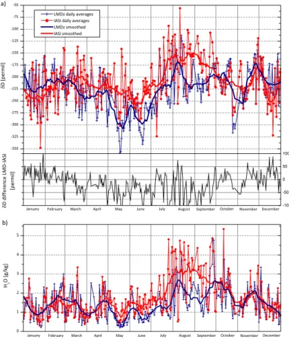
RetrievedδD and H2O time-series for the Darwin and Iza ˜na sites are shown respec-tively in Figs. 6 and 7 together with LMDz-iso simulations (blue crosses). The stud-ied zones extend from 128◦E to 133◦E, 14◦S to 10◦S for Darwin, and from 18.5◦W to 14.5◦W, 26◦N to 30◦N for Iza ˜na. Plotted values are integrated δD values for the 3–6 km layer. Daily-averaged retrieved values (full red circles) have been spatially

av-10

eraged over the model grid box. A 30 days smoothing filter applied on modeled (thick blue line) and observed (thick red line) values is also plotted to highlight the underly-ing seasonal pattern. We discuss hereafter, the seasonal variations and then the short term variations, which strongly overlap the seasonal cycle.

4.1.1 Seasonal variability 15

Darwin is a tropical site with two distinct seasons: a dry season, from May to October (Austral winter), and a wet season from November to April (Austral summer) charac-terized by cloudy and rainy conditions caused by large scale convective processes. Figure 6, which gives the 2010 time series ofδD, shows a well-marked seasonal cy-cle (80 ‰ amplitude) with lower retrieved δD values in winter (a minimum of−200 ‰

20

in June) and with high values in summer (maximum of −120 ‰ in February). This is in excellent agreement with LMDz-iso, which shows a ±95 ‰ amplitude with similar maximum in February (−130 ‰) and a minimum in June (−225 ‰). The comparison with LMDz is particularly remarkable when considering the very strong similarity in the timing and relative variations for both H2O and δD. At Darwin, the isotopic

composi-25

(16)

ACPD

12, 13053–13087, 2012

IASI/MetOp

J.-L. Lacour et al.

Title Page

Tables Figures

◭ ◮

Back Close

Full Screen / Esc

Discussion

P

a

per

|

Dis

cussion

P

a

per

|

Discussion

P

a

per

|

Discussio

n

P

a

per

|

be correlated and (2) an effect due to the convection that contributes to deplete the air mass in HDO in that case,δD and H₂O trends will be anti-correlated. This second effect is clearly visible on the Darwin time series in January-mid February where H2O reaches a maximum whileδD reaches a minimum.

Iza ˜na, located in the northern Atlantic Ocean at subtropical latitudes, is characteristic

5

of a subsidence zone with a very dry climate. The time series for Iza ˜na is shown in Fig. 7. A seasonal cycle is clearly identifiable with lowδD values in winter (min values of −250 ‰), and high values in summer (max values of−150 ‰). The general agreement between IASI and LMDz is good, but contrary to what we observed at Darwin, there are some noticeable differences in the seasonal and intra-seasonal variations. In particular,

10

the seasonality (di_fference between summer months and winter months) retrieved with IASI is larger than LMDz: in winter LMDz simulates higher δD values than IASI and in summer model simulations are lower. In annual mean this translates into a−15 ‰ bias of IASI compared to the model. While these di_fferences in δD could be due in part to the retrievals, we believe that they essentially come from the model, which has

15

been shown before to underestimate theδD seasonality in the subtropics (Risi et al., 2012b). Note that the differences do not apply to H₂O (bottom panel of Fig. 7) for which observations and simulations are in very good agreement during the winter months, but where IASI retrievals are systematically higher than the model from May to the end of September. In June, the strong increase of δD, followed by the increase of water

20

amount probably indicates that subsidence has decreased.

4.1.2 Short term variability

Figures 6 and 7 reveal strong day-to-day-variations within the broader seasonal cycle at the two locations. For instance, in a few daysδD can vary by 100 ‰ (e.g. at Darwin in June or Iza ˜na in October), which is similar to the amplitude of the seasonal cycle.

25

(17)

ACPD

12, 13053–13087, 2012

IASI/MetOp

J.-L. Lacour et al.

Title Page

Tables Figures

◭ ◮

Back Close

Full Screen / Esc

Discussion

P

a

per

|

Dis

cussion

P

a

per

|

Discussion

P

a

per

|

Discussio

n

P

a

per

|

the points) and below 25 ‰ (64 % of the points). We note however a tendency of IASI to have larger variability (for example in April–May), as further discussed below. The bias of annual mean is below 2 ‰.

At Iza ˜na, the differences are larger and vary seasonally, which is due to the seasonal bias already highlighted in Sect. 4.1.1. However, we see that LMDz-iso and IASI tend

5

to agree better in the magnitude of the variability at Iza ˜na (ratio of standard deviation of 1, see Table 1) than at Darwin, where the variability in the retrieved value (33.5 ‰) is higher by 3.5 ‰ than that from the model (30 ‰). This is also seen from Fig. 8, where retrievedδD (daily averaged value in the grid box) are plotted versus modelδD values. This figure also allows for a visualization of the correlation pattern between the two

10

di_fferent data sets. At Iza ˜na, we find a correlation coe_fficient of 0.5 (see also Table 1), when taking all observations into account. If we only consider the IASI measurements for which the daily variability in the grid box is below 35 ‰, the correlation coefficient increases to 0.64 with a slope still close to 1. At Darwin this e_ffect is not observed, the slope of 1.22 indicates a larger amplitude of the variations of IASI as compared

15

to the model (similar indication than variances ratio). The correlation coefficient is also relatively significant (0.55) here (Fig. 8 and Table 1).

Note that Yoshimura et al. (2011), have presented a similar comparison between TES retrievals and the IsoGCM model. Contrary to what we find here, they suggest that TES observations underestimate the magnitude of the short term variability. We

20

believe that the better agreement found with IASI compared to model data could be due to the specific a priori constraint applied, which could be less stringent that the one used for TES retrievals.

4.2 Spatial variability along a latitudinal gradient

In addition to the temporal variations, we have examined the ability of IASI to capture

25

(18)

ACPD

12, 13053–13087, 2012

IASI/MetOp

J.-L. Lacour et al.

Title Page

Tables Figures

◭ ◮

Back Close

Full Screen / Esc

Discussion

P

a

per

|

Dis

cussion

P

a

per

|

Discussion

P

a

per

|

Discussio

n

P

a

per

|

for the first 15 days of January 2010. As expected, the retrievedδD are largest near the equator (mean value of−140 ‰) and decrease polewards to reach a minimum value of−350 ‰ at 56◦S (gradient of−210 ‰). Local maxima are observed in the subtropics for both H2O andδD distributions but with a significant phase shift; with δD maxima being localized at higher latitudes than H₂O. This is explained by the fact that at high

5

and mid latitudes, isotopic composition follows a Rayleigh type distillation while at sub-tropical latitudes, the isotopic composition is sensitive to mixing processes, which will lead to an enrichment of the air parcel for a same water amount (Galewsky and Hurley, 2010). In the tropics the convection contributes to deplete the air masses in the heav-ier isotopologues. These processes are responsible for the smoother behavior ofδD

10

compared to H₂O.

The retrieved values are in very good agreements with model values for water vapour (correlation coefficient of 0.90, ratio of standard deviations of 1.05 and a moist bias of 0.32 g kg−1). The observed variations are in phase with the simulated ones. The only noticeable differences are the lower water concentration simulated by LMDz at the

15

equator and the higher concentration simulated in the southern subtropics.

The comparison of theδD gradients is also very good when looked at globally, with a correlation coefficient of 0.83. However, large differences occur in the magnitude of the variations (ratio of standard deviations of 1.38, LMDz standard deviation (74.02 ‰) being significant larger than IASI one (53.46 ‰)). The timing of the variations is also

20

quite good. The major differences occur in subtropical regions where LMDz systemat-ically simulates higher δD values than IASI and where correspondence between the LMDz and IASI timing is not observed. Noticeable differences also appear between 45◦ and 60◦ where LMDz values are much lower than retrieved ones, difference reaches 100 ‰ around 54◦. Added to the underestimation of the seasonality at subtropical

lati-25

(19)

ACPD

12, 13053–13087, 2012

IASI/MetOp

J.-L. Lacour et al.

Title Page

Tables Figures

◭ ◮

Back Close

Full Screen / Esc

Discussion

P

a

per

|

Dis

cussion

P

a

per

|

Discussion

P

a

per

|

Discussio

n

P

a

per

|

of the processes affectingδD in the subtropics. A detailed study of the IASI to model differences is beyond the scope of the present paper and will be the subject of forth-coming analyses.

5 Conclusions

We have described a new joint retrieval methodology for H2O and HDO from IASI

radi-5

ances spectra. Based on optimal estimation, the method is different from our previous work in that it constrains the retrievals by explicitly introducing the correlations in the concentrations of the two species inside the a priori covariance matrixS_a. It was built from a global set of daily vertical profiles from the LMDz-iso GCM representative of the whole year, and therefore shows large variability around the a priori, which are the

10

average profiles of H2O and HDO. The Sa matrix was slightly modified to decrease the model correlations between the two species. The spectral range for the retrievals was set to 1193 to 1253 cm−1 with a gap between 1223 and 1251 cm−1. With these settings, we show that IASI provides maximum sensitivity simultaneously to HDO and H2O in the free troposphere with error on the retrievedδD vertical profiles lower than

15

40 ‰ between 2 and 5 km. Considering an individual retrieval, the error onδD in the 3–6 km layer is 38 ‰ and was shown to be dominated by the measurement noise.

The seasonal variability of the IASI retrievedδD was examined at two locations for the year 2010, and compared to that of the LMDz-iso model. We found a general ex-cellent agreement in the magnitude of the seasonal pattern in comparison with the

20

model, although differences exist depending on the location. While at Iza ˜na a clear seasonal bias has been identified (overall bias of 15 ‰), the bias at Darwin is insignifi-cant (<2 ‰). Beyond the seasonal cycle, we have demonstrated the good performance of IASI to capture short-term variations ofδD (e.g. day-to-day variations) despite sig-nificant differences in the amplitude of variations estimated from the model and the

25

(20)

ACPD

12, 13053–13087, 2012

IASI/MetOp

J.-L. Lacour et al.

Title Page

Tables Figures

◭ ◮

Back Close

Full Screen / Esc

Discussion

P

a

per

|

Dis

cussion

P

a

per

|

Discussion

P

a

per

|

Discussio

n

P

a

per

|

the performance of the retrievals by analyzing the δD results for a 5◦ wide longitude band from−60◦S to 60◦N for the first 15 days of January. We show that the retrieved values are in very good agreement with the model but while the overall agreement is remarkable (correlation coe_fficient of 0.83), noticeable di_fferences occur. These are a significant deviation between LMDz and IASI at subtropical latitudes and the lowerδD

5

values simulated beyond the 45◦ latitudes. While differences highlighted in this study could be due to retrieval issues, they confirm previously documented shortcomings of the model.

More generally, the very good performance of the new retrieval method highlights fur-ther the exceptional potential of IASI to contribute to the understanding of hydrological

10

processes.

Acknowledgements. IASI has been developed and built under the responsibility of the Cen-tre National d’Etudes Spatiales (CNES, France). It is flown onboard the MetOp satellites as part of the EUMETSAT Polar System. The IASI L1 data are received through the EUMETCast near real time data distribution service. The research in Belgium was funded by the

“Commu-15

naut é Française de Belgique – Actions de Recherche Concert ées”, the Fonds National de la Recherche Scientifique (FRS-FNRS F.4511.08), the Belgian Science Policy Office and the Eu-ropean Space Agency (ESA-Prodex C90-327). L. Clarisse and P.-F. Coheur are respectively Postdoctoral Researcher (Charg é de Recherches) and Research Associate (Chercheur Qual-ifi é) with F.R.S.-FNRS. C. Clerbaux is grateful to CNES for scientQual-ific collaboration and financial

20

support.

References

Berkelhammer, M., Risi, C., Kurita, N., and Noone, D. C.: The moisture source sequence for the Madden-Julian Oscillation as derived from satellite retrievals of HDO and H₂O, J. Geophys. Res., 117, D03106, doi:10.1029/2011JD016803, 2012. 13055

25

(21)

ACPD

12, 13053–13087, 2012

IASI/MetOp

J.-L. Lacour et al.

Title Page

Tables Figures

◭ ◮

Back Close

Full Screen / Esc

Discussion

P

a

per

|

Dis

cussion

P

a

per

|

Discussion

P

a

per

|

Discussio

n

P

a

per

|

Do We Understand and Evaluate Climate Change Feedback Processes?, J. Climate, 19, 3445–3482, 2006. 13055

Clerbaux, C., Boynard, A., Clarisse, L., George, M., Hadji-Lazaro, J., Herbin, H., Hurtmans, D., Pommier, M., Razavi, A., Turquety, S., Wespes, C., and Coheur, P.-F.: Monitoring of atmo-spheric composition using the thermal infrared IASI/MetOp sounder, Atmos. Chem. Phys., 9,

5

6041–6054, doi:10.5194/acp-9-6041-2009, 2009. 13056

Craig, H.: Isotopic Variations in Meteoric Waters, Science, 133, 1702–1703, doi:10.1126/science.133.3465.1702, 1961. 13056

Ehhalt, D. H.: Vertical profiles of HTO, HDO, and H₂O in the Troposphere, NCAR-TN/STR-100, Natl. Cent. for Atmos. Res., Boulder, Colo., 1974. 13061

10

Frankenberg, C., Yoshimura, K., Warneke, T., Aben, I., Butz, A., Deutscher, N., Griffith, D., Hase, F., Notholt, J., Schneider, M., Schrijver, H., and Rockmann, T.: Dynamic Processes Governing Lower-Tropospheric HDO/H₂O Ratios as Observed from Space and Ground, Sci-ence, 325, 1374–1377, doi:10.1126/science.1173791, 2009. 13056

Frierson, D. M. W.: The Dynamics of Idealized Convection Schemes and Their

Ef-15

fect on the Zonally Averaged Tropical Circulation, J. Atmos. Sci., 64, 1959–1976, doi:10.1175/JAS3935.1, 2007. 13055

Galewsky, J. and Hurley, J. V.: An advection-condensation model for subtropical water vapor isotopic ratios, J. Geophys. Res., 115, D16116, doi:10.1029/2009JD013651, 2010. 13070 Galewsky, J., Strong, M., and Sharp, Z. D.: Measurements of water vapor D/H ratios from

20

Mauna Kea, Hawaii, and implications for subtropical humidity dynamics, Geophys. Res. Lett., 34, L22808, doi:10.1029/2007GL031330, 2007. 13061

Galewsky, J., Rella, C., Sharp, Z., Samuels, K., and Ward, D.: Surface measurements of upper tropospheric water vapor isotopic composition on the Chajnantor Plateau, Chile, Geophys. Res. Lett., 38, L17803, doi:10.1029/2011GL048557, 2011. 13061

25

Herbin, H., Hurtmans, D., Clerbaux, C., Clarisse, L., and Coheur, P.-F.: H16₂ O and HDO mea-surements with IASI/MetOp, Atmos. Chem. Phys., 9, 9433–9447, doi:10.5194/acp-9-9433-2009, 2009. 13056, 13058

Hilton, F., Armante, R., August, T., Barnet, C., Bouchard, A., Camy-Peyret, C., Capelle, V., Clarisse, L., Clerbaux, C., Coheur, P.-F., Collard, A., Crevoisier, C., Dufour, G., Edwards, D.,

30

(22)

ACPD

12, 13053–13087, 2012

IASI/MetOp

J.-L. Lacour et al.

Title Page

Tables Figures

◭ ◮

Back Close

Full Screen / Esc

Discussion

P

a

per

|

Dis

cussion

P

a

per

|

Discussion

P

a

per

|

Discussio

n

P

a

per

|

Phulpin, T., Remedios, J., Schl ¨ussel, P., Serio, C., Strow, L., Stubenrauch, C., Taylor, J., Tobin, D., Wolf, W., and Zhou, D.: Hyperspectral Earth Observation from IASI: Five Years of Accomplishments, Bull. Amer. Meteor. Soc., 93, 347–370, doi:10.1175/BAMS-D-11-00027.1, 2012. 13057

Hurtmans, D., Coheur, P.-F., Wespes, C., Clarisse, L., Scharf, O., Clerbaux, C., Hadji-Lazaro, J.,

5

George, M., and Turquety, S.: FORLI radiative transfer and retrieval code for IASI, J. Quant. Spectrosc. Rad., 113, 1391–1408, doi:10.1016/j.jqsrt.2012.02.036, 2012. 13057

Johnson, L. R., Sharp, Z. D., Galewsky, J., Strong, M., Van Pelt, A. D., Dong, F., and Noone, D.: Hydrogen isotope correction for laser instrument measurement bias at low water vapor con-centration using conventional isotope analyses: application to measurements from Mauna

10

Loa Observatory, Hawaii, Rapid Commun. Mass Sp., 25, 608–616, doi:10.1002/rcm.4894, 2011. 13061

Kang, S. M., Held, I. M., Frierson, D. M. W., and Zhao, M.: The Response of the ITCZ to Extratropical Thermal Forcing: Idealized Slab-Ocean Experiments with a GCM, J. Climate, 21, 3521–3532, doi:10.1175/2007JCLI2146.1, 2008. 13055

15

Kiehl, J. T. and Trenberth, K. E.: Earth’s Annual Global Mean Energy Budget, Bull. Amer. Meteor. Soc., 78, 197–208, doi:10.1175/1520-0477(1997)078<0197:EAGMEB>2.0.CO;2, 1997. 13055

Kurita, N., Noone, D., Risi, C., Schmidt, G. A., Yamada, H., and Yoneyama, K.: Intraseasonal isotopic variation associated with the Madden-Julian Oscillation, J. Geophys. Res., 116,

20

D24101, doi:10.1029/2010JD015209, 2011. 13055

Lee, J., Worden, J., Noone, D., Bowman, K., Eldering, A., LeGrande, A., Li, J.-L. F., Schmidt, G., and Sodemann, H.: Relating tropical ocean clouds to moist processes using water vapor isotope measurements, Atmos. Chem. Phys., 11, 741–752, doi:10.5194/acp-11-741-2011, 2011. 13055

25

Noone, D., Galewsky, J., Sharp, Z. D., Worden, J., Barnes, J., Baer, D., Bailey, A., Brown, D. P., Christensen, L., Crosson, E., Dong, F., Hurley, J. V., Johnson, L. R., Strong, M., Toohey, D., Van Pelt, A., and Wright, J. S.: Properties of air mass mixing and humidity in the subtropics from measurements of the D/H isotope ratio of water vapor at the Mauna Loa Observatory, J. Geophys. Res., 116, D22113, doi:10.1029/2011JD015773, 2011. 13055

30

(23)

ACPD

12, 13053–13087, 2012

IASI/MetOp

J.-L. Lacour et al.

Title Page

Tables Figures

◭ ◮

Back Close

Full Screen / Esc

Discussion

P

a

per

|

Dis

cussion

P

a

per

|

Discussion

P

a

per

|

Discussio

n

P

a

per

|

assessment and validation, Atmos. Chem. Phys., 9, 6453–6458, doi:10.5194/acp-9-6453-2009, 2009. 13060, 13065

Randall, D. A., Harshvardhan, Dazlich, D. A., and Corsetti, T. G.: Interactions among Radiation, Convection, and Large-Scale Dynamics in a General Circulation Model, J. Atmos. Sci., 46, 1943–1970, doi:10.1175/1520-0469(1989)046<1943:IARCAL>2.0.CO;2, 1989. 13055

5

Risi, C., Bony, S., Vimeux, F., Frankenberg, C., Noone, D., and Worden, J.: Understanding the Sahelian water budget through the isotopic composition of water vapor and precipitation, J. Geophys. Res., 115, D24110, doi:10.1029/2010JD014690, 2010a. 13056, 13061

Risi, C., Bony, S., Vimeux, F., and Jouzel, J.: Water-stable isotopes in the LMDZ4 gen-eral circulation model: Model evaluation for present-day and past climates and

applica-10

tions to climatic interpretations of tropical isotopic records, J. Geophys. Res., 115, D12118, doi:10.1029/2009JD013255, 2010b. 13057, 13061

Risi, C., Noone, D., Worden, J., Frankenberg, C., Stiller, G., Kiefer, M., Funke, B., Walker, K., Bernath, P., Schneider, M., Bony, S., Lee, J., Brown, D., and Sturm, C.: Process-evaluation of tropospheric humidity simulated by general circulation models using water vapor

iso-15

topic observations: 2. Using isotopic diagnostics to understand the mid and upper tro-pospheric moist bias in the tropics and subtropics, J. Geophys. Res., 117, D05304, doi:10.1029/2011JD016623, 2012a. 13056

Risi, C., Noone, D., Worden, J., Frankenberg, C., Stiller, G., Kiefer, M., Funke, B., Walker, K., Bernath, P., Schneider, M., Wunch, D., Sherlock, V., Deutscher, N., Griffith, D.,

20

Wennberg, P. O., Strong, K., Smale, D., Mahieu, E., Barthlott, S., Hase, F., Garc´ıa, O., Notholt, J., Warneke, T., Toon, G., Sayres, D., Bony, S., Lee, J., Brown, D., Uemura, R., and Sturm, C.: Process-evaluation of tropospheric humidity simulated by general circulation mod-els using water vapor isotopologues: 1. Comparison between modmod-els and observations, J. Geophys. Res., 117, D05303, doi:10.1029/2011JD016621, 2012b. 13056, 13061, 13064,

25

13068, 13070

Rodgers, C. D.: Inverse methods for atmospheric sounding: theory and practise, World Scien-tific, 2000. 13059, 13061, 13064

Rothman, L. S., Barbe, A., Chris Benner, D., Brown, L. R., Camy-Peyret, C., Carleer, M. R., Chance, K., Clerbaux, C., Dana, V., Devi, V. M., Fayt, A., Flaud, J. M., Gamache, R. R.,

30

(24)

ACPD

12, 13053–13087, 2012

IASI/MetOp

J.-L. Lacour et al.

Title Page

Tables Figures

◭ ◮

Back Close

Full Screen / Esc

Discussion

P

a

per

|

Dis

cussion

P

a

per

|

Discussion

P

a

per

|

Discussio

n

P

a

per

|

The HITRAN molecular spectroscopic database: edition of 2000 including updates through 2001, J. Quant. Spectrosc. Ra., 82, 5–44, 2003. 13058

Schl ¨ussel, P., Hultberg, T. H., Phillips, P. L., August, T., and Calbet, X.: The operational IASI Level 2 processor, Advances in Space Research, 36, 982–988, 2005. 13060

Schmidt, G. A., Ruedy, R. A., Miller, R. L., and Lacis, A. A.: Attribution of the present-day

5

total greenhouse effect, J. Geophys. Res., 115, D20106, doi:10.1029/2010JD014287, 2010. 13055

Schneider, M. and Hase, F.: Optimal estimation of tropospheric H₂O andδD with IASI/METOP, Atmos. Chem. Phys., 11, 11207–11220, doi:10.5194/acp-11-11207-2011, 2011. 13056, 13058, 13065

10

Schneider, M., Hase, F., and Blumenstock, T.: Ground-based remote sensing of HDO/H₂O ratio profiles: introduction and validation of an innovative retrieval approach, Atmos. Chem. Phys., 6, 4705–4722, doi:10.5194/acp-6-4705-2006, 2006. 13058

Schneider, M., Yoshimura, K., Hase, F., and Blumenstock, T.: The ground-based FTIR network’s potential for investigating the atmospheric water cycle, Atmos. Chem. Phys., 10, 3427–3442,

15

doi:10.5194/acp-10-3427-2010, 2010a. 13058

Schneider, T., O’Gorman, P. A., and Levine, X. J.: Water vapor and the dynamics of climate changes, Rev. Geophys., 48, RG3001, doi:10.1029/2009RG000302, 2010b. 13055

Sherwood, S. C., Roca, R., Weckwerth, T. M., and Andronova, N. G.: Tropospheric water vapor, convection, and climate, Rev. Geophys., 48, RG2001, doi:10.1029/2009RG000301, 2010.

20

13055

Soden, B. J. and Held, I. M.: An Assessment of Climate Feedbacks in Coupled Ocean Atmo-sphere Models, J. Climate, 19, 3354–3360, doi:10.1175/JCLI3799.1, 2006. 13055

Strong, M., Sharp, Z. D., and Gutzler, D. S.: Diagnosing moisture transport using D/H ratios of water vapor, Geophys. Res. Lett., 34, L03404, doi:10.1029/2006GL028307, 2007. 13055,

25

13061

Taylor, K. E.: Summarizing multiple aspects of model performance in a single diagram, J. Geo-phys. Res., 106, 7183–7192, doi:10.1029/2000JD900719, 2001. 13066

Toth, R. A.: HDO and D₂O low pressure, long path spectra in the 600–3100 cm−1 Region: I. HDO line positions and strengths, J. Mol. Spectrosc., 195, 73–97, 1999. 13058

30

(25)

ACPD

12, 13053–13087, 2012

IASI/MetOp

J.-L. Lacour et al.

Title Page

Tables Figures

◭ ◮

Back Close

Full Screen / Esc

Discussion

P

a

per

|

Dis

cussion

P

a

per

|

Discussion

P

a

per

|

Discussio

n

P

a

per

|

Spectrometer observations of the tropospheric HDO/H₂O ratio: Estimation approach and characterization, J. Geophys. Res., 111, D16309, doi:10.1029/2005JD006606, 2006. 13056, 13058, 13063

Worden, J., Noone, D., and Bowman, K.: Importance of rain evaporation and continental con-vection in the tropical water cycle, Nature, 445, 528–532, doi:10.1038/nature05508, 2007.

5

13055, 13056, 13058

Worden, J., Kulawik, S., Frankenberg, C., Payne, V., Bowman, K., Cady-Peirara, K., Wecht, K., Lee, J.-E., and Noone, D.: Profiles of CH₄, HDO, H₂O, and N₂O with improved lower tro-pospheric vertical resolution from Aura TES radiances, Atmos. Meas. Tech., 5, 397–411, doi:10.5194/amt-5-397-2012, 2012. 13059

10

Yoshimura, K., Frankenberg, C., Lee, J., Kanamitsu, M., Worden, J., and R ¨ockmann, T.: Comparison of an isotopic atmospheric general circulation model with new quasi-global satellite measurements of water vapor isotopologues, J. Geophys. Res., 116, D19118, doi:10.1029/2011JD016035, 2011. 13056, 13069

Zhang, R., Kang, S. M., and Held, I. M.: Sensitivity of Climate Change Induced by the

Weak-15

ening of the Atlantic Meridional Overturning Circulation to Cloud Feedback, J. Climate, 23, 378–389, doi:10.1175/2009JCLI3118.1, 2010. 13055

Zhou, D., Larar, A., Liu, X., Smith, W., Strow, L., Yang, P., Schl ¨ussel, P., and Calbet, X.: Global Land Surface Emissivity Retrieved From Satellite Ultraspectral IR Measurements, IEEE Trans. Geosci. Remote Sens, 49, 1277–1290, doi:10.1109/TGRS.2010.2051036, 2011.

20

(26)

ACPD

12, 13053–13087, 2012

IASI/MetOp

J.-L. Lacour et al.

Title Page

Tables Figures

◭ ◮

Back Close

Full Screen / Esc

Discussion

P

a

per

|

Dis

cussion

P

a

per

|

Discussion

P

a

per

|

Discussio

n

P

a

per

|

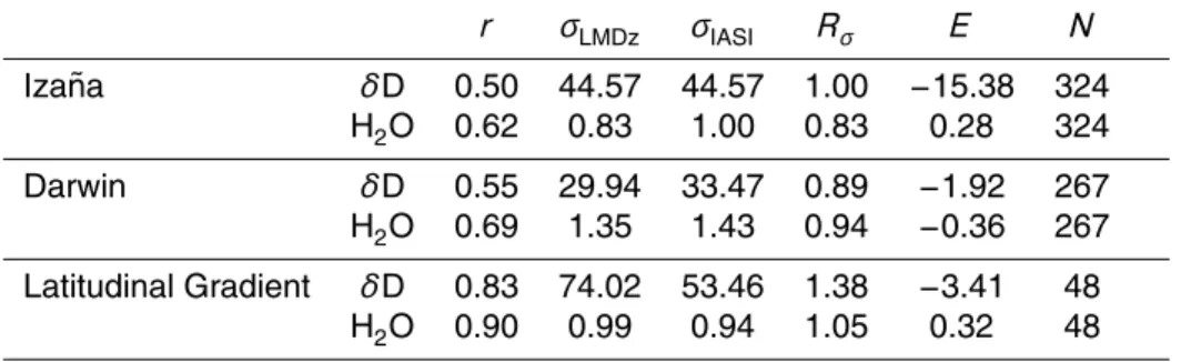
Table 1. Statistics between LMDz-iso simulated and IASI retrieved values for the different datasets presented.r is the correlation coefficient,σ_LMDzandσ_IASIare the standard deviations of LMDz-iso and IASI respectively,R_σthe ratio of standard deviations withR_σ=σ_LMDz/σ_IASI,E

is the overall bias (E=LMDz¯ −IASI), and¯ N the number of values considered. The standard deviations as the overall bias are expressed in permil and in g kg−1forδD and H₂O, respec-tively.

r σLMDz σIASI Rσ E N Iza ˜na δD 0.50 44.57 44.57 1.00 −15.38 324

H₂O 0.62 0.83 1.00 0.83 0.28 324 Darwin δD 0.55 29.94 33.47 0.89 −1.92 267 H₂O 0.69 1.35 1.43 0.94 −0.36 267 Latitudinal Gradient δD 0.83 74.02 53.46 1.38 −3.41 48

(27)

ACPD

12, 13053–13087, 2012

IASI/MetOp

J.-L. Lacour et al.

Title Page

Tables Figures

◭ ◮

Back Close

Full Screen / Esc

Discussion

P

a

per

|

Dis

cussion

P

a

per

|

Discussion

P

a

per

|

Discussio

n

P

a

per

|

(28)

ACPD

12, 13053–13087, 2012

IASI/MetOp

J.-L. Lacour et al.

Title Page

Tables Figures

◭ ◮

Back Close

Full Screen / Esc

Discussion

P

a

per

|

Dis

cussion

P

a

per

|

Discussion

P

a

per

|

Discussio

n

P

a

per

|

(29)

ACPD

12, 13053–13087, 2012

IASI/MetOp

J.-L. Lacour et al.

Title Page

Tables Figures

◭ ◮

Back Close

Full Screen / Esc

Discussion

P

a

per

|

Dis

cussion

P

a

per

|

Discussion

P

a

per

|

Discussio

n

P

a

per

|

(30)

ACPD

12, 13053–13087, 2012

IASI/MetOp

J.-L. Lacour et al.

Title Page

Tables Figures

◭ ◮

Back Close

Full Screen / Esc

Discussion

P

a

per

|

Dis

cussion

P

a

per

|

Discussion

P

a

per

|

Discussio

n

P

a

per

|

(31)

ACPD

12, 13053–13087, 2012

IASI/MetOp

J.-L. Lacour et al.

Title Page

Tables Figures

◭ ◮

Back Close

Full Screen / Esc

Discussion

P

a

per

|

Dis

cussion

P

a

per

|

Discussion

P

a

per

|

Discussio

n

P

a

per

|

(32)

ACPD

12, 13053–13087, 2012

IASI/MetOp

J.-L. Lacour et al.

Title Page

Tables Figures

◭ ◮

Back Close

Full Screen / Esc

Discussion

P

a

per

|

Dis

cussion

P

a

per

|

Discussion

P

a

per

|

Discussio

n

P

a

per

|

Fig. 6.Time series at the Darwin site for the year 2010 for the 3–6 km layer.(a)Top pannel: IASI