Interdisciplinary Study of Numerical Methods and Power Plants Engineering

(1)

Interdisciplinary Study of Numerical Methods and

Power Plants Engineering

Ioana OPRIŞ

1

1_{University POLITEHNICA of Bucharest,}_{Splaiul Independenţei 313}_{, Bucharest, Romania}

Abstract – The development of technology,

electronics and computing opened the way for a cross-disciplinary research that brings benefits by combining the achievements of different fields. To prepare the students for their future interdisciplinary approach,aninterdisciplinary teaching is adopted. This ensures their progress in knowledge, understanding and ability to navigate through different fields. Aiming

these results, the Universities introduce new

interdisciplinary courses which explore complex problems by studying subjects from different domains.

The paper presents a problem encountered in designingpower plants. The method of solvingthe problem isused to explain the numerical methods and to exercise programming.The goal of understanding a numerical algorithm that solves a linear system of equations is achieved by using the knowledge of heat transfer to design the regenerative circuit of a thermal power plant. In this way, the outcomes from the prior courses (mathematics and physics) are used to explain a new subject (numerical methods) and to advance future ones (power plants).

Keywords – interdisciplinary teaching, power plants, numerical methods, heating circuit.

1. Introduction

Interdisciplinary research between fields like science, technology, engineering, mathematics and computing is more and more necessary to solve complex problems that require cross-disciplinary analysis.

In order to face complex problems that require knowledge in several disciplines, the learning process in the universities is now adapted so as to follow interdisciplinary learning. Suchinterdisciplinary courses represent the most frequent innovation included in the revised education curricula [1].

The purpose of a specific curriculum area is achieved by using the outcomes from other curriculum areas. Moreover, the link to future subjects is prepared. This way, the curricula comes closer to the real life and the experiences of the students are more authentic [2].

Themultidisciplinary and interdisciplinary learning has the advantage of adopting a holistic approach to problems, of allowinga gradual advancement in knowledge, a deeper assimilation of the subjects, the

development of metacognitive skills and critical thinking.By combining the knowledge from several disciplines students are supported to acquire an integrated perspective and strategies focused on the practical solution. [3],[4].

2. Interdisciplinary teaching: numerical methods for the mathematical modelling of power plants

As other engineering fields, power plant engineering is more andmore combined with electronics and computing. For this reason, learning about the physical phenomena that occurs in power plants is backed by collateral knowledge of

mathematical modelling, simulation and

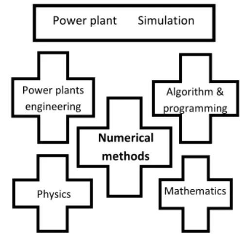
programming tools. Aiming to keep the courses on mathematics and computing as close as possible to those related to the power plants field, the outcomes of the physics courses are used to explain mathematical issues and thus to lower the gap between different courses. Furthermore, the background is prepared for the forthcoming courses on power plants. As shown in figure 1, a course on numerical methods can be considered to be at the intersection of two study directions: mathematics– simulation and physics–power plants engineering. In the end, the two directions meet again, giving to the students a sound background for the wider field of power plant simulation and computing.

Figure 1 .Courses on power plants and simulation

Mathematics Physics

Power plants engineering

Algorithm & programming

(2)

To exemplify, the paper presents a design problem for power plants that uses the outcomes of mathematics and physics to explain numerical methods and to advance the study of power plants. The problem is given at the course of numerical methods.

3. The power plant engineering problem

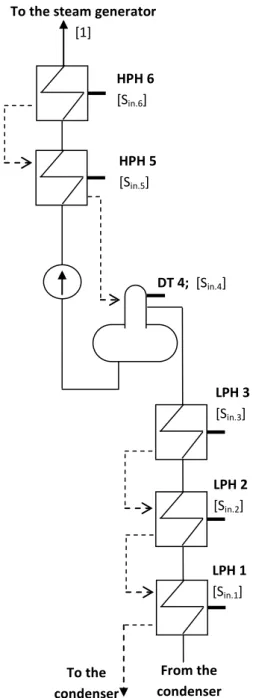
The example in figure 2 shows the feed-water regenerative circuit for a fossil-fuel power plant. The role of this circuit is to use steam extracted at different stages from the steam turbine to reheat the make-up water that enters into the steam generator. The scope of preheating the feed-water is to increase the efficiency of the thermodynamic cycle [5],[6],[7],[8].

Figure 2. A scheme for the water preheating circuit

The regenerative system shown in figure2contains three low-pressure heaters (LPH1, LPH2, LPH3), a thermal deaerator (TD) and two high-pressure heaters (HPH5, HPH6). The low-pressure and the high pressure heaters are surface heaters with the heated water flowing through the tubes and the condensing steam outside the tubes [6]. The thermal deaerator is a contact heater, in which the heated water is mixed with the condensing steam [9], [10].

The six heaters are passed by three types of fluid: - the feed-water (W), that passes the regenerative circuit on its way from the condenser to the steam generator. The water is pumped in the circuit by a feed-water pump, placed at the exit of the water from the deaerator.

- the steam (S), extracted at different pressures from the steam turbine,

- the condensate (C), obtained through the condensation of the steam in the heat-exchangers. The condensate resulted in the surface heaters flows in cascade to the heater with a lower pressure. The condensate from LPH1 is sent to the condenser. The condensed entered into the thermal deaerator is introduced into the feed-water circuit.

For this circuit, the problem consists in determining the steam flow rates extracted from the turbine, necessary at the design phase of the power plant. All the other necessary parameters of the circuit (specific enthalpies and flow rates) are known.

4. The physical description of the problem

The system of figure2is described from a physical point of view by writing the balance equations for each of the six heat exchangers [11]:

-the equation of mass conservation:

flow in=flow out

- the equation of heat conservation:

heat in= heat out.

The flow rates through the circuit are considered asspecific rates, calculated relative to the steam produced by the steam generator [12]. Considering that 1 kg of feed-water entered into the steam generator produces 1 kg of steam, the specific feed-water flow rate to the steam generator is 1.

The way in which the fluids interact within the equations of conservation differ according to the type of the heat exchanger. Their general formulation is given bellow:

HPH 6

[Sin.6]

HPH 5

[Sin.5] To the steam generator

[1]

DT 4; [Sin.4]

LPH 3

[Sin.3]

LPH 2

[Sin.2]

LPH 1

[Sin.1]

To the

condenser

(3)

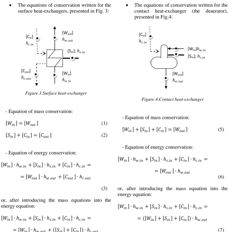
• The equations of conservation written for the surface heat-exchangers, presented in Fig. 3:

Figure 3.Surface heat-exchanger

- Equation of mass conservation:

[𝑊𝑊_{𝑖𝑖𝑖𝑖}] = [𝑊𝑊_{𝑜𝑜𝑜𝑜𝑜𝑜}] (1)

[𝑆𝑆_{𝑖𝑖𝑖𝑖}] + [𝐶𝐶_{𝑖𝑖𝑖𝑖}] = [𝐶𝐶_{𝑜𝑜𝑜𝑜𝑜𝑜}] (2)

- Equation of energy conservation:

[𝑊𝑊_{𝑖𝑖𝑖𝑖}]∙ ℎ_𝑤𝑤_._{𝑖𝑖𝑖𝑖} + [𝑆𝑆_{𝑖𝑖𝑖𝑖}]∙ ℎ_𝑠𝑠_._{𝑖𝑖𝑖𝑖} + [𝐶𝐶_{𝑖𝑖𝑖𝑖}]∙ ℎ_𝑐𝑐_._{𝑖𝑖𝑖𝑖} =

= [𝑊𝑊_{𝑜𝑜𝑜𝑜𝑜𝑜}]∙ ℎ_𝑤𝑤_._{𝑜𝑜𝑜𝑜𝑜𝑜} + [𝐶𝐶_{𝑜𝑜𝑜𝑜𝑜𝑜}]∙ ℎ_𝑐𝑐_._{𝑜𝑜𝑜𝑜𝑜𝑜}

(3)

or, after introducing the mass equations into the energy equation:

[𝑊𝑊_{𝑖𝑖𝑖𝑖}]∙ ℎ_𝑤𝑤_._{𝑖𝑖𝑖𝑖} + [𝑆𝑆_{𝑖𝑖𝑖𝑖}]∙ ℎ_𝑠𝑠_._{𝑖𝑖𝑖𝑖} + [𝐶𝐶_{𝑖𝑖𝑖𝑖}]∙ ℎ_𝑐𝑐_._{𝑖𝑖𝑖𝑖} =

= [𝑊𝑊_{𝑖𝑖𝑖𝑖}]∙ ℎ_𝑤𝑤_._{𝑜𝑜𝑜𝑜𝑜𝑜} + ([𝑆𝑆_{𝑖𝑖𝑖𝑖}] + [𝐶𝐶_{𝑖𝑖𝑖𝑖}])∙ ℎ_𝑐𝑐_._{𝑜𝑜𝑜𝑜𝑜𝑜}

(4) where:

[𝑊𝑊_{𝑖𝑖𝑖𝑖}], [𝑆𝑆_{𝑖𝑖𝑖𝑖}], [𝐶𝐶_{𝑖𝑖𝑖𝑖}]- specific flow rate of feed-water, steam, condensate entering into the heater, dimensionless;

[𝑊𝑊_{𝑜𝑜𝑜𝑜𝑜𝑜}], [𝐶𝐶_{𝑜𝑜𝑜𝑜𝑜𝑜}]- specific flow rate of feed-water, condensate at the exit of the heater,

dimensionless;

[ℎ_𝑤𝑤_._{𝑖𝑖𝑖𝑖}], [ℎ_𝑠𝑠.𝑖𝑖𝑖𝑖], [ℎ𝑐𝑐.𝑖𝑖𝑖𝑖]- specific enthalpy of

feed-water, steam, condensate entering into the heater, in kJ/kg;

[ℎ_𝑤𝑤_._{𝑜𝑜𝑜𝑜𝑜𝑜}], [ℎ_𝑐𝑐.𝑜𝑜𝑜𝑜𝑜𝑜]- specific enthalpy of feed-water,

condensate at the exit of the heater, in kJ/kg;

• The equations of conservation written for the contact heat-exchanger (the deaerator), presented in Fig.4:

Figure 4.Contact heat-exchanger

- Equation of mass conservation:

[𝑊𝑊_{𝑖𝑖𝑖𝑖}] + [𝑆𝑆_{𝑖𝑖𝑖𝑖}] + [𝐶𝐶_{𝑖𝑖𝑖𝑖}] = [𝑊𝑊_{𝑜𝑜𝑜𝑜𝑜𝑜}] (5)

- Equation of energy conservation:

[𝑊𝑊_{𝑖𝑖𝑖𝑖}]∙ ℎ_𝑤𝑤_._{𝑖𝑖𝑖𝑖} + [𝑆𝑆_{𝑖𝑖𝑖𝑖}]∙ ℎ_𝑠𝑠_._{𝑖𝑖𝑖𝑖}+ [𝐶𝐶_{𝑖𝑖𝑖𝑖}]∙ ℎ_𝑐𝑐_._{𝑖𝑖𝑖𝑖} =

= [𝑊𝑊_{𝑜𝑜𝑜𝑜𝑜𝑜}]∙ ℎ_𝑤𝑤_._{𝑜𝑜𝑜𝑜𝑜𝑜}

(6)

or, after introducing the mass equation into the energy equation:

[𝑊𝑊_{𝑖𝑖𝑖𝑖}]∙ ℎ_𝑤𝑤_._{𝑖𝑖𝑖𝑖} + [𝑆𝑆_{𝑖𝑖𝑖𝑖}]∙ ℎ_𝑠𝑠_._{𝑖𝑖𝑖𝑖}+ [𝐶𝐶_{𝑖𝑖𝑖𝑖}]∙ ℎ_𝑐𝑐_._{𝑖𝑖𝑖𝑖} =

= ([𝑊𝑊_{𝑖𝑖𝑖𝑖}] + [𝑆𝑆_{𝑖𝑖𝑖𝑖}] + [𝐶𝐶_{𝑖𝑖𝑖𝑖}])∙ ℎ_𝑤𝑤.𝑜𝑜𝑜𝑜𝑜𝑜

(7) where:

[𝑊𝑊_{𝑖𝑖𝑖𝑖}], [𝑆𝑆_{𝑖𝑖𝑖𝑖}], [𝐶𝐶_{𝑖𝑖𝑖𝑖}]- specific flow rate of feed-water, steam, condensate entering into the heater, dimensionless;

[𝑊𝑊_{𝑜𝑜𝑜𝑜𝑜𝑜}]- specific flow rate of feed-water at the exit of the heater, dimensionless;

[ℎ_𝑤𝑤_._{𝑖𝑖𝑖𝑖}], [ℎ_𝑠𝑠._{𝑖𝑖𝑖𝑖}], [ℎ_𝑐𝑐._{𝑖𝑖𝑖𝑖}]- specific enthalpy of

feed-water, steam, condensate entering into the heater, in kJ/kg;

[ℎ_𝑤𝑤_._{𝑜𝑜𝑜𝑜𝑜𝑜}]- specific enthalpy of feed-water at the exit of the heater, in kJ/kg;

After writing the equations of conservation for each heater from the scheme given in figure 2, we obtain the equations written below:

[Sin]; ℎ𝑠𝑠.𝑖𝑖𝑖𝑖

[Cout]

ℎ𝑐𝑐.𝑜𝑜𝑜𝑜𝑜𝑜

[Cin]

ℎ𝑐𝑐.𝑖𝑖𝑖𝑖

[Wout]

ℎ𝑤𝑤.𝑜𝑜𝑜𝑜𝑜𝑜

[Win]

ℎ𝑤𝑤.𝑖𝑖𝑖𝑖

[Sin]; ℎ𝑠𝑠.𝑖𝑖𝑖𝑖

[Cin]

ℎ𝑐𝑐.𝑖𝑖𝑖𝑖

[Wout]

(4)

• The balance equation written for the low pressure heater 1 (LPH 1):

[𝑊𝑊_{𝑖𝑖𝑖𝑖}_.1]∙ ℎ_𝑤𝑤_._{𝑖𝑖𝑖𝑖}_.1+ [𝑆𝑆_{𝑖𝑖𝑖𝑖}_.1]∙ ℎ_𝑠𝑠_._{𝑖𝑖𝑖𝑖}_.1+ [𝐶𝐶_{𝑖𝑖𝑖𝑖}_.1]∙ ℎ_𝑐𝑐_._{𝑖𝑖𝑖𝑖}_.1= = [𝑊𝑊_{𝑖𝑖𝑖𝑖}_.1]∙ ℎ_𝑤𝑤_._{𝑜𝑜𝑜𝑜𝑜𝑜}_.1+ ([𝑆𝑆_{𝑖𝑖𝑖𝑖}_.1] + [𝐶𝐶_{𝑖𝑖𝑖𝑖}.1])∙ ℎ𝑐𝑐.𝑜𝑜𝑜𝑜𝑜𝑜.1

(8)

[𝑊𝑊_{𝑖𝑖𝑖𝑖}_.2]∙ ℎ_𝑤𝑤_._{𝑖𝑖𝑖𝑖}_.2+ [𝑆𝑆_{𝑖𝑖𝑖𝑖}.2]∙ ℎ𝑠𝑠.𝑖𝑖𝑖𝑖.2+ [𝐶𝐶𝑖𝑖𝑖𝑖.2]∙ ℎ𝑐𝑐.𝑖𝑖𝑖𝑖.2=

= [𝑊𝑊_{𝑖𝑖𝑖𝑖}_.1]∙ ℎ_𝑤𝑤_._{𝑜𝑜𝑜𝑜𝑜𝑜}_.2+ ([𝑆𝑆_{𝑖𝑖𝑖𝑖}_.2] + [𝐶𝐶_{𝑖𝑖𝑖𝑖}_.2])∙ ℎ_𝑐𝑐_._{𝑜𝑜𝑜𝑜𝑜𝑜}_.2

(9)

[𝑊𝑊_{𝑖𝑖𝑖𝑖}_.3]∙ ℎ_𝑤𝑤_._{𝑖𝑖𝑖𝑖}_.3+ [𝑆𝑆_{𝑖𝑖𝑖𝑖}_.3]∙ ℎ_𝑠𝑠_._{𝑖𝑖𝑖𝑖}_.3=

= [𝑊𝑊_{𝑖𝑖𝑖𝑖}_.3]∙ ℎ_𝑤𝑤_._{𝑜𝑜𝑜𝑜𝑜𝑜}_.3+ [𝑆𝑆_{𝑖𝑖𝑖𝑖}_.3]∙ ℎ_𝑐𝑐_._{𝑜𝑜𝑜𝑜𝑜𝑜}_.3

(10)

• The balance equation written for the thermal deaerator (TD 4):

[𝑊𝑊_{𝑖𝑖𝑖𝑖}_.4]∙ ℎ_𝑤𝑤_._{𝑖𝑖𝑖𝑖}_.4+ [𝑆𝑆_{𝑖𝑖𝑖𝑖}_.4]∙ ℎ_𝑠𝑠_._{𝑖𝑖𝑖𝑖}_.4+ [𝐶𝐶_{𝑖𝑖𝑖𝑖}_.4]∙ ℎ_𝑐𝑐_._{𝑖𝑖𝑖𝑖}_.4=

= ([𝑊𝑊_{𝑖𝑖𝑖𝑖}.4] + [𝑆𝑆𝑖𝑖𝑖𝑖.4] + [𝐶𝐶𝑖𝑖𝑖𝑖.4])∙ ℎ𝑤𝑤.𝑜𝑜𝑜𝑜𝑜𝑜.4

(11)

• The balance equation written for the high pressure heater 5 (HPH 5):

[𝑊𝑊_{𝑖𝑖𝑖𝑖}_.5]∙ ℎ_𝑤𝑤_._{𝑖𝑖𝑖𝑖}_.5+ [𝑆𝑆_{𝑖𝑖𝑖𝑖}_.5]∙ ℎ_𝑠𝑠_._{𝑖𝑖𝑖𝑖}_.5+ [𝐶𝐶_{𝑖𝑖𝑖𝑖}_.5]∙ ℎ_𝑐𝑐_._{𝑖𝑖𝑖𝑖}_.5 = = [𝑊𝑊_{𝑖𝑖𝑖𝑖}_.5]∙ ℎ_𝑤𝑤_._{𝑜𝑜𝑜𝑜𝑜𝑜}_.5+ ([𝑆𝑆_{𝑖𝑖𝑖𝑖}_.5] + [𝐶𝐶_{𝑖𝑖𝑖𝑖}.5])∙ ℎ𝑐𝑐.𝑜𝑜𝑜𝑜𝑜𝑜.5

(12)

• The balance equation written for the high pressure heater 6 (HPH 6):

[𝑊𝑊_{𝑖𝑖𝑖𝑖}_.5]∙ ℎ_𝑤𝑤_._{𝑖𝑖𝑖𝑖}_.5+ [𝑆𝑆_{𝑖𝑖𝑖𝑖}_.5]∙ ℎ_𝑠𝑠_._{𝑖𝑖𝑖𝑖}_.5=

= [𝑊𝑊_{𝑖𝑖𝑖𝑖}_.5]∙ ℎ_𝑤𝑤_._{𝑜𝑜𝑜𝑜𝑜𝑜}_.5+ [𝑆𝑆_{𝑖𝑖𝑖𝑖}_.5]∙ ℎ_𝑐𝑐_._{𝑜𝑜𝑜𝑜𝑜𝑜}_.5

(13) The equations (8) – (13) written above form a system of linear equations, in which the unknown values are the specific steam flow rates. There are several numerical methods that can be used to solve system of linear equations [13], [14], [15].

5. The use of numerical methods for solving the problem

The linear system of six equations (8) - (13) and six unknown parameters [𝑆𝑆_{𝑖𝑖𝑖𝑖}_.1]… [𝑆𝑆_{𝑖𝑖𝑖𝑖}_.6]can be solved easily by using a numerical method [8].

For this problem, the Gauss-Jordan method is used [13].

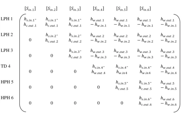
To use the method, the associated augmented matrix for the system of equations is written, by extending the coefficients matrix with a column corresponding to the free terms (table 1).

Table 1. The associated augmented matrix

[𝑆𝑆_{𝑖𝑖𝑖𝑖}_.1] [𝑆𝑆_{𝑖𝑖𝑖𝑖}_.2] [𝑆𝑆_{𝑖𝑖𝑖𝑖}_.3] [𝑆𝑆_{𝑖𝑖𝑖𝑖}_.4] [𝑆𝑆_{𝑖𝑖𝑖𝑖}_.5] [𝑆𝑆_{𝑖𝑖𝑖𝑖}_.6]

LPH 1 ℎ_𝑠𝑠_._{𝑖𝑖𝑖𝑖}_.1 -ℎ𝑐𝑐.𝑜𝑜𝑜𝑜𝑜𝑜.1

ℎ𝑠𝑠.𝑖𝑖𝑖𝑖.1 -ℎ𝑐𝑐.𝑜𝑜𝑜𝑜𝑜𝑜.1

ℎ𝑤𝑤.𝑜𝑜𝑜𝑜𝑜𝑜.1 − ℎ𝑤𝑤.𝑖𝑖𝑖𝑖.1

LPH 2

0

LPH 3

0 0

TD 4

0 0 0 ℎ𝑠𝑠

.𝑖𝑖𝑖𝑖.4 -ℎ𝑤𝑤.𝑜𝑜𝑜𝑜𝑜𝑜.4

ℎ𝑠𝑠.𝑖𝑖𝑖𝑖.4 -ℎ𝑤𝑤.𝑖𝑖𝑖𝑖4

HPH 5

0 0 0 0

ℎ𝑐𝑐.𝑖𝑖𝑖𝑖.5 -ℎ𝑐𝑐.𝑜𝑜𝑜𝑜𝑜𝑜.5

HPH 6

0 0 0 0 0

(5)

Successive operations based on pivoting are performed on the matrix, so as to transform the coefficient matrix into the identity matrix and the free terms column into a column containing the unknown values (the specific steam flow rates extracted from the turbine):

[ ] [ ]

A

=

I

S

(14)

Considering an element

a

_pp from the main diagonal of the matrix

[ ]

A

as pivot, a new matrix

[ ]

A

'

is calculated by performing the following operations [13]:

• the elements ofthe columns from the left side of the matrix remain unchanged:

ij ij

a

'

=

(15)

for

i

=

1 

(

p

−

1 )

, j=1n

• the elements of the row corresponding to the pivot are divided by the pivot:

pp pk pk

a

'

=

(16)

for

k

=

p



(

n

+

1 )

• the elements of the column corresponding to the pivot, except the pivot, are zero:

0

'

₌

kp

a

(17)

for

k

=

1 

(

p

−

1 )

,

k

=

(

p

+

1 )



n

• the other elements are calculated according to the relation:

pp ij ip

pj pp r

ij

a a a

a a

m ' = (18)

for

i

=

1 

(

p

−

1 ) (

;

p

+

1 )



n

,

(

+

1 ) (

+

1 )

=

p

n

j



After obtaining all the elements for the matrix

[ ]

A

'

, the relations (15) … (18) are used for the next pivot from the main diagonal. The same calculus is re-iterated until all the elements of the main diagonal are considered as pivot and the matrix

[ ]

I

S

is obtained.

The algorithm of the Gauss-Jordan method can be solved by the use of a computer program. After obtaining the specific steam flow rates, the steam extractions for each heat exchanger are calculated by multiplying each specific flow rate by the steam produced by the steam generator.

6. Numerical example

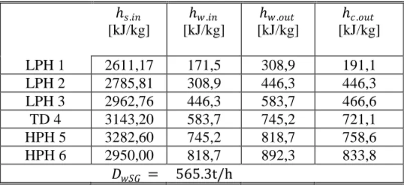
For example, the input data given in table 2.was considered for the water pre-heating scheme considered in figure 2.

The first solving step consists in building the physical description of the problem, mainly in writing the mass and heat balance equations for each heat exchanger, as described in chapter 4. The results is a system of linear equations, in which the unknown values are the specific steam flow rates.

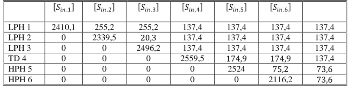
The second solving step consists in using a numerical method to solve the system of linear equations and thus model the circuit. The associated augmented matrix that resulted is given in table 3.

Table 2. Numerical example - input data

ℎ𝑠𝑠.𝑖𝑖𝑖𝑖

[kJ/kg]

ℎ𝑤𝑤.𝑖𝑖𝑖𝑖

[kJ/kg]

ℎ𝑐𝑐.𝑜𝑜𝑜𝑜𝑜𝑜

[kJ/kg]

LPH 1 2611,17 171,5 308,9 191,1

LPH 2 2785,81 308,9 446,3 446,3

LPH 3 2962,76 446,3 583,7 466,6

TD 4 3143,20 583,7 745,2 721,1

HPH 5 3282,60 745,2 818,7 758,6

HPH 6 2950,00 818,7 892,3 833,8

(6)

Table 3. Numerical example - the associated augmented matrix

[𝑆𝑆_{𝑖𝑖𝑖𝑖}_.1] [𝑆𝑆_{𝑖𝑖𝑖𝑖}_.2] [𝑆𝑆_{𝑖𝑖𝑖𝑖}_.3] [𝑆𝑆_{𝑖𝑖𝑖𝑖}_.4] [𝑆𝑆_{𝑖𝑖𝑖𝑖}_.5] [𝑆𝑆_{𝑖𝑖𝑖𝑖}_.6]

LPH 1 2410,1 255,2 255,2 137,4 137,4 137,4 137,4

LPH 2 0 2339,5 20,3 137,4 137,4 137,4 137,4

LPH 3 0 0 2496,2 137,4 137,4 137,4 137,4

TD 4 0 0 0 2559,5 174,9 174,9 137,4

HPH 5 0 0 0 0 2524 75,2 73,6

HPH 6 0 0 0 0 0 2116,2 73,6

The system was solved in MATLAB, by applying the Gauss-Jordan method. The results are presented in table 4.

Table 4. Numerical example – results

[𝑺𝑺_{𝒊𝒊𝒊𝒊}]

[-]

𝑫𝑫𝑫𝑫𝒊𝒊𝒊𝒊

[t/h]

LPH 1 0,0398 22,49

LPH 2 0,0517 29,23

LPH 3 0,0489 27,62

TD 4 0,0494 27,92

HPH 5 0,0281 15,89

HPH 6 0,0348 19,65

At this stage of learning, only the solving method is pursued, the interpretation of the values of the parameters being un-important. The main intention of the problem is to explain and understand the mechanism of using numerical methods. The knowledge of physics, mathematics and computing is recalled and reinforced, while the basis for the study of power plants engineering is given. Later, while studying power plants, the issue will be re-called and the meaning and different influences of the parameters will be studied.

7. Conclusion

Interdisciplinary learning is a good tool to teach complex problems that require knowledge in several disciplines. This is why the learning process at the universities is adapted so as to prepare the students for a holistic approach of the problems. In particular, they are prepared to use the new technologies and the increasing computing capabilities to find solutions for the engineering issues.

The paper presents an example from the field of power plants: the determination of the fixed extraction flow rates from the turbine, used for the preheating of the make-up water. This problem can be easily solved by the use of a numerical method, on the condition that one knows the physical process that occur in the circuit and the physical laws that describe it.

By solving this problem, the following main achievements are obtained:

- some notions that are already known to the students are revised (mainly, the heat transfer in heat exchangers),

- the algorithm of solving linear systems of equations by the use of numerical method is explained and exercised,

- the skills of programming and of using computer software are improved,

- the acquisition of future knowledge in the field of power plants is prepared.

By reviewing concepts from different perspectives, the knowledge and understanding are deepened and the ability to make connections beyond the boundaries of the field are developed.

References

Johnson, D. K., Ratcliff, J. L., & Gaff, J. G. (2004). A decade of change in general education. New Directions for Higher Education, 2004(125), 9-28. [1]. Borrego, M., &Newswander, L. K. (2010).

Definitions of interdisciplinary research: Toward graduate-level interdisciplinary learning outcomes. The Review of Higher Education, 34(1), 61-84.

[2]. Ivanitskaya, L., Clark, D., Montgomery, G., &Primeau, R. (2002). Interdisciplinary learning: Process and outcomes. Innovative Higher Education, 27(2), 95-111.

[3]. DeZure, D. (1999). Interdisciplinary teaching and learning. Teaching excellence: toward the best in the academy, 10(3), 1-2.

[4]. Motoiu, C. (1974). Centrale termosi hidroelectrice. Editura didactica si pedagogica, Bucuresti.

[5]. Drbal L.F., Boston P., Westra K.L., (1996), Power plant engineering, Black & Veatch.

(7)

Scientific Bulletin, Series C: Electrical Engineering, 69(4), 401-408.

[7]. Opriş I.,Cenuşă V.,Costinaş S.,Numerical Methods applied for Power Plant Calculations,Modern Computer Applications in Science and Education, WSEAS International Conference, Cambridge, USA, January (2014).

[8]. Opriş I., A deaerator Model, Recent Advances in Continuum Mechanics, Hydrology and Ecology, Energy, Environmental and Structural Engineering Series – 14, WSEAS International Conference, Rhodes Island, Greece, (2013).

[9]. Boland O., Thermal power generation, Department of Energy and Process Engineering NTNU, (2010) [10].Marinescu M., Chisacof A., Răducanu P., Motorga

A.O., Bazele termodinamiciitehnice. Transfer de căldurăşimasă – procese fundamentale, Editura

Poltehnica Press, Bucureşti, (2009).

[11].Ionescu D.C., Ulmeanu A.P., Darie G., Parteatermomecanica a centralelorelectrice. Indrumar de proiect, Editura Matrix Rom, Bucureşti, (1996).

[12].Opriş I., Metodenumerice – algoritmi de calcul,

EdituraProxima, Bucureşti, (2011).

[13].Larionescu D., Metodenumerice, EdituraTehnica, Bucuresti, (1989).

[14].Stan M., Mladin E.C., Dimitriu S., Metodenumerice,

Editura Matrix Rom, Bucureşti, (2001).

[15].Curteanu S., Iniţiereîn Matlab, Editura Polirom,

Bucureşti, (2008).

Corresponding author: Ioana Opris

Institution: University POLITEHNICA of Bucharest, Romania