www.atmos-chem-phys.net/16/5229/2016/ doi:10.5194/acp-16-5229-2016
© Author(s) 2016. CC Attribution 3.0 License.
Downscaling surface wind predictions from numerical weather
prediction models in complex terrain with WindNinja
Natalie S. Wagenbrenner1, Jason M. Forthofer1, Brian K. Lamb2, Kyle S. Shannon1, and Bret W. Butler1 1US Forest Service, Rocky Mountain Research Station, Missoula Fire Sciences Laboratory,
5775 W Highway 10, Missoula, MT 59808, USA
2Laboratory for Atmospheric Research, Department of Civil and Environmental Engineering, Washington State University, Pullman, WA 99164, USA
Correspondence to:Natalie S. Wagenbrenner ([email protected])
Received: 25 September 2015 – Published in Atmos. Chem. Phys. Discuss.: 18 January 2016 Revised: 10 April 2016 – Accepted: 14 April 2016 – Published: 27 April 2016
Abstract.Wind predictions in complex terrain are important for a number of applications. Dynamic downscaling of nu-merical weather prediction (NWP) model winds with a high-resolution wind model is one way to obtain a wind forecast that accounts for local terrain effects, such as wind speed-up over ridges, flow channeling in valleys, flow separation around terrain obstacles, and flows induced by local surface heating and cooling. In this paper we investigate the ability of a mass-consistent wind model for downscaling near-surface wind predictions from four NWP models in complex terrain. Model predictions are compared with surface observations from a tall, isolated mountain. Downscaling improved near-surface wind forecasts under high-wind (near-neutral atmo-spheric stability) conditions. Results were mixed during ups-lope and downsups-lope (non-neutral atmospheric stability) flow periods, although wind direction predictions generally im-proved with downscaling. This work constitutes evaluation of a diagnostic wind model at unprecedented high spatial reso-lution in terrain with topographical ruggedness approaching that of typical landscapes in the western US susceptible to wildland fire.
1 Introduction
Researchers from multiple disciplines rely on routine fore-casts from numerical weather prediction (NWP) models to drive transport and dispersion models, conduct wind assess-ments for wind energy projects, and predict the spread of wildfires. These applications require fine-scale, near-surface
wind predictions in regions where rugged terrain and vege-tation have a significant effect on the local flow field. Ter-rain effects such as wind speed-up over ridges, flow chan-neling in valleys, flow separation around terrain obstacles, and enhanced surface roughness alter the flow field over spa-tial scales finer than those used for routine, operational NWP forecasting.
Numerous operational mesoscale NWP model forecast products are available in real-time, such as those provided by National Centers for Environmental Prediction (NCEP). Access to these output products is facilitated by automated archiving and distribution systems such as the National Oper-ational Model Archive and Distribution System (NOMADS). These routine forecast products are highly valuable to re-searchers and forecasters, for example, as inputs to drive other models. In many cases, however, the spatial resolution of the system of interest (e.g., wildland fire spread) is much finer than that of the NWP model output.
The model grid horizontal resolution in operational NWP models is limited due to, in part, the high computational de-mands of NWP. Routine gridded forecast products are typi-cally provided at grid resolutions of 3 km or larger. The High-Resolution Rapid Refresh (HRRR) model produces 3 km output grids and is currently the highest-resolution opera-tional forecast in the US.
and Street, 2008). While successful for specific test cases, these efforts employ specialized model configurations that have not been incorporated into routine forecasting frame-works, either because they are not sufficiently robust, have not been thoroughly tested, or are too computationally in-tense for routine forecasting. For example, the configuration used in Seaman et al. (2012) is applicable for stable nocturnal conditions only.
Additionally, these modifications require technical exper-tise in NWP and access to substantial computing resources, which many consumers of NWP output do not have. Per-haps, the biggest limitation to running NWP models on grids with fine horizontal resolution is the computational demand. Time-sensitive applications, such as operational wildland fire support, require fast solution times (e.g., less than 1 h) on simple hardware (e.g., laptop computers with 1–2 proces-sors). Thus, there remains a practical need for fast-running tools that can be used to downscale coarse NWP model winds in complex terrain.
Dynamic downscaling with a steady-state (diagnostic) wind model is one option for obtaining near-surface high-resolution winds from routine NWP model output (e.g., Beaucage et al., 2014). The NWP model provides an initial wind field that accounts for mesoscale dynamics which is then downscaled by a higher resolution wind model to en-force conservation of mass and, in some cases, momentum and energy on the flow field on a higher resolution grid that better resolves individual terrain features. Dynamic down-scaling can be done in a steady-state fashion for each time step of the NWP model output. One advantage of using a steady-state downscaling approach is that the spatial resolu-tion can be increased with no addiresolu-tional computaresolu-tional cost associated with an increase in temporal resolution.
Diagnostic wind models have primarily been evaluated with observations collected over relatively simple, low-elevation hills. Askervein Hill (Taylor and Teunissen, 1987) and Bolund Hill (Berg et al., 2011) are the two mostly com-monly used data sets for evaluating diagnostic wind mod-els. These are both geometrically simple, low-elevation hills compared to the complex terrain exhibited in many regions of the western US susceptible to wildland fire. Lack of eval-uations under more complex terrain is due in part to the lack of high-resolution data sets available in complex terrain. Recently, Butler et al. (2015) reported high-resolution wind observations from a tall, isolated mountain (Big Southern Butte) in the western US. Big Southern Butte is substantially taller and more geometrically complex than both Askervein and Bolund hills.
In this work, we investigate the ability of a mass-conserving wind model, WindNinja (Forthofer et al., 2014a), for dynamically downscaling NWP model winds over Big Southern Butte. WindNinja is a diagnostic wind model de-veloped for operational wildland fire support. It is primar-ily designed to simulate mechanical effects of terrain on the flow, which are most important under high-wind conditions;
however, WindNinja also contains parameterizations for lo-cal thermal effects, which are more important under periods of weak external forcing. WindNinja has primarily been eval-uated under high-wind conditions, which are thought to be most important for wildland fire behavior, and so the thermal parameterizations have not been thoroughly tested. Wind-Ninja has previously been evaluated against the Askervein Hill data (Forthofer et al., 2014a) and found to capture impor-tant terrain-induced flow features, such as ridgetop speed-up, and it has been shown to improve wildfire spread predictions in complex terrain (Forthofer et al., 2014b).
We focus on downscaling wind in this work because it is typically more spatially and temporally variable than temper-ature or relative humidity, and thus, more important to pre-dict at high spatial resolution. Wind is also often the driving environmental variable for wildfire behavior.
The goals of this work were to (1) investigate the accuracy of NWP model near-surface wind predictions in complex ter-rain on spatial scales relevant for processes driven by local surface winds, such as wildland fire behavior and (2) assess the ability of a mass-consistent wind model to improve these predictions through dynamic downscaling. Wind predictions are investigated from four NWP models operated on differ-ent horizontal grid resolutions. This work constitutes one of the first evaluations of a diagnostic wind model with data collected over terrain with a topographical ruggedness ap-proaching that of western US landscapes susceptible to wild-land fire.
2 Model descriptions and configurations
WRF is an NWP model that solves the non-hydrostatic, fully compressible Navier-Stokes equations using finite difference method (FDM) discretization techniques (Skamarock et al., 2008). All of the NWP models investigated in this work use either the Advanced Research WRF (ARW) or the non-hydrostatic multi-scale model (NMM) core of the WRF model (Table 1).
2.1 Routine Weather Research and Forecasting (WRF-UW)
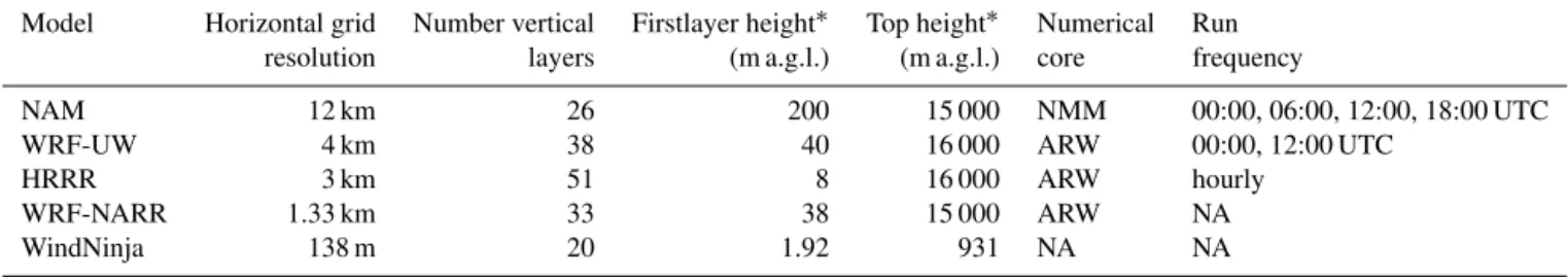
Table 1.Model specifications.
Model Horizontal grid Number vertical Firstlayer height∗ Top height∗ Numerical Run resolution layers (m a.g.l.) (m a.g.l.) core frequency
NAM 12 km 26 200 15 000 NMM 00:00, 06:00, 12:00, 18:00 UTC
WRF-UW 4 km 38 40 16 000 ARW 00:00, 12:00 UTC
HRRR 3 km 51 8 16 000 ARW hourly
WRF-NARR 1.33 km 33 38 15 000 ARW NA
WindNinja 138 m 20 1.92 931 NA NA
∗Approximate average height a.g.l.
Nevada, Utah, Wyoming, and Montana. Physical parame-terizations employed by WRF-UW include the Noah Land Surface Model (Chen et al., 1996), Thompson microphysics (Thompson et al., 2004), Kain–Fritsch convective scheme (Kain, 2004), Rapid Radiative Transfer Model (RRTM) for longwave radiation (Mlawer et al., 1997), Dudhia (1989) for shortwave radiation, and the Yonsei University (YSU) boundary layer scheme (Hong et al., 2006). WRF-UW is run at 00:00 and 12:00 UTC and generates hourly forecasts out to 84 h. The computational domain consists of 38 vertical lay-ers. The first grid layer is approximately 40 m a.g.l. and the average model top height is approximately 16 000 m a.g.l.
2.2 Weather Research and Forecasting Reanalysis (WRF-NARR)
WRF-ARW reanalysis runs were performed using the NCEP North American Regional Reanalysis (NARR) data (Mesinger et al., 2006). The reanalysis runs are referred to as WRF-NARR. The same parameterizations and grid nesting structures used in UW were also used for the WRF-NARR simulations, except that the WRF-WRF-NARR inner do-main had 33 vertical layers and a horizontal grid resolu-tion of 1.33 km (Table 1). Analysis nudging (e.g., Stauffer and Seaman, 1994) was used above the boundary layer in the outer domain (36 km horizontal grid resolution). Hourly WRF-NARR simulations were run for 15-day periods with 12 h of model spin up prior to each simulation. The first grid layer was approximately 38 m a.g.l. and the average model top height was approximately 15 000 m a.g.l. WRF-NARR differs from the other models used in this study in that it is not a routinely run model. These were custom simulations conducted by our group to provide a best-case scenario for the NWP models. Routine forecasts are already available at this resolution for limited domains (e.g., UW provides WRF simulations on a 1.33 km grid for a small domain in the Pa-cific Northwest of the US) and are likely to become more widely available at this grid resolution in the near future.
2.3 North American Mesoscale Model (NAM)
The North American Mesoscale (NAM) model is an op-erational forecast model run by NCEP for North America
(http://www.emc.ncep.noaa.gov/index.php?branch=NAM). The NAM model uses the NMM core of the WRF model. The NAM CONUS domain investigated in this study has a horizontal grid resolution of 12 km. NAM employs the Noah Land Surface model (Chen et al., 1996), Ferrier et al. (2003) for microphysics, Kain (2004) for convection, GFDL (Lacis and Hansen, 1974) for longwave and shortwave radiation, and the Mellor–Yamada–Janjic (MJF) boundary layer scheme (Janjic, 2002). The NAM model is initialized with 12 h runs of the NAM Data Assimilation System. It is run four times daily at 00:00, 06:00, 12:00, and 18:00 UTC and generates hourly forecasts out to 84 h. The computational domain consists of 26 vertical layers. The first grid layer is approximately 200 m a.g.l. and the average model top height is approximately 15000 m a.g.l. NAM forecasts are publicly available in real time from NCEP. Although the 12 km horizontal resolution used in NAM is not sufficient to resolve the butte, this resolution is sufficient for resolving the surrounding Snake River Plain and therefore can be used to generate a domain-average flow for input to WindNinja. 2.4 High-Resolution Rapid Refresh (HRRR)
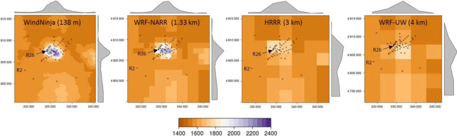
Figure 1.Terrain representation (m a.s.l.) in WindNinja, WRF-NARR, HRRR, and WRF-UW for the Big Southern Butte. Crosses indicate surface sensor locations. Maps are projected in the Universal Transverse Mercator (UTM) zone 12 coordinate system. Axis labels are eastings and northings in m. Profiles in gray are the average elevations for rows and columns in the panel. NAM (12 km) terrain is represented by just four cells and is not shown here.
2.5 WindNinja
WindNinja is a mass-conserving diagnostic wind model de-veloped and maintained by the USFS Missoula Fire Sciences Laboratory (Forthofer et al., 2014a). The theoretical formula-tion is described in detail in Forthofer et al. (2014a). Here we provide a brief overview of the modeling framework. Wind-Ninja uses a variational calculus technique to minimize the change in an initial wind field while conserving mass locally (within each cell) and globally over the computational do-main. The numerical solution is obtained using finite element method (FEM) techniques on a terrain-following mesh con-sisting of layers of hexahedral cells that grow vertically with height.
WindNinja includes a diurnal slope flow parameterization (Forthofer et al., 2009). The diurnal slope flow model used in WindNinja is the shooting flow model in Mahrt (1982). It is a one-dimensional model of buoyancy-driven flow along a slope. A micrometeorological model similar to the one used in CALMET (Scire et al., 2000; Scire and Robe, 1997) is used to compute surface heat flux, Monin-Obukhov length, and boundary layer height. The slope flow is then calculated as a function of sensible heat flux, distance to ridgetop or valley bottom, slope steepness, and surface and entrainment drag parameters. The slope flow is computed for each grid cell and added to the initial wind in that grid cell. Additional details can be found in Forthofer et al. (2009).
WindNinja was used to dynamically downscale hourly 10 m wind predictions from the above NWP models. The WindNinja computational domain was constructed from 30 m resolution Shuttle Radar Topography Mission (SRTM) data (Farr et al., 2007). The 10 m NWP winds were bilin-early interpolated to the WindNinja computational domain and used as the initial wind field. Layers above and below the 10 m height were fit to a logarithmic profile (neutral atmo-spheric stability) based on the micrometeorological model.
The computational domain consisted of 20 vertical layers. The first grid layer is 1.92 m a.g.l. and the average model top height is 931 m a.g.l.
2.6 Terrain representation
The four NWP models used in this study employ an imple-mentation of the WRF model. They use different initial and boundary conditions, incorporate different parameterizations for sub-grid processes, such as land surface fluxes, convec-tion, and PBL evoluconvec-tion, but in terms of surface wind predic-tions under the condipredic-tions investigated in this study (inland, dry summertime conditions), the horizontal grid resolution is arguably the most important difference among the models. The horizontal grid resolution affects the numerical solution since fewer terrain features are resolved by coarser grids. Coarser grids essentially impart a smoothing effect which distorts the actual geometry of the underlying terrain (Fig. 1). As horizontal cell size and terrain complexity increase, the accuracy of the terrain representation and thus, the accuracy of the near-surface flow solution deteriorate.
3 Evaluations with field observations 3.1 Observations at Big Southern Butte
Three-meter wind speeds and directions were measured with cup-and-vane anemometers at 53 locations on and around BSB. The anemometers have a measurement range of 0–44 m s−1, a resolution of 0.19 m s−1 and 1.4◦, and are accurate to within ±0.5 m s−1 and±5◦. The anemometers measured wind speed and direction every second and logged 30 s averages. We averaged these 30 s winds over a 10 min period at the top of each hour (5 min before and 5 min after the hour). The 10 min averaging period was chosen to corre-spond roughly with the timescale of wind predictions from the NWP forecasts. The NWP output is valid at a particular instant in time, but there is always some inherent temporal averaging in the predictions. The temporal averaging associ-ated with a given prediction depends on the time-step used in the NWP model and is typically on the order of minutes. The 10 min averaged observed data are referred to in the text as “hourly” observations (since they are averaged at the top of each hour) and are compared directly with the hourly model predictions.
Butler et al. (2015) observed the following general flow features at BSB. During periods of weak synoptic and mesoscale forcing (hereafter referred to collectively as “ex-ternal forcing”), the observed surface winds at BSB were de-coupled from the large-scale atmospheric flows, except for at high-elevation ridgetop locations. Diurnal slope flows dom-inated the local surface winds under periods of weak exter-nal forcing. There were frequent periods of strong exterexter-nal forcing, during which the diurnal slope winds on BSB were completely overtaken by the larger-scale winds. These peri-ods of strong external forcing at BSB were typically char-acterized by large-scale southwesterly flow aligned with the Snake River Plain, although occasionally there were also strong early morning winds from the northeast. Under peri-ods of strong external forcing wind speeds commonly varied by as much as 15 m s−1across the domain due to mechanical effects of the terrain (e.g., speed-up over ridges and lower speeds on leeward slopes). Additional details regarding the BSB field campaign can be found in Butler et al. (2015).
3.2 Evaluation methods
Hourly observations were compared against corresponding hourly predictions from the most recent model run. Mod-eled and observed winds were compared by interpolating the modeled surface wind variables to the observed surface sen-sor locations at each site. The 10 m winds from the NWP forecasts were interpolated to sensor locations, using bilinear interpolation in the horizontal dimension and a log profile in the vertical dimension. A 3-D interpolation scheme was used to interpolate WindNinja winds to the sensor locations. This 3-D interpolation was possible because the WindNinja do-main had layers above and below the surface sensor height (3.0 m a.g.l.). A 3-D interpolation scheme was not possible for the NWP domains since there were not any layers below the 3 m surface sensor height.
Model performance was quantified in terms of the mean bias, root mean square error (RMSE), and standard deviation of the error (SDE):
ϕ′= 1 N
N X
i=1
ϕ′ (1)
RMSE= " 1 N N X
i=1 ϕi′2
#1/2
(2)
SDE= "
1 N−1
N X
i=1
ϕi′−ϕ′2
#1/2
, (3)
whereϕ′ is the difference between simulated and observed variables andN is the number of observations.
3.3 Case selection
We selected a 5-day period from 15–19 July 2010 for model evaluations. This specific period was chosen because it in-cluded periods of both strong and weak external forcing, con-ditions were consistently dry and sunny, and was a period for which we were able to acquire forecasts from all NWP mod-els selected for investigation in this study.
The observed data from the 5-day period were broken into periods of upslope, downslope, and externally driven flow conditions to further investigate model performance under these particular types of flow regimes. We used the parti-tioning schemes described in Butler et al. (2015). Externally driven events were partitioned out by screening for hours dur-ing which wind speeds at a designated sensor (R2, located 5 km southwest of the butte in flat terrain) exceeded a prede-termined threshold wind speed of 6 m s−1. This sensor was chosen because it was located in flat terrain far from the butte and therefore was representative of near-surface winds that were largely unaffected by the butte itself. Hours of upslope and downslope flows (i.e., observations under weak exter-nal forcing) were then partitioned out of the remaining data. Additional details regarding the partitioning scheme can be found in Butler et al. (2015). Statistical metrics were com-puted for these 5-day periods.
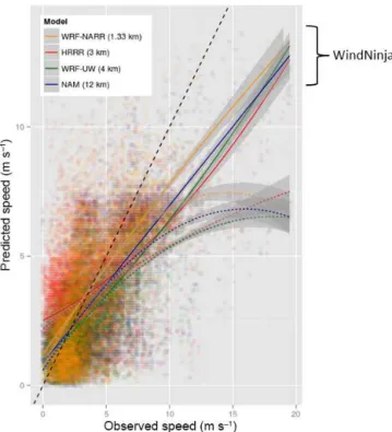
Figure 2.Observed vs. predicted wind speeds for the 5-day eval-uation period at Big Southern Butte. Dashed black line is the line of agreement. Colored lines are linear regressions (quadratic fit); dashed lines are NWP models and solid lines are NWP forecasts downscaled with WindNinja. Shading indicates 95 % confidence in-tervals.
4 Results and discussion
4.1 Overview of the 5-day simulations
Figure 2 shows observed vs. forecasted wind speeds during the 5-day period. The following generalizations can be made. The NWP models predicted wind speeds below 5 m s−1 rea-sonably well on average, although HRRR tended to over pre-dict at speeds below 3 m s−1(Fig. 2). There is a lot of scat-ter about the regression lines, but the regressions follow the line of agreement fairly well up to observed speeds around 5 m s−1. Downscaling did not improve wind speed predic-tions much in this range. NWP forecast accuracy declined for observed speeds between 5 and 10 m s−1, and accuracy sharply dropped off for observed speeds above 10 m s−1. This is indicated by the rapid departure of the NWP model regression lines from the line of agreement (Fig. 2). Down-scaling improved wind speed predictions for all NWP fore-casts for observed speeds greater than around 5 m s−1and the biggest improvements were for observed speeds greater than 10 m s−1(Fig. 2). This is indicated by the relative proximity of the downscaled regression lines to the line of agreement (Fig. 2).
Poor model accuracy at higher speeds is largely due to the models under predicting windward slope and ridgetop wind
speeds. Observed speeds at these locations were often three or four times higher than speeds in other locations in the study area (e.g., note the spatial variability in Fig. 3). But-ler et al. (2015) showed that the highest observed speeds oc-curred on upper elevation windward slopes and ridgetops and the lowest observed speeds occurred on the leeward side of the butte and in sheltered side drainages on the butte itself. Downscaling with WindNinja offers improved predictions at these locations as indicated by Fig. 2 (regression lines in closer proximity to the line of agreement) and Fig. 3 (spa-tial variability in predictions more closely matches that of the observations).
Additionally, the downscaled NAM wind speeds were as accurate as the downscaled HRRR and WRF-UW wind speeds (Fig. 2). This indicates that the NAM forecast was able to capture the important large-scale flow features around BSB such that the additional resolution provided by HRRR and WRF-UW was not essential to resolve additional flow features in the large-scale flow around BSB.
The accuracy of the NAM forecast at BSB is likely due to the fact that Snake River Plain which surrounds BSB is rela-tively flat and extends more than 50 km in all directions from the butte. Even a 12 km grid resolution would be capable of resolving the Snake River Plain and diurnal flow patterns within this large, gentle-relief drainage. Coarse-resolution models would not be expected to offer this same level of ac-curacy in areas of more extensive complex terrain, however. In areas surrounded by highly complex terrain it may be nec-essary to acquire NWP model output on finer grids in order to resolve the regional flow features.
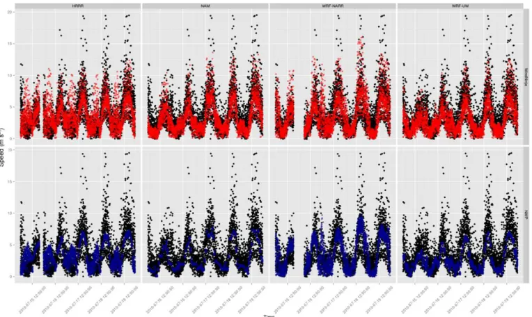
The NWP forecasts predicted the overall temporal trend in wind speed (Fig. 3), but underestimated peak wind speeds due to under predictions on ridgetops and windward slopes as previously discussed, and also occasionally in the flat terrain on the Snake River Plain surrounding the butte (Fig. 4).
NWP models with coarser resolution grids predicted less spatial variability in wind speed (Fig. 3). This is because there were fewer grid cells covering the domain, and thus fewer prediction points around the butte. The spatial variabil-ity in the downscaled wind speed predictions more closely matched that of the observed data, although the highest speeds were still under predicted (Fig. 3). Although down-scaling generally improved the spatial variability of the pre-dictions, there were cases where NWP errors clearly propa-gated into the downscaled simulations. For example, HRRR frequently over predicted morning wind speeds associated with down-drainage flow on the Snake River Plain; this er-ror was amplified in the downscaled simulations, especially at the ridgetop locations (e.g., Figs. 3–4, 15–17 July).
Figure 3.Observed (black) and predicted (colored) winds speeds at all sensors for 15–19 July 2010 at Big Southern Butte. Top panels are WindNinja predictions. Bottom panels are NWP predictions.
HRRR. Although mean bias, RMSE, and SDE in wind di-rection for the downscaled forecasts were smaller or equal to those for the NWP forecasts, the differences were small, with a maximum reduction in mean bias in wind direction of just 4◦.
It is difficult to draw too many conclusions from the spatially and temporally averaged 5-day statistics, however, since this period included a range of meteorological condi-tions (e.g., high-wind events from different direccondi-tions, ups-lope flow, downsups-lope flow) each of which could have been predicted with a different level of skill by the models. Quali-tatively, however, the 5-day results demonstrate that the spa-tial variability in the downscaled winds better matches that of the observed winds at BSB (Fig. 3) and, although the re-ductions were small in some cases, nearly all statistical met-rics also improved with downscaling. The analysis is broken down by flow regime in the next section for more insight into model performance.
4.2 Performance under Upslope, downslope, and externally forced flows
Local solar heating and cooling was a primary driver of the flow during the slope flow regime at BSB (Butler et al., 2015), with local thermal effects equal to or exceeding the
local mechanical effects of the terrain on the flow. Because there is weak external forcing (i.e., input wind speeds to WindNinja are low), the downscaling is largely driven by the diurnal slope flow parameterization in WindNinja during the slope flow regimes.
During upslope flow, the diurnal slope flow parameteriza-tion increases speeds on the windward slopes and reduces speeds (or reverses flow and increases speeds, depending on the strength of the slope flow relative to the prevailing flow) on lee slopes due to the opposing effects of the prevailing wind and the thermal slope flow. The parameterization has the opposite effect during downslope flow; windward slope speeds are reduced (or possibly increased if downslope flow is strong enough to reverse the prevailing flow) and lee side speeds are enhanced.
4.2.1 Wind speed
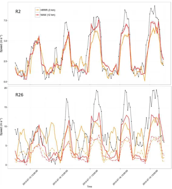
Figure 4.Observed (black line) and predicted (colored lines) wind speeds for sensor R2 located 5 km southwest of Big Southern Butte on the Snake River Plain and sensor R26 located on a ridgetop. Dashed colored lines are NWP models and solid colored lines are WindNinja.
of the butte (Figs. 6–8). Since WindNinja is designed primar-ily to simulate the mechanical effects of the terrain on the flow, it is during these high-wind events that the downscal-ing has the most opportunity to improve predictions across the domain. This has important implications for wildfire ap-plications since high-wind events are often associated with increased fire behavior.
The NWP models tended to under predict wind speeds on the windward slopes, ridgetops, and surrounding flat terrain, and over predict on the lee side of the butte during high wind events (e.g., Fig. 6). The largest NWP errors in wind speed during high wind events were on the ridgetops, where speed-up occurred and the NWP under predicted speeds. These largest wind speed errors were reduced by downscaling (e.g., Fig. 6). Downscaling reduced NWP wind speed errors in most regions on the butte, although the general trend of
un-der predicting wind speeds on the windward side and over predicting on the lee side did not change (e.g., Fig. 6).
There were consistent improvements in predicted wind speeds from downscaling during the upslope regime, al-though the improvements were smaller than for the exter-nally driven regime (Fig. 5). Wind speeds were lower dur-ing the slope flow regimes than durdur-ing the externally forced regime (Figs. 6–8), and thus, smaller improvements were possible with downscaling. There was some speed-up pre-dicted on the windward side of the butte during the represen-tative upslope case which appeared to match the observed wind field (Fig. 8).
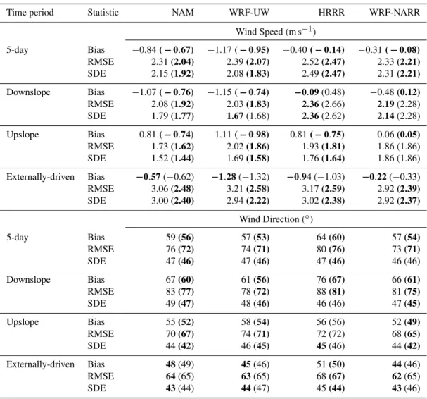
Table 2.Model mean bias, root mean square error (RMSE), and standard deviation of errors (SDE) for surface wind speeds and directions during the 5-day evaluation period at Big Southern Butte. Downscaled values are in parentheses. Smaller values are in bold. The 5-day period includes the Downslope, Upslope, and Externally driven time periods.
Time period Statistic NAM WRF-UW HRRR WRF-NARR
Wind Speed (m s−1)
5-day Bias −0.84(−0.67) −1.17(−0.95) −0.40(−0.14) −0.31(−0.08)
RMSE 2.31(2.04) 2.39(2.07) 2.52(2.47) 2.33(2.21)
SDE 2.15(1.92) 2.08(1.83) 2.49(2.47) 2.31(2.21)
Downslope Bias −1.07(−0.76) −1.15(−0.74) −0.09(0.48) −0.48(0.12)
RMSE 2.08(1.92) 2.03(1.83) 2.36(2.66) 2.19(2.28)
SDE 1.79(1.77) 1.67(1.68) 2.36(2.62) 2.14(2.28)
Upslope Bias −0.81(−0.74) −1.11(−0.98) −0.81(−0.75) 0.06(0.05)
RMSE 1.73(1.62) 2.02(1.86) 1.93(1.81) 1.86 (1.86)
SDE 1.52(1.44) 1.69(1.58) 1.76(1.64) 1.86 (1.86)
Externally-driven Bias −0.57(−0.62) −1.28(−1.32) −0.94(−1.03) −0.22(−0.33)
RMSE 3.06(2.48) 3.21(2.58) 3.17(2.59) 2.92(2.39)
SDE 3.00(2.40) 2.94(2.22) 3.02(2.38) 2.92(2.37)
Wind Direction (◦)
5-day Bias 59(56) 57(53) 64(60) 57(54)
RMSE 76(72) 74(71) 80(76) 73(71)
SDE 47(46) 47(46) 47(46) 46 (46)
Downslope Bias 67(60) 61(56) 76(67) 66(61)
RMSE 83(77) 78(72) 88(81) 81(75)
SDE 49(47) 48(46) 46 (46) 47(45)
Upslope Bias 55(52) 58(54) 56 (56) 52(49)
RMSE 70(67) 74(71) 72 (72) 68(65)
SDE 44(42) 46(45) 45(46) 44(42)
Externally-driven Bias 48(49) 45(46) 51(50) 44(46)
RMSE 64(65) 63(65) 68(67) 62(65)
SDE 43(44) 44(47) 45(44) 43(46)
is partly due to the fact that HRRR tended to over predict early morning winds associated with down drainage flows on the Snake River Plain. These errors were amplified by the downscaling, especially at ridgetop locations (Fig. 4). In real-ity, the high-elevation ridgetop locations tended to be decou-pled from lower-level surface winds during the slope flow regimes due to flow stratification. WindNinja assumes neu-tral atmospheric stability, however, so this stratification is not handled. A parameterization for non-neutral atmospheric conditions is currently being tested in WindNinja.
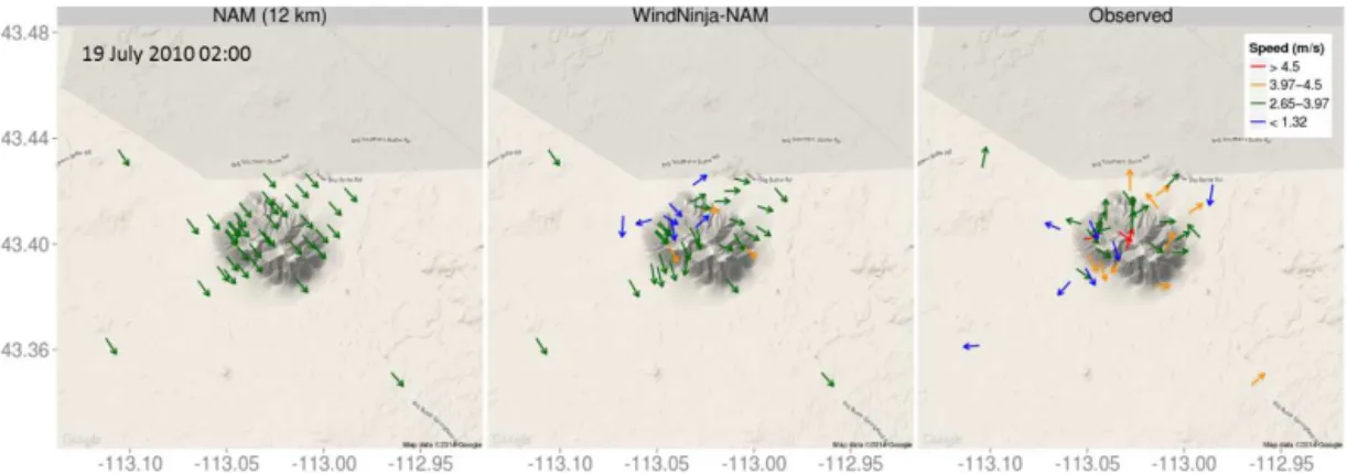
The diurnal slope flow parameterization in WindNinja re-sulted in lower speeds on the windward side and higher speeds on the lee side of the butte for the representative downslope case (Fig. 7). These downscaled speeds better matched those of the observed wind field, although speeds were still under predicted for ridgetops and a few other lo-cations around the butte (Fig. 7). The high observed speeds at the ridgetop locations are not likely due to thermal slope flow effects, but could be from the influence of gradient-level
winds above the nocturnal boundary layer. These ridgetop locations are high enough in elevation (800 m above the sur-rounding plain) that they likely protruded out of the nocturnal boundary layer and were exposed to the decoupled gradient-level winds. Butler et al. (2015) noted that ridgetop winds did not exhibit a diurnal pattern and tended to be decoupled from winds at other locations on and around the butte. Lack of diurnal winds at the summit of the butte is also confirmed by National Oceanic and Atmospheric Administration Field Research Division (NOAA-FRD) mesonet station data col-lected at the top of BSB (described in Butler et al., 2015; http://www.noaa.inel.gov/projects/INLMet/INLMet.htm).
Figure 5.Root-mean-square error in wind speed (left) and wind direction (right) at Big Southern Butte for the 5-day evaluation period (N=4149), and downslope (N=1593), upslope (N=717), and externally driven (N=966) periods within the 5-day period. Sample size: N=number of hours×number of sensor locations.
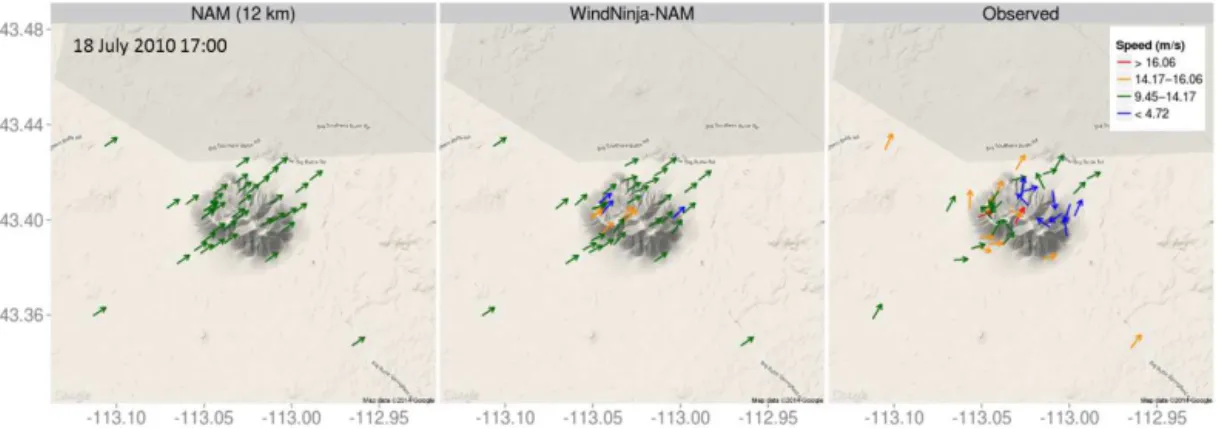
Figure 6.Predicted and observed winds for an externally forced flow event at Big Southern Butte.
model used. The slope flow parameterization is being evalu-ated in a companion paper.
4.2.2 Wind direction
The biggest improvement in wind direction predictions from downscaling occurred during the downslope regime (Fig. 5). Wind direction improved with downscaling for all NWP models during periods of downslope flow. This indicates that the diurnal slope flow model helped to orient winds downslope. This is confirmed by inspection of the vector plots for the representative downslope case which show the downscaled winds oriented downslope on the southwest and northeast faces of the butte (Fig. 7). Downscaling reduced speeds on the northwest (windward) side of the butte, but did not predict strong enough downslope flow in this region
to reverse the flow from the prevailing northwest direction (Fig. 7). This again suggests that perhaps the diurnal slope flow algorithm is predicting overly weak slope flows.
Wind direction predictions during the upslope regime also improved with downscaling for all NWP models except HRRR (Fig. 5). Downscaled winds for the representative up-slope case were oriented upup-slope on the southwest (lee side) of the butte and matched the observed winds in this region well (Fig. 8). This is an improvement over the NWP wind directions on the lee side of the butte.
wind-Figure 7.Predicted and observed winds for a downslope flow event at Big Southern Butte.
Figure 8.Predicted and observed winds for an upslope flow event at Big Southern Butte.
ward side of the butte, but not on the leeward side, where the observed field indicates some recirculation in the flow field (Fig. 6). The prevailing southwesterly flow is captured by the NWP model, but the lee side recirculation is not. Wind-Ninja does not predict the lee side recirculation, and thus, the downscaling does not improve directions on the lee side of the butte (Fig. 7). This is an expected result, as WindNinja has been shown to have difficulties simulating flows on the lee side of terrain features due to the fact that it does not account for conservation of momentum in the flow solution (Forthofer et al., 2014a).
5 Summary
The horizontal grid resolutions of NWP models investigated in this study were too coarse to resolve the BSB terrain. Re-sults showed that the NWP models captured the important large-scale flow features around BSB under most conditions, but were not capable of predicting the high spatial variabil-ity (scale of 100s of meters) in the observed winds on and around the butte induced by mechanical effects of the terrain and local surface heating and cooling. Thus, surface winds from the NWP models investigated in this study would not be sufficient for forecasting wind speeds on and around the
butte at the spatial scales relevant for processes driven by lo-cal surface winds, such as wildland fire spread.
Wind predictions generally improved for all NWP mod-els by downscaling with WindNinja. The biggest improve-ments occurred under high-wind events (near-neutral atmo-spheric stability) when observed wind speeds were greater than 10 m s−1. This finding has important implications for fire applications since increased wildfire behavior is often associated with high winds. Downscaled NAM wind speeds were as accurate as downscaled WRF-UW and HRRR wind speeds, indicating that an NWP model with 12 km grid res-olution was sufficient for capturing the large-scale flow fea-tures around BSB.
Results indicated that WindNinja predicted overly weak slope flows compared to observations. Weak slope flow could be caused by several different issues within the diurnal slope flow parameterization in WindNinja: improper parameteri-zation of surface or entrainment drag parameters, poor esti-mation of the depth of the slope flow, or deficiencies in the micrometeorological model. These issues will be explored in future work.
This work constitutes evaluation of a diagnostic wind model at unprecedented high spatial resolution and ter-rain complexity. While extensive evaluations have been per-formed with data collected in less rugged terrain (e.g., Askervein Hill and Bolund Hill, relatively low-elevation hills with simple geometry), to our knowledge, this study is the first to evaluate a diagnostic wind model with data collected in terrain with topographical ruggedness approaching that of typical landscapes in the western US susceptible to wildland fire. This work demonstrates that NWP model wind fore-casts can be improved in complex terrain, especially under high-wind events, through dynamic downscaling via a mass-conserving wind model. These improvements should prop-agate on to more realistic predictions from other model ap-plications which are sensitive to surface wind fields, such as wildland fire behavior, local-scale transport and dispersion, and wind energy applications.
Acknowledgements. Thanks to Dave Ovens and Cliff Mass of the University of Washington for providing access to the WRF-UW simulations and Eric James of NOAA–GSD Earth System Research Laboratory for access to the HRRR simulations. Thanks to Serena Chung of the Laboratory for Atmospheric Research, Washington State University, for guidance on the WRF-NARR simulations. We also thank the participants in the BSB field campaign, in-cluding Dennis Finn, Dan Jimenez, Paul Sopko, Mark Vosburgh, Larry Bradshaw, Cyle Wold, Jack Kautz, and Randy Pryhorocky.
Edited by: T. Garrett
References
Beaucage, P., Brower, M. C., and Tensen, J.: Evaluation of four nu-merical wind flow models for wind resource mapping, Wind En-ergy, 17, 197–208, 2014.
Berg, J., Mann, J., Bechmann, A., Courtney, M. S., and Jor-gensen, H. E.: The Bolund experiment, Part I: flow over a steep, three-dimensional hill, Bound.-Lay. Meteorol., 141, 219–243, 2011.
Butler, B. W., Wagenbrenner, N. S., Forthofer, J. M., Lamb, B. K., Shannon, K. S., Finn, D., Eckman, R. M., Clawson, K., Brad-shaw, L., Sopko, P., Beard, S., Jimenez, D., Wold, C., and Vos-burgh, M.: High-resolution observations of the near-surface wind field over an isolated mountain and in a steep river canyon, At-mos. Chem. Phys., 15, 3785–3801, doi:10.5194/acp-15-3785-2015, 2015.
Chen, F., Mitchell, K., Schaake, J., Xue, Y., Pan, H., Koren, V., Duan, Y., Ek, M., and Betts, A.: Modeling of land-surface evap-oration by four schemes and comparison with FIFE observa-tions, J. Geophys. Res., 101, 7251–7268, 1996.
Ching, J., Rotunno, R., LeMone, M., Martilli, A., Kosovic, B., Jimenez, P. A., and Dudhia, J.: Convectively induced secondary circulations in fine-grid mesoscale numerical weather prediction models, Mon. Weather Rev., 142, 3284–3302, 2014.
Chou, M. and Suarez, M. J.: An Efficient Thermal Infrared Radi-ation ParameterizRadi-ation for Use in General CirculRadi-ation Models, Technical Report Series on Global Modeling and Data Assimila-tion, NASA/Goddard Space Flight Center, Greenbelt, MD, USA, NASA Tech. Memo. 104606, 3, 85 pp., 1994.
Chow, F. K. and Street, R. L.: Evaluation of turbulence closure models for large-eddy simulation over complex terrain: flow over Askervein Hill, J. Appl. Meteorol. Clim., 48, 1050–1065, 2008. Dudhia, J.: Numerical study of convection observed during the
winter monsoon experiment using a mesoscale two-dimensional model, J. Atmos. Sci., 46, 3077–3107, 1989.
Farr, T. G., Rosen, P. A., Caro, E., Crippen, R., Duren, R., Hens-ley, S., Kobrick, M., Paller, M., Rodriguez, E., Roth, L., Seal, D., Shaffer, S., Shimada, J., Umland, J., Werner, M., Oskin, M., Bur-bank, D., and Alsdorf, D.: The Shuttle Radar Topography Mis-sion, Rev. Geophys., 45, RG2004, doi:10.1029/2005RG000183, 2007.
Ferrier, B., Lin, Y., Parrish, D., Pondeca, M., Rogers, E., Manikin, G., Ek., M., Hart, M., DiMego, G., Mitchell, K., Chuang, H.-Y.: Changes to the NCEP Meso Eta analysis and forecast system: modified cloud microphysics, assimilation of GOES cloud-top pressure, assimilation of NEXRAD 88D radial wind velocity data, NWS Technical Procedures Bulletin, 25 pp., Silver Spring, MD, USA, 2003.
Forthofer, J., Shannon, K., and Butler, B.: Simulating diur-nally driven slope winds with WindNinja, in: Eighth Sympo-sium on Fire and Forest Meteorology, 13–15 October 2009, Kalispell, MT, 156275, available at: https://ams.confex.com/ ams/8Fire/techprogram/paper_156275.htm (last access: 11 De-cember 2015), 2009.
Forthofer, J. M., Butler, B. W., and Wagenbrenner, N. S.: A com-parison of three approaches for simulating fine-scale winds in support of wildland fire management: Part I. Model formulation and accuracy, Int. J. Wildland Fire, 23, 969–981, 2014a. Forthofer, J. M., Butler, B. W., McHugh, C. W., Finney, M. A.,
Bradshaw, L. S., Stratton, R.D, Shannon, K. S., and Wagenbren-ner, N. S.: A comparison of three approaches for simulating fine-scale surface winds in support of wildland fire management, Part I I. An exploratory study of the effect of simulated winds on fire growth simulations, Int. J. Wildland Fire, 23, 982–994, 2014b. Hong, S.-Y., Noh, Y., and Dudhia, J.: A new vertical diffusion
pack-age with an explicit treatment of entrainment, Mon. Weather Rev., 134, 2318–2341, 2006.
Janjic, Z.: Nonsingular Implementation of the Mellor–Yamada Level 2.5 Scheme in the NCEP Meso Model, NCEP Office Note No. 437, 61, Camp Springs, MD, 2002.
Kain, J.: The Kain–Fritsch convective parameterization: an up-date, J. Meteor. Climatol., 43, 170–181, 2004.
Lundquist, K. A., Chow, F. K., and Lundquist, J. K.: An immersed boundary method for the Weather Research and Forecasting Model, Mon. Weather Rev., 138, 796–817, 2010.
Mahrt, L.: Momentum balance of gravity flows, J. Atmos. Sci., 39, 2701–2711, 1982.
Mesinger, F., DiMego, G., Kalnay, E., Mitchell, K., Shafran, P. C., Ebisuzaki, W., Jovic, D., Woollen, J., Rogers, E., Berbery, E. H., Ek, M. B., Fan, Y., Grumbine, R., Higgins, W., Li, H., Lin, Y., Manikin, G., Parrish, D., and Shi, W.: North American regional reanalysis, B. Am. Meteorol. Soc., 87, 343–360, 2006.
Mlawer, E. J., Taubman, S. J., Brown, P. D., Iacono, M. J., and Clough, S. A.: Radiative transfer for inhomogenous atmospheres: RRTM, a validated correlated-k model for the longwave, J. Geo-phys. Res., 102, 16663–16682, 1997.
Scire, J. S. and Robe, F. R.: Fine-Scale Application of the CALMET Meteorological Model to a Complex Terrain Site, Air & Waste Management Associations’s 90th Annual Meeting & Exhibition 1997, Toronto, Ontario, Canada, 16 pp., 1997.
Scire, J. S., Robe, F. R., Fernau, M. E., and Yamartino, R. J.: A User’s Guide for the CALMET Meteorological Model, Earth Tech, Inc., Concord, MA, available at: src.com/calpuff/ download/CALMET_UsersGuide.pdf (last access: 11 December 2015), 2000.
Seaman, N. L., Gaudet, B. J., Stauffer, D. R., Mahrt, L., Richard-son, S. J., Zielonka, J. R., and Wyngaard, J. C.: Numerical pre-diction of submesoscale flow in the nocturnal stable boundary layer over complex terrain, Mon. Weather Rev., 140, 956–977, 2012.
Skamarock, W. C., Klemp, J. B., Dudhia, J., Gill, D. O., Barker, D. M., Duda, M. G., Huang, X., Wang, W., and Pow-ers, J. G.: A Description of the Advanced Research WRF Version 3, NCAR Tech. Note NCAR/TN-475STR, Boulder, CO, USA, 2008.
Smirnova, T. G., Brown, J.M, and Benjamin, S. J.: Performance of different soil model configurations in simulating ground surface temperature and surface fluxes, Mon. Weather Rev., 125, 1870– 1884, 1997.
Smirnova, T. G, Brown, J. M., Benjamin, S. G., and Kim, D.: Parameterization of cold season processes in the MAPS land-surface scheme, J. Geophys. Res., 105, 4077–4086, 2000. Stauffer, D. R. and Seaman, N. L.: Multiscale four-dimensional data
assimilation, J. Appl. Meteorol., 33, 416–434, 1994.
Taylor, P. A. and Teunissen, H. W.: The Askervein Hill project: overview and background data, Bound.-Lay. Meteorol., 39, 15– 39. 1987.