Imaging gravity waves in lower stratospheric AMSU-A radiances, Part 2: Validation case study

www.atmos-chem-phys.net/6/3343/2006/ © Author(s) 2006. This work is licensed under a Creative Commons License.

Chemistry

and Physics

Imaging gravity waves in lower stratospheric AMSU-A radiances,

Part 2: Validation case study

S. D. Eckermann1, D. L. Wu2, J. D. Doyle3, J. F. Burris4, T. J. McGee4, C. A. Hostetler5, L. Coy1, B. N. Lawrence6, A. Stephens6, J. P. McCormack1, and T. F. Hogan3

1_{E. O. Hulburt Center for Space Research, Naval Research Laboratory, Washington, D.C., USA} 2_{Jet Propulsion Laboratory, California Institute of Technology, Pasadena, California, USA} 3_{Marine Meteorology Division, Naval Research Laboratory, Monterey, CA, USA}

4_{NASA Goddard Space Flight Center, Greenbelt, MD, USA} 5_{NASA Langley Research Center, Hampton, VA, USA}

6_{British Atmospheric Data Center, Rutherford Appleton Laboratory, Oxfordshire, UK} Received: 30 November 2005 – Published in Atmos. Chem. Phys. Discuss.: 27 March 2006 Revised: 3 August 2006 – Accepted: 5 August 2006 – Published: 14 August 2006

Abstract. Two-dimensional radiance maps from Channel 9 (∼60–90 hPa) of the Advanced Microwave Sounding Unit (AMSU-A), acquired over southern Scandinavia on 14 Jan-uary 2003, show plane-like oscillations with a wave-lengthλhof∼400–500 km and peak brightness temperature

amplitudes of up to 0.9 K. The wave-like pattern is observed in AMSU-A radiances from 8 overpasses of this region by 4 different satellites, revealing a growth in the disturbance amplitude from 00:00 UTC to 12:00 UTC and a change in its horizontal structure between 12:00 UTC and 20:00 UTC. Forecast and hindcast runs for 14 January 2003 using high-resolution global and regional numerical weather prediction (NWP) models generate a lower stratospheric mountain wave over southern Scandinavia with peak 90 hPa temperature am-plitudes of∼5–7 K at 12:00 UTC and a similar horizontal wavelength, packet width, phase structure and time evolu-tion to the disturbance observed in AMSU-A radiances. The wave’s vertical wavelength is∼12 km. These NWP fields are validated against radiosonde wind and temperature pro-files and airborne lidar propro-files of temperature and aerosol backscatter ratios acquired from the NASA DC-8 during the second SAGE III Ozone Loss and Validation Experiment (SOLVE II). Both the amplitude and phase of the strato-spheric mountain wave in the various NWP fields agree well with localized perturbation features in these suborbital mea-surements. In particular, we show that this wave formed the type II polar stratospheric clouds measured by the DC-8 li-dar. To compare directly with the AMSU-A data, we convert these validated NWP temperature fields into swath-scanned brightness temperatures using three-dimensional Channel 9 weighting functions and the actual AMSU-A scan patterns from each of the 8 overpasses of this region. These

NWP-Correspondence to:S. D. Eckermann

(stephen.eckermann@nrl.navy.mil)

based brightness temperatures contain two-dimensional os-cillations due to this resolved stratospheric mountain wave that have an amplitude, wavelength, horizontal structure and time evolution that closely match those observed in the AMSU-A data. These comparisons not only verify grav-ity wave detection and horizontal imaging capabilities for AMSU-A Channel 9, but provide an absolute validation of the anticipated radiance signals for a given three-dimensional gravity wave, based on the modeling of Eckermann and Wu (2006).

1 Introduction

This improved resolution and accuracy should allow AMSU-A to resolve finer-scale atmospheric features than earlier instruments. One focus of investigation has been stratospheric gravity waves, which are poorly resolved by most satellite remote-sensing instruments. Wu (2004) was the first to investigate this possibility experimentally by iso-lating along-track fluctuations in radiances acquired from AMSU-A stratospheric channels at various cross-track scan angles. Global maps of these variances in the extratropi-cal Southern Hemisphere showed enhancements over moun-tains and at the edge of the polar vortex that resembled simi-larly enhanced radiance variances from the Microwave Limb Sounder (MLS) on the Upper Atmosphere Research Satel-lite (UARS). Since the MLS radiance variance is known to originate from resolved gravity wave oscillations (e.g., McLandress et al., 2000; Jiang et al., 2004), these correla-tions appear to show AMSU-A resolving stratospheric grav-ity waves.

Whereas MLS cyclically stares at or scans the limb, AMSU-A cyclically scans the atmosphere beneath the satel-lite at 30 equispaced off-nadir cross-track viewing angles be-tween±48.33◦. As the satellite orbits, this scanning pattern sweeps out two-dimensional “pushbroom” images of atmo-spheric radiances beneath the satellite, rather than the one-dimensional horizontal cross sections from MLS. Wu and Zhang (2004) isolated small-scale structure in AMSU-A ra-diances at all 30 scan angles and plotted these perturbations at the measurement locations to yield a swath-scanned hori-zontal image of the perturbation field. Focusing on a region off the northeastern coast of the USA on 19–21 January 2003, they found plane-wave-like oscillations that appeared to cap-ture the horizontal struccap-ture of stratospheric gravity waves radiated from the jet stream.

While correlations between AMSU-A radiance perturba-tions and wave fluctuaperturba-tions observed in MLS radiances (Wu, 2004) or simulated by a mesoscale model (Wu and Zhang, 2004) certainly suggest that AMSU-A can resolve gravity waves, they do not provide quantitative insights into why and how wave signals manifest in these data. To provide some theoretical insight, Eckermann and Wu (2006) devel-oped a simplified model of the in-orbit acquisition of radi-ances by AMSU-A Channel 9 on both the NOAA and EOS Aqua satellites. The three-dimensional temperature weight-ing functions that this modelweight-ing generated were in turn used to specify how gravity waves with different temperature am-plitudes, horizontal propagation directions, and vertical and horizontal wavelengths manifested as oscillatory signals in swath-scanned Channel 9 radiance imagery. These simula-tions indicated that a lower stratospheric gravity wave which had a temperature amplitude of&3 K, a vertical wavelength of &10 km, and a horizontal wavelength of &150–200 km should appear as a detectable oscillation in Channel 9 bright-ness temperatures (i.e., above the nominal ±0.2 K noise floor). If any of these threshold criteria is not met, the grav-ity wave is probably not visible to AMSU-A Channel 9. The

simulations also showed how these resolved radiance signals, when mapped horizontally, provided a two-dimensional im-age of the wave’s horizontal structure, with some cross-track distortions introduced due to the limb effect and variations in footprint diameters versus scan angle.

These predicted amplitude and wavelength thresholds for gravity wave detection by AMSU-A Channel 9 provide the same basic guidance as previous modeling studies for other satellite instruments (e.g., McLandress et al., 2000; Preusse et al., 2002; Jiang et al., 2004). They are important in spec-ifying the kinds of waves being measured and what infor-mation these data can and cannot provide (see, e.g., Alexan-der, 1998; Wu et al., 2006). However, this AMSU-A forward model provides important additional guidance.

First, it models how two-dimensional gravity wave struc-ture is both imaged horizontally and distorted in swath-scanned AMSU-A radiances. Horizontal gravity wave imag-ing is an important new satellite measurement capability, heretofore only hinted at by a few limited observational case studies (Dewan et al., 1998; Wu and Zhang, 2004) and never previously modeled. Second, if the three-dimensional wave-length and amplitude structure of the gravity wave is known, the forward model of Eckermann and Wu (2006) makes spe-cific predictions about the absolute brightness temperature amplitudes that should be seen by Channel 9. Indeed, given a complete gridded three-dimensional temperature field, the forward model can convert these temperatures into bright-ness temperature maps that can be compared directly with the AMSU-A data. Previous models of the visibility charac-teristics of specific satellite instruments have only been used to crudely filter model-generated wave fields, so that the rel-ative variations in observed and modeled wave variances can be more meaningfully compared, such as geographical and seasonal variability (McLandress et al., 2000; Jiang et al., 2002, 2004). No study to date has converted model-predicted gravity wave fields into absolute radiance oscillations whose amplitudes and phases can be compared directly with the ob-served radiance oscillations.

NWP-based radiance perturbations are compared to those measured by AMSU-A, to assess how closely the observed horizontal structure, wavelengths, amplitudes and time evo-lution of the measured fluctuations are reproduced.

2 Data sources

2.1 Advanced Microwave Sounding Unit-A

Since the companion paper of Eckermann and Wu (2006) provides a description of AMSU and develops a model of its Channel 9 stratospheric radiance acquisition, here we pro-vide only a brief summary of the salient features of this in-strument for this observational study.

AMSU-A has 15 measurement channels, 6 of which (Channels 9–14) are stratospheric temperature channels. Channels 9 though 14 sample wing line thermal oxygen emissions centered at 57.290 GHz. The one-dimensional (1-D) vertical weighting functions at nadir for these channels peak progressively higher in the stratosphere, from∼90 hPa for Channel 9 though to∼2.5 hPa for Channel 14 (Kidder et al., 2000). We analyze only Channel 9 radiances in this study.

The AMSU-A cross-track scanning pattern consists of

j=1. . .30 sequential step-and-stare measurements at eq-uispaced off-nadir beam anglesβj between ±48.33◦,

dis-tributed symmetrically about the subsatellite point: see Fig. 1 of Eckermann and Wu (2006). The cross-track swath width at stratospheric altitudes is∼2100 km for the NOAA satel-lites. Each scan cycle takes 8 s to complete, so that data from successive scans are separated by∼60 km along track given a 7.4 km s−1satellite velocity. At the near-nadir beam positionsj=15,16, the half-power horizontal measurement footprints are nearly circular with diameters of∼48 km for Channel 9 on the NOAA satellites. These footprints become broader and more elliptically elongated cross-track at the off-nadir measurement angles (Kidder et al., 2000; Eckermann and Wu, 2006). Swath widths and footprint diameters are somewhat smaller for the AMSU-A on EOS Aqua due to its lower orbit altitude of 705 km compared to 833 km for the NOAA satellites (see Fig. 6 of Eckermann and Wu, 2006). The altitude of peak Channel 9 sensitivity increases with in-creasing|βj| due to the limb effect (Goldberg et al., 2001;

Eckermann and Wu, 2006), to a maximum peak altitude of

∼65 hPa at the outermost scan angles (Fig. 1b; see also Fig. 4 of Eckermann and Wu, 2006). Here we analyze raw radi-ances to which no limb adjustment procedures (Goldberg et al., 2001) have been applied.

2.2 NASA DC-8 lidar data

The Langley Research Center (LaRC) aerosol lidar operates in comanifested form with the Goddard Space Flight Center (GSFC) Airborne Raman Ozone, Temperature and Aerosol Lidar (AROTAL) on NASA’s DC-8 research aircraft. The

0.0 0.5 1.0 1.5 2.0 2.5 3.0

∆Zk (km)

0 10 20 30 40 50

altitude (km)

NOGAPS-ALPHA L60 ECMWF IFS L60 COAMPS L85

(a)

(b)

0 0.25 0.5

Wj(Z)

j = 15,16 j = 1,30

1000 100 10 1

pressure (hPa)

Fig. 1. (a)Vertical layer thicknesses1Zk of various NWP model levels. COAMPS altitudes and thicknesses are geometric heights for a surface altitude of 0 km, whereas NOGAPS-ALPHA and ECMWF IFS altitudes and thicknesses are pressure heights assum-ing a scale height of 7 km and a nominal sea-level surface pressure of 1013.25 hPa. (b)AMSU-A Channel 9 1-D vertical weighting functionsWj(Z)for the near-nadir beams (j=15,16) and far off-nadir beams (j=1,30) from Eckermann and Wu (2006).

lidars transmit vertically and collect backscattered radiation with a zenith-viewing telescope.

The GSFC/LaRC lidar emits laser pulses at 1064, 532, and 355 nm, the fundamental, doubled, and tripled frequencies, respectively, from a neodymium:yttrium/aluminum/garnet (Nd:YAG) laser. Here we study aerosol backscatter ra-tios (ABRs) derived from GSFC/LaRC lidar backscatter at 1064 nm,

S1064=

βaerosol+βair

βair

, (1)

whereβaerosolandβair are the backscatter coefficients from aerosol and air molecules, respectively. The lidar measures the total backscatterβaerosol+βair:βairis derived using atmo-spheric densities from meteorological analyses along track. GSFC/LaRC lidar ABRs are issued at 75 m vertical resolu-tion every∼15 s.

Stratospheric ABRs provide first–order discrimination among different types of polar stratospheric clouds (PSCs). PSC-free regions yieldS1064∼1. Type I PSCs, composed of nitric acid trihydrate (NAT, type Ia) or supercooled ternary solutions (STS, type Ib) yield S1064∼3–30, whereas type II PSCs (ice) yield S1064∼50–500 (e.g., Fueglistaler et al., 2003).

21–22 s at a vertical resolution of 150 m from just above the aircraft to∼60 km altitude, though the intrinsic temporal and vertical data resolutions are somewhat coarser (Burris et al., 2002a).

3 Models

3.1 Numerical weather prediction models

To validate specific gravity waves resolved in AMSU-A ra-diances, we would ideally compare directly with suborbital measurements of the wave field. However, to model grav-ity wave-induced fluctuations in the AMSU-A radiances ad-equately, we need to know the full three-dimensional (3-D) structure of the wave field (Eckermann and Wu, 2006). Sub-orbital gravity wave data are much too sparse to characterize gravity waves three-dimensionally, yet without this informa-tion these two data sets cannot be meaningfully compared and cross-validated.

Thus, to provide the necessary 3-D wave fields that can link the AMSU-A and suborbital measurements, we ana-lyze output from three different numerical weather prediction (NWP) models, each of which bring some unique capabili-ties to our validation study. All of these models were run at high spatial resolution in order to explicitly resolve any long wavelength gravity wave activity that AMSU-A might be sensitive to.

3.1.1 ECMWF IFS

We use forecast and analysis fields issued operationally by the European Centre for Medium-Range Weather Forecasts (ECMWF) Integrated Forecast System’s (IFS) TL511L60 global spectral model (Ritchie et al., 1995; Untch and Hor-tal, 2004). We use global gridpoint fields on all 60 hybrid

σ-pvertical model levels from the surface to 0.1 hPa issued on the reduced N256 linear Gaussian grid that progressively thins the number of points around a latitude circle, from 1024 at the equator to 192 at±80◦latitude. Forecasts and analyses are available every 6 h, starting at 00:00 UTC.

3.1.2 NOGAPS-ALPHA

Since the six hourly output from the ECMWF IFS proves too sparse for precise comparisons with AMSU-A data, we per-formed hindcasts using high resolution Navy NWP models.

Global NWP for the U.S. Department of Defense (DoD) is provided by the Naval Research Laboratory’s (NRL) Navy Operational Global Atmospheric Prediction System (NOGAPS), which is run operationally at the Fleet Nu-merical Meteorology and Oceanography Center (FNMOC) (Hogan and Rosmond, 1991). Here we use a developmen-tal version of the NOGAPS global spectral forecast model with Advanced Level Physics and High Altitude

(NOGAPS-ALPHA: Eckermann et al., 2004; McCormack et al., 2004; Allen et al., 2006).

The NOGAPS-ALPHA hindcasts performed here used a “cold start” procedure in which global analyzed winds and geopotential heights on reference pressure levels and a 1◦×1◦ grid are read in and interpolated to the model’s quadratic Gaussian grid and hybridσ-plevels. Initial model temperatures are computed hydrostatically from the geopo-tentials. The model was then forwarded in time without meteorological assimilation update cycles. To initialize our runs for January 2003 at altitudes below 10 hPa, two different Navy analyses were available: (a) archived operational anal-ysis from the then-operational Navy multivariate optimum interpolation (MVOI) system (Barker, 1992); (b) reanaly-sis fields for this period from the NRL Atmospheric Vari-ational Data Assimilation System (NAVDAS) (Daley and Barker, 2001), which assimilated AMSU-A radiances from the NOAA 15 and 16 satellites. NAVDAS with AMSU-A ra-diance assimilation became operational at FNMOC on 9 June 2004 and has significantly improved NOGAPS forecast skill (Baker et al., 2005; Allen et al., 2006). While NOGAPS-ALPHA runs using both analyses were performed and ana-lyzed for cross-validation purposes, here we will only show results from runs initialized with the NAVDAS reanalysis.

From 10–0.4 hPa we initialized using FNMOC’s opera-tional “STRATOI” analysis (see Sect. 4 of Goerrs and Phoe-bus, 1992), whose primary data source is ATOVS temper-ature retrievals issued by NOAA’s National Environmental Satellite, Data and Information Service (NESDIS) (Reale et al., 2004). From 0.4–0.005 hPa we have no Navy anal-ysis fields available for January 2003 (STRATOI was ex-tended to 0.1 hPa in June 2003). Thus we extrapolated the 0.4 hPa STRATOI fields upwards by progressively relax-ing them with increasrelax-ing altitude to zonal-mean climatolog-ical winds from the UARS Reference Atmosphere Project (URAP; Swinbank and Ortland, 2003) and temperatures from the 1986 COSPAR International Reference Atmosphere (CIRA; Fleming et al., 1990): for algorithm details, see Eck-ermann et al. (2004). This final global initial state is adjusted within NOGAPS-ALPHA for hydrostatic balance then run through a nonlinear normal mode filter (Errico et al., 1988), to suppress potential for any spurious gravity wave genera-tion due to unbalanced initial condigenera-tions. Surface ice con-centrations, land/sea surface temperatures and snow depths are also initialized using FNMOC analysis and are updated from archived analysis every 12 h in our model runs.

waves from the model top. We saved model fields spectrally every hour. Gridpoint fields were obtained by retransform-ing onto the 720×360 quadratic Gaussian grid (∼0.5◦ reso-lution) at all 60 modelσ-plevels.

3.1.3 COAMPS

NRL’s Coupled Ocean/Atmosphere Mesoscale Prediction System (COAMPS®) is FNMOC’s regional operational NWP system (Hodur, 1997). COAMPS hindcast runs here used two nested 169×169 horizontal grids of 30 km and 10 km horizontal grid spacing, and 85 nonuniformly-spaced terrain-following vertical levels (Gal-Chen and Somerville, 1975) extending to a top geometric altitude of 33 km (see Fig. 1a). The top several kilometers contained a numerical sponge layer to absorb upward-propagating gravity waves at the upper boundary. As for the NOGAPS-ALPHA runs, we performed separate COAMPS runs initialized in a cold-start procedure using archived MVOI analyses and NAVDAS re-analyses, with output from the latter runs only analyzed in this study. Archived NOGAPS forecast fields were used to specify the lateral boundary conditions every 6 h. Output fields were saved every hour on the intrinsic model grid.

The primary purpose of the COAMPS runs is to provide higher resolution fields than the global models in order to resolve gravity wave fields better. Thus, subsequent analysis will focus only on the high horizontal resolution 10×10 km2 fields from the nested COAMPS run.

3.2 AMSU-A radiance acquisition model

To relate gravity waves in the three-dimensional gridded NWP temperature fieldsT with those observed in Channel 9 AMSU-A brightness temperaturesTB, we convert

tempera-tures into a model brightness temperature field

TBNWP(Xj, Yj)= Z Z Z

Wj(X−Xj, Y−Yj, Z)

T (X, Y, Z)dXdY dZ, (2) using the three-dimensional AMSU-A weighting functions

Wj(X, Y, Z)from the modeling study of Eckermann and Wu

(2006). Following their notation (see their Fig. 1),XandY

are along-track and cross-track distances, respectively,Z is pressure altitude,j is beam position (as defined by its cross-track scan angleβj: see Sect. 2.1), and (Xj,Yj) is the

loca-tion of the peakWj(X, Y, Z)response which we take to be

the measurement location. Equation (2) is integrated over the full range of permissableX,Y andZvalues.

To evaluate Eq. (2) numerically, we must regrid the NWP temperatures from their longitude, latitude and terrain-following vertical levels onto the same regular Cartesian

(X, Y, Z)grid used forWj(X, Y, Z). The next 4 paragraphs

explain how we do this.

First, we vertically interpolate the NWP temperature fields onto a regular pressure height grid of1Z=0.5 km, a choice

based on the minimum intrinsic vertical model resolutions in Fig. 1a. Weighting functionsWj(X, Y, Z)are interpolated

onto this same vertical grid.

For a given scan cycle, each of thej=1. . .30 AMSU-A radiance measurements comes registered at its ground-level footprint longitudeλˆj and latitudeφˆj. Using spherical

ge-ometry (see Fig. 16 of Eckermann and Wu, 2006), we cor-rect these locations by moving along the line-of-sight ray from the surface to the∼60–90 hPa altitude where the rele-vant weighting functionWj(X, Y, Z)peaks. The NWP fields

are distributed at gridpoints (λˆi,φˆi). For each AMSU-A

measurement at beam position j, we compute great circle distancesdi,j from these gridpoints (λˆi,φˆi) to this beam’s

(corrected) footprint location (λˆj,φˆj). We retain model

tem-peraturesT (λˆi,φˆi, Z)only at those gridpointsi for which di,j≤300 km. Since AMSU-A footprint radii are<100 km

at every beam position (Eckermann and Wu, 2006), grid-point fields more than 300 km from the peak of the weight-ing function can be safely discarded as lyweight-ing well outside this beam’s field of view. This process significantly thins the NWP field and speeds up the subsequent numerical compu-tation of Eq. (2).

Next the scan axes (X,Y) must be specified on the sphere. The Y-axis vector direction is computed as the bearing angle

γj,ssfrom true north from the subsatellite point for this scan,

(λˆss,φˆss), to the current footprint location (λˆj,φˆj). Yj is

the great circle distancedj,ssbetween (λˆj,φˆj) and (λˆss,φˆss),

andXj=0 (since AMSU-A does not scan along-track). For

the negative scan anglesβj, we setYj=−dj,ss.

To regrid the retained NWP temperatures T (λˆi,φˆi, Z)

onto the (X,Y) grid, we compute great circle distancesdi,ss

between all the retained gridpoints i and the subsatellite point, as well as their bearing anglesγi,ssfrom the

subsatel-lite point. We use these di,ss andγi,ss values to compute

corresponding coordinates (Xi, Yi) using Napier’s Rules for

spherical right-angled triangles. After triangulating all the

(Xi, Yi)data, we linearly interpolate the temperatures at each

level onto a regular (X,Y) grid of length 380 km and resolu-tion 5 km in both direcresolu-tions centered at (Xj, Yj).

With T (X, Y, Z) and Wj(X, Y, Z) now on a common

(X, Y, Z) grid, we evaluate Eq. (2) numerically using rectan-gular integration over this entire gridded(X, Y, Z)domain.

4 Radiances and temperatures over Scandinavia on 14

January 2003

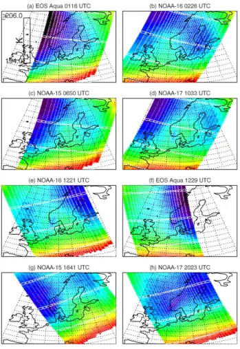
Figure 2 plots AMSU-A Channel 9 brightness tempera-turesTB(λˆj,φˆj)acquired during the ascending and

Fig. 2. AMSU-A Channel 9 brightness temperaturesTB(λˆj,φˆj) measured during the ascending and descending overpasses of Scan-dinavia by EOS Aqua, NOAA-15, NOAA-16, and NOAA-17. These values (in Kelvin) are plotted as color-coded footprint el-lipses at the measurement location: see color bar in panel(a). White curves outline these measurement footprints for every tenth scan. Panels are arranged in chronological order, with the universal time and satellite platform of the overpass given in the plot title.

the Channel 9 radiance acquisition model of Eckermann and Wu (2006): see their Fig. 6.

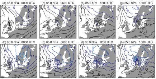
Figure 3 plots the 6-hourly ECMWF IFS analysis temper-atures for 14 January 2003 at 85 hPa and 65 hPa, the approx-imate vertical range of the peak AMSU-A weighting func-tion responses at various beam posifunc-tions (see Fig. 1b). Like the brightness temperatures, the analysis temperatures tran-sition from warmer mid-latitude values to much colder val-ues in and around Scandinavia. McCormack et al. (2004) showed that the very cold stratospheric temperatures over Scandinavia on 14 January 2003 were driven by adiabatic up-lift from an anticyclonic upper-tropospheric ridge over West-ern Europe and a weak wave-1 stratospheric disturbance that pushed the vortex core off the pole towards Scandinavia. These vortex disturbances presaged a minor stratospheric warming, which split the vortex about a week later

(McCor-mack et al., 2004) and shut off much of the early season PSC formation and ozone loss chemistry (Feng et al., 2005).

Despite gross similarites, variations in the brightness tem-perature maps from measurement to measurement in Fig. 2 do not correlate obviously with the analysis temperatures in Fig. 3. Since adjacent AMSU-A measurements can be separated by an hour or less, the 6-hourly resolution of the ECMWF analysis temperatures is too coarse to investigate these variations systematically, and so we turn now to hourly temperature fields from the NOGAPS-ALPHA runs.

Figure 4 plots hindcast NOGAPS-ALPHA temperatures at times and altitudes corresponding to those plotted in Fig. 3. The geographical structure and temporal evolution are very similar to the ECMWF analysis fields. In the “cold pool” re-gions, NOGAPS-ALPHA shows a cold bias of∼1–2 K rel-ative to the ECMWF analysis, which originates mostly from the NAVDAS fields used for initialization (not shown), which have a 1–2 K cold bias relative to the ECMWF analysis in these cold-pool regions. Apart from this the comparison is very good, even down to details in the small-scale temper-ature oscillations over southern Scandinavia and Scotland, which we will focus on subsequently.

Next, we compute synthetic brightness temperature fields

TBNWP(λˆj,φˆj)from these NOGAPS-ALPHA temperatures by evaluating Eq. (2) via the methods outlined in Sect. 3.2. For each AMSU-A measurement in Fig. 2, we evaluate Eq. (2) using the hourly NOGAPS-ALPHA temperature field closest in time to this satellite overpass. Results are plotted in Fig. 5.

Synthetic NOGAPS-ALPHA brightness temperatures in each panel of Fig. 5 compare very well in both magnitude and horizontal structure with the corresponding AMSU-A data in Fig. 2. This indicates that most of the panel-to-panel differences in Fig. 2 do not originate from biases among the various instruments deployed on different satellite platforms. Rather, most of the variability comes from the limb effect, which causes the far off-nadir measurements at the edges of the cross-track swaths to peak at∼65 hPa, while those near-nadir measurements in the middle of the swath peak nearer 85 hPa (Goldberg et al., 2001; Eckermann and Wu, 2006).

Thus, for example, the very cold brightness temperatures at 01:16 UTC to the west of Scandinavia in Figs. 2a and 5a can be understood in terms of far off-nadir measurements at the edge of the swath that measure the compact core of cold 65 hPa temperatures in Fig. 4b. The overpass 1 h later in Figs. 2b and 5b measured warmer brightness tem-peratures here since it sampled this region with near-nadir beams which measured the significantly warmer 85 hPa tem-peratures in Fig. 4a, while the off-nadir beams sampled the warmer 65 hPa temperatures located either side of this cold core in Fig. 4b.

(a) 85.0 hPa 0000 UTC 198 200 202 202 202 202 204 204 206 206 208 208

(b) 65.0 hPa 0000 UTC

194 196 198 200 200 202 202 204 204 206

(c) 85.0 hPa 0600 UTC

200 200 200 202 202 202 202 202 204 204 204 206 206 208

(d) 65.0 hPa 0600 UTC

196 196 198 198 198 200 200 200 200 ₂₀₂ 202 204 204 206

(e) 85.0 hPa 1200 UTC₂₀₀

200 202 202 202 202 204 204 204 204 206 206 206 208

(f) 65.0 hPa 1200 UTC

196 196 198 198 200 202 202 202 204 204

(g) 85.0 hPa 1800 UTC

198 200 202 202 204 204 204 206 206 208 210

(h) 65.0 hPa 1800 UTC

194 196 198 200 202 ₂₀₄ 204 206 206

Fig. 3. ECMWF IFS TL511L60 6-hourly analysis temperatures for 14 January 2003 at 85 hPa (top row) and 65 hPa (bottom row),

corre-sponding roughly to the peak altitudes of the near-nadir and far off-nadir Channel 9 weighting functions, respectively. Contour interval is 2 K and temperatures below 200 K have blue contour shading.

(a) 85.0 hPa 0000 UTC

198 200 202 202 202 204 204 204 206 208

(b) 65.0 hPa 0000 UTC

192 194 194 196 196 198 198 200 200 202 202 202 204 206

(c) 85.0 hPa 0600 UTC

198 200 200 200 202 202 202 202 204 204 206 206 208

(d) 65.0 hPa 0600 UTC

194 196 196 198 198 198 200 200 202 202 202 204 204 206

(e) 85.0 hPa 1200 UTC

198 200 200 202 202 204 204 206

(f) 65.0 hPa 1200 UTC

194 194 196 196 198 198 200 202 202 204 204 ₂₀₄

(g) 85.0 hPa 1800 UTC 196 198 200 200 202 202 204 204 204 206 206 208

(h) 65.0 hPa 1800 UTC

194 196 196 198 200 202 202 204 204 206

Fig. 4. As in Fig. 3 but plotting hindcast fields from the NOGAPS-ALPHA T239L60 hindcast temperatures initialized with NAVDAS reanalyses on 13 January 2003 at 12:00 UTC (i.e. 12–30 h forecast fields).

weighting functions of Eckermann and Wu (2006) are suffi-ciently accurate to permit quantitative intercomparisons be-tween the AMSU-A radiances and NWP temperature fields.

5 Gravity waves over Scandinavia on 14 January 2003

5.1 AMSU-A measurements

To isolate perturbationsT_B′(λˆj,φˆj)from the raw brightness

temperatures in Fig. 2, we estimated a large horizontal-scale background fieldT¯B(λˆj,φˆj)using the following algorithm.

First, we performed 11-point (∼650 km) along-track smoothing of the radiances. These smoothed data were then fitted cross track for each scan using a least-squares sixth-order polynomial. These curves fitted both systematic cross-track trends in the radiances due to the limb effect and any

instrumental biases (e.g., Wu, 2004; Eckermann and Wu, 2006), as well as geophysical gradients produced by hori-zontal structure in the temperature fields evident in Figs. 2– 5. Fitted data were then subjected to 5-point along-track smoothing to yield our final T¯B(λˆj,φˆj) field. The widths

of these along-track averaging windows and the order of the polynominal fits were all tuned to give the best tradeoff be-tween retaining as much long wavelength gravity wave struc-ture in the data as possible (aligned at any direction with re-spect to the scan axis), while removing the background radi-ance structure evident in Fig. 2 as completely as possible.

Perturbations were isolated by differencing at each mea-surement location, i.e.,

T_B′(λˆj,φˆj)=TB(λˆj,φˆj)− ¯TB(λˆj,φˆj). (3)

Fig. 5. Same presentation as Fig. 2, but now plotting synthetic Channel 9 brightness temperaturesTBNWP(λˆj,φˆj)computed from Eq. (2) using A 3-D weighting functions, the actual AMSU-A scanning patterns from Fig. 2 and the hourly NOGAMSU-APS-AMSU-ALPHAMSU-A temperature hindcast fieldT (λ,ˆ φ, Z)ˆ closest in time to each mea-surement.

fields to suppress gridpoint noise. Figure 6 plots maps of

T_B′(λˆj,φˆj)extracted in this way from the corresponding raw

radiances in Fig. 2.

At∼01:16 UTC and 02:26 UTC (panels a and b in Fig. 6), the perturbation maps are essentially featureless. They show what appear to be small-amplitude artifacts from incomplete removal of background radiance structure, with peak ampli-tudes no larger than ∼0.2–0.25 K. These values are in the range of the absolute AMSU-A noise floor values of∼0.15– 0.25 K (Mo, 1996; Lambrigtsen, 2003; Wu, 2004; Ecker-mann and Wu, 2006), although our 3×3 point smoothing should reduce the noise floor in these maps by a factor of 3. Thus there appears to be little or no wave-like structure imaged in the Channel 9 radiances over Scandinavia at these times.

At 06:50 UTC during a NOAA-15 overpass, we see in Fig. 6c the first suggestions of a resolved wave-like oscilla-tion in the radiance perturbaoscilla-tion maps over southern

Scandi-Fig. 6.Similar presentation to Fig. 2, but showing brightness tem-perature perturbationsT_B′(λˆj,φˆj)in Kelvin (see color bars). For panels(a)and(b), the range is±0.3 K, whereas for panels(c–h) the color bar range is±0.6 K. Maximum and minimum values for each map are shown in the lower-right portion of each panel.

navia (note the change in color scale from±0.3 K to±0.6 K in the maps at this time). In the subsequent AMSU-A over-passes at 10:33 UTC, 12:21 UTC and 12:29 UTC, this os-cillation grows in amplitude to a maximum absolute peak perturbation of∼0.9 K in the 12:29 UTC measurement from Aqua. In the final two measurements at 16:41 UTC and 20:23 UTC, the amplitude of the oscillation weakens slightly but also changes horizontal structure, attaining a longer wavelength that is aligned differently and has a packet width that is noticeably more elongated in the along-phase direc-tion.

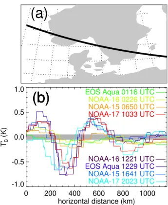
while maintaining the same wavelength and phase out to 12:29 UTC. The wavelength along this trajectory is∼400– 500 km, with slight increases by 16:41 UTC and 20:23 UTC. 5.2 NWP model fields

To isolate gravity wave perturbations from temperature fields generated by any one of our three NWP models, we use al-gorithms similar to those just described and applied to the AMSU-A radiances. First, the three-dimensional tempera-ture fields at a given model time were regridded vertically from their terrain-following model coordinates to a common high-resolution set of constant pressure surfaces to yield a 3-D temperature fieldT (λ,ˆ φ, p)ˆ , where p is pressure. A background temperature field T (¯ λ,ˆ φ, p)ˆ was computed at each pressure level using a two-dimensional running aver-age with a width of∼600–650 km. The precise width of this averaging window varied slightly from model to model, due to the different horizontal gridpoint resolutions1hand the resulting integer number of gridpointsnneeded to yield an averaging windown1hwithin this 600–650 km range.

Perturbations were derived as

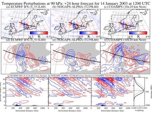
T′(λ,ˆ φ, p)ˆ =T (λ,ˆ φ, p)ˆ − ¯T (λ,ˆ φ, p).ˆ (4) The upper two rows of Fig. 8 plot T′(λ,ˆ φ, p)ˆ fields at p=90 hPa from the three NWP models for +24 h fore-casts initialized on 13 January 2003 at 12:00 UTC, valid at 12:00 UTC on 14 January. They show a mountain wave oscil-lation over southern Scandinavia with a geographical extent and phase structure very similar to the 12:00 UTC AMSU-A brightness temperature perturbations in Figs. 6e and f.

The bottom panels in Fig. 8 plot altitude cross sections of the temperature fields along the horizontal line plotted as the black curve in the panels above, which is the same trajectory used in Fig. 7a. Each NWP model produces a similar-looking mountain wave temperature oscillation that grows in ampli-tude with altiampli-tude up to 10 hPa and beyond. The horizontal wavelengthλh is∼400–500 km and the vertical wavelength λzis∼12 km. The vertical range of the AMSU-A Channel 9

radiance acquisition through this wave structure is depicted in Fig. 8j using the 1-D vertical weighting functions for the near-nadir and far off-nadir scan angles from Fig. 1b.

The most obvious difference among the three model fields is in the wave amplitudes. At 90 hPa, NOGAPS-ALPHA yields peak amplitudesTPEAK ∼4.5 K, ECMWF IFS yields

TPEAK∼6 K, and COAMPS yieldsTPEAK∼7 K. This increas-ing trend in wave amplitudes is consistent with increases in horizontal and vertical model resolution. Since the very smallest resolved scales in NWP models have little predictive skill (Lander and Hoskins, 1997; Davies and Brown, 2001), NWP models smooth their gridscale orography (Derber et al., 1998; Webster et al., 2003) and apply scale-selective numer-ical damping to their prognostic fields (Skamarock, 2004) to suppress these smallest scales. As a result, only at hori-zontal wavelengths greater than∼6–10 times the minimum

0 200 400 600 800 1000

horizontal distance (km) -1.0

-0.5 0.0 0.5 1.0

T’B

(K)

EOS Aqua 1229 UTC

(b)

(b)

NOAA-15 1641 UTC

(b)

NOAA-15 0650 UTC

(b)

NOAA-16 1221 UTC

(b)

(b)

NOAA-17 2023 UTC

(b)

NOAA-17 1033 UTC

(b)

(a)

Fig. 7. Panel(b) plots AMSU-A brightness temperature pertur-bations along the horizontal trajectory plotted in (a), for all 8 overpasses plotted in Fig. 6. Gray strip in (b) marks the range

±0.16/3 K, the nominal noise-limited detection threshold after 3×3 point smoothing (Lambrigtsen, 2003).

horizontal gridpoint resolution1hdo waves appear in these models without significant attenuation of their amplitudes (Davies and Brown, 2001; Skamarock, 2004). Vertical reso-lution differences in Fig. 1a also contribute, though previous studies suggest they are secondary to horizontal resolution for gravity waves in the extratropics so long as the vertical wavelength is sufficiently long (e.g., O’Sullivan and Dunker-ton, 1995; Hamilton et al., 1999).

Previous studies of Scandinavian stratospheric mountain waves in global and mesoscale models have shown that the resolved wave amplitudes in the global model can be un-derestimated by anywhere up to 50–80%. Hertzog et al. (2002) analyzed a stratospheric mountain wave over south-ern Scandinavia with a much shorter horizontal wavelength than here (λh∼200 km) and a slightly shorter vertical

wave-length (λz∼10 km). While the estimated wave amplitude

at ∼20 hPa was ∼9 K, the wave resolved in the ECMWF IFS TL319L60 analyses had an amplitude of only 1.5 K and the horizontal wavelength was overestimated. TL319 corresponds to 1hof ∼60 km on the N160 reduced linear Gaussian grid. Since thisλh∼200 km wave spans only 3–

(a) ECMWF IFS (TL511L60)

-6.3 K 6.3

(d) ECMWF IFS (TL511L60)

-4-3-2 -1 -1 1 1 1 2 2 34

0 200 400 600 800 1000

horizontal distance (km) 0 5 10 15 20 25 30

pressure height (km)

(g) ECMWF IFS (TL511L60) Cross Section

-4 -2 -2 -2 -2 0 0 0 0 0 0 0 ₀ 2 2 2 2 2 4 4 4

(b) NOGAPS-ALPHA (T239L60)

-4.5 K 4.5

(e) NOGAPS-ALPHA (T239L60)

-3 -2 -1 -1 1 1 1 1 1 2 2 3

0 200 400 600 800 1000

horizontal distance (km) (h) NOGAPS-ALPHA (T239L60) Cross Section

-2 -2 -2 -2 -2 0 0 0 0 0 0 0 0 0 0 2 2 2 2 4 4 6

(c) COAMPS (10x10 km Nest)

-6.9 K 6.9

(f) COAMPS (10x10 km Nest)

-4 -2 -2 -2 -1 -1 -1 -1 1 1 1 1 1 1 1 2 2 2 2 2 4 4 4 6

0 200 400 600 800 1000

horizontal distance (km) (i) COAMPS (10x10 km Nest) Cross Section

-10

-8 -8

-6

-6 -4 -4

-4 -4 -4 -4 -4 -2 -2 -2 -2 -2 -2 -2 _-2

0 0 0

0 0 0 0 0 0 0 0

0 ₀ 0

2 2 2 2 2 2 2 2 4 4 4 4 4 6 6 6 8 8 1012

Temperature Perturbations at 90 hPa: +24 hour forecast for 14 January 2003 at 1200 UTC

(j)

0.000 0.025 0.050 weighting

1000 100 10

pressure (hPa)

Fig. 8. Top row plots temperature perturbationsT′(λ,ˆ φ, p)ˆ atp=90 hPa extracted from +24 h forecasts from ECMWF IFS (left column), NOGAPS-ALPHA (middle column) and COAMPS (right column) runs, using a similar map range to AMSU-A brightness temperature perturbations in Fig. 6. See color bar in the lower-right corner of each panel for temperature range. Middle row plots same fields, but now focused over southern Scandinavia. Contour interval is 1 K. Bottom row of plots shows altitude contours ofT′(λ, φ, p)along the horizontal cross section plotted as black curve in the panels above. Negative (cold) temperature anomalies are blue, positive (warm) temperature anomalies are red, and the contour interval is 2 K (zero contour is omitted). Cross sections of topographic surface elevations are shaded in gray. Panel(j)replots AMSU-A Channel 9 1-D vertical weighting functions from Fig. 1b.

A mountain wave with wavelengths closer to the current example occurred over northern Scandinavia on 26 January 2000: NWP forecasts yieldedλh∼400 km, λz∼10 km and TPEAK∼9 K at 30 hPa (D¨ornbrack et al., 2002; Fueglistaler et al., 2003; Eckermann et al., 2006). Eckermann et al. (2006) found that the wave temperature amplitude in the TL319L60 ECMWF IFS forecast fields was 50% lower than in a mesoscale model run (see also Fueglistaler et al., 2003). In this case, the horizontal wavelength λh∼400 km spans

around 6–7 ECMWF gridpoints, bringing it into the 61h– 101h transition zone where Skamarock (2004) found that dynamics were resolved but somewhat suppressed in energy. Our λh∼400–500 km mountain wave in the 1h=10 km

nested COAMPS run spans 40–50 horizontal gridpoints. Ac-cording to Skamarock (2004), COAMPS should accurately simulate this wave, and thus for now we will take its sim-ulated wave amplitude to represent the true wave ampli-tude. The TL511 ECMWF spectral resolution corresponds to

1h∼40 km on the reduced N256 linear Gaussian grid, mak-ing ourλh∼400–500 km wave a 101hoscillation in these

fields and placing it at the high end of the 6–101h transi-tion zone where amplitudes are not greatly suppressed (Ska-marock, 2004). A comparison of Figs. 8a and c bears this out. NOGAPS-ALPHA’s T239 spectral resolution yields a gridpoint resolution on the 720×360 quadratic Gaussian grid

of∼55 km at the equator, though the intrinsic resolution to zonal wavelengths is nearer 80 km at the equator. This places our wave in NOGAPS-ALPHA fields somewhere in the 5– 91hrange where we expect some significant amplitude un-derestimatation (Skamarock, 2004; Eckermann et al., 2006), consistent with amplitude differences between Figs. 8a and c.

5.3 Suborbital validation of NWP model fields

For a more direct and objective assessment of the fidelity of the gravity waves in these NWP fields, we now compare them directly to suborbital measurements of the lower stratosphere over southern Scandinavia on 14 January 2003.

5.3.1 Radiosonde

amplitudes evident in the NWP model fields in Fig. 8. As-suming an ontime 12:00 UTC launch, we estimate the bal-loon reached 90 hPa just before 13:00 UTC.

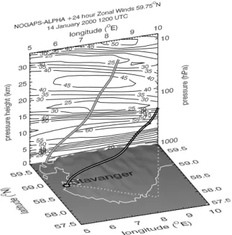
The contours in Fig. 9 show the NOGAPS-ALPHA +24 h (12:00 UTC) zonal winds at 59.75◦N. They reveal strong surface westerlies of ∼20 m s−1 that increase with height to a tropopause jet stream exceeding 60 m s−1, and a wave-induced horizontal velocity oscillation of around±10 m s−1 in the stratosphere superimposed on mean westerlies of 30– 40 m s−1. The strong westerly flow at all altitudes is consis-tent with surface forcing of quasi-stationary mountain waves and free propagation of those waves into the stratosphere (i.e., no critical level). The wave phase lines slope downward on progressing eastward, as in the temperature cross sec-tions in Figs. 8g–i, consistent with a quasi-stationary moun-tain wave propagating upward and westward in this eastward flow.

Observational studies often assume that gravity wave fluc-tuations in radiosonde data can be interpreted as a purely vertical profile through the 3-D wave field directly above the launch site. Here, however, the strong westerlies ad-vect the balloon substantial distances to the east. Figure 9 shows rather clearly in this case that the radiosonde samples a significantly different wave structure along its oblique as-cent trajectory than the purely vertical profile directly above Stavanger, an issue highlighted in some previous observa-tional studies of mountain waves using radiosonde data (e.g., Shutts et al., 1988; Lane et al., 2000). Thus our model-data comparison in Fig. 10 compares the radiosonde zonal winds

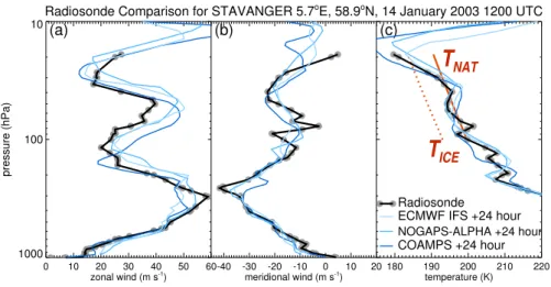
U, meridional windsV and temperaturesT with correspond-ing 12:00 UTC fields from the 3 NWP model runs that were sampled along the 3-D radiosonde trajectory in Fig. 9.

The NWP wind and temperature profiles in Fig. 10 are close to the radiosonde data at all altitudes. The stratospheric wave oscillation is most prominent in the zonal winds in Fig. 10a. The model fields reproduce its amplitude and phase quite well, given the uncertainties in the actual balloon trajec-tory, model errors and slight time mismatches between NWP fields and the radiosonde. Though the wave appears more weakly in the meridional wind and temperature profiles, the NWP fields match the amplitude and phase structure well in these profiles too.

The upper-level radiosonde temperatures in Fig. 10c are extremely cold. The final radiosonde measurement of 179.6 K near 19 hPa is only∼1 K warmer than the record low stratospheric radiosonde temperature of 178.6 K reported by D¨ornbrack et al. (1999) from 35 years of soundings from So-dankyl¨a (67.4◦N, 26.7◦E) in northern Finland (though this record value was subsequently eclipsed in January 2001: see Kivi et al., 2001). Since Stavanger/Sola lies some 8.5◦ equa-torward of Sodankyl¨a, this low temperature is unusual and or-dinarily might be questioned given that it was the final mea-surement acquired just prior to the balloon bursting. How-ever, the NWP model profiles computed along its ascent tra-jectory in Fig. 10c strongly suggest that the data here are

Fig. 9. Solid black curve with white stripe shows the estimated 3-D trajectory of the radiosonde launched from Stavanger on 14 January 2003 at 12:00 UTC. Shaded 3-D surface shows topographic elevations from the ETOPO5 database. Contours show zonal winds in m s−1(positive values are eastward) at 59.75◦N from the +24 h NOGAPS-ALPHA hindcast. The latitude-height projection of the 3-D radiosonde trajectory is plotted in gray with white stripe.

reliable, and that these cold temperatures result from passage of the balloon through the cooling phase of a large-amplitude stratospheric mountain wave.

5.3.2 NASA DC-8 flight

Red curves in Fig. 10c show that these very cold tempera-tures at 20 hPa lie below the frost point temperatureTICE, which should cause type II (ice) PSCs to form here if nucle-ation material is present. Aerosol lidar data acquired from a NASA DC-8 flight on this day allow us to test this inference, and to validate the NWP model fields further.

During January 2003 the DC-8 was operating from Kiruna airport (67.8◦N, 20.3◦E) in northern Sweden, in support of NASA’s second SAGE III Ozone Loss and Validation Exper-iment (SOLVE II; see McCormack et al., 2004). The cold synoptic stratospheric conditions and stratospheric mountain wave activity over southern Scandinavia on 14 January 2003 were both forecast several days beforehand using ECMWF IFS fields and the NRL Mountain Wave Forecast Model (MWFM), extending similar in-field wave forecasting efforts inaugurated for SOLVE during 1999–2000 and reported by Eckermann et al. (2006).

0 10 20 30 40 50 60

zonal wind (m s-1₎

1000 100 10

pressure (hPa)

(a)

-40 -30 -20 -10 0 10 20

meridional wind (m s-1₎

(b)

180 190 200 210 220

temperature (K) (c)

Radiosonde Comparison for STAVANGER 5.7o_{E, 58.9}o_{N, 14 January 2003 1200 UTC}

Radiosonde

COAMPS +24 hour NOGAPS-ALPHA +24 hour ECMWF IFS +24 hour

T

T

Fig. 10. Gray circles connected by solid black curve show data acquired from the 14 January 2003 12:00 UTC radiosonde sounding from Stavanger: (a)zonal winds;(b)meridional winds; (c)temperatures. Blue curves show output from the +24 h ECMWF IFS operational forecast, the +24 h NOGAPS-ALPHA hindcast, and the +24 h COAMPS hindcast, all valid for 12:00 UTC on 14 January 2003, computed along the 3-D radiosonde trajectory in Fig. 9. Red curves in (c) show nominal threshold temperaturesTICEandTNATfor formation of ice

and nitric acid trihydrate, respectively, assuming typical stratospheric values of 5 ppmv of water vapor and 10 ppbv of nitric acid (Hanson and Mauersberger, 1988; Marti and Mauersberger, 1993).

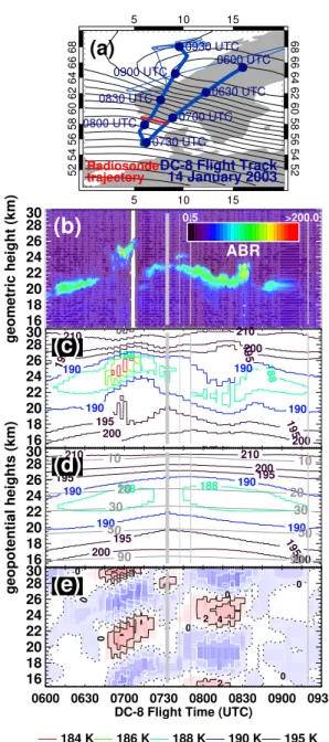
rapidly eastward across central Scandinavia, bringing with it strong surface westerly flow across the southern Scandi-navian Mountains. The near-zero surface winds over central Scandinavia in the core of the low and weak surface easterlies across northern Scandinavia account for the confinement of the stratospheric wave activity to the south, since little moun-tain wave activity is forced over central Scandinavia, while any waves generated to the north are absorbed at upper tro-pospheric critical levels as the flow transitions from surface easterlies to upper tropospheric and stratospheric westerlies. The SOLVE II forecasts for 14 January predicted PSCs forming within the cold phases of mountain waves over southern Scandinavia. Based on this forecast guidance, a DC-8 flight from Kiruna was devised containing a south-ward leg to fly beneath these forecast wave PSCs and pro-file them with onboard lidars. The final DC-8 flight track is plotted in blue in Fig. 11a, with filled circles marking ev-ery 30 min along the flight segment from 06:00–09:30 UTC. The radiosonde trajectory from Fig. 9 is plotted in red. We see that the DC-8 flew beneath the cold 20 hPa stratospheric region sampled at the end of the radiosonde trajectory just after 07:00 UTC, some 5–6 h before the radiosonde sampled this region. From the AMSU-A data in Fig. 6c, the moun-tain wave appeared to be present in this region at 07:00 UTC when the DC-8 arrived, but had a weaker amplitude than at the time of the radiosonde intercept at 12:00–13:00 UTC.

Figure 11b plotsS1064from the GSFC/LaRC lidar returns (see Sect. 2.2) from 06:00 UTC to 09:30 UTC, a flight seg-ment marked with the thicker blue line in Fig. 11a. Extensive PSC aerosol was measured in a number of thin tilted layers in the 20–26 km altitude range. Isolated yellow–red regions

whereS1064is∼50–200 likely indicate ice (type II) PSCs. Figure 11c plots temperatures T (λ,ˆ φ, Zˆ geo) from the NOGAPS-ALPHA +19 h hindcast (valid at 07:00 UTC) along this DC-8 flight track. Here we have profiled the fields as a function of model geopotential heightZgeo rather than pressure heightZ, to permit more direct comparison with the geometric altitude registration of the lidar data. The coldest temperature contours≤190 K are color coded, and correlate impressively in altitude and variation with flight time with the lidar data in the panel above. In particular the isolated re-gion of largeS1064at 25 km at 07:00 UTC is colocated with a compact region of the coldest NOGAPS-ALPHA tempera-tures of∼184 K, plotted as red contours. This 25 km altitude corresponds to pressures of∼18–20 hPa (see grey contours in Fig. 11d). From Fig. 11a we see that this isolated type II PSC layer measured at 07:00 UTC in panel (b) occurs at the same geographical location intercepted 5–6 h later by the ra-diosonde, which measured very cold temperaturesT <TICE in Fig. 10c that should form ice PSCs. Thus the radiosonde, lidar and NWP temperature data all cross-validate at this lo-cation.

5 10 15

5 10 15

52 54 56 58 60 62 64 66 68 52 54 56 58 60 62 64 66 68 0600 UTC 0630 UTC 0700 UTC 0730 UTC 0800 UTC 0830 UTC 0900 UTC 0930 UTC

(a)

DC-8 Flight Track 14 January 2003

Radiosonde trajectory 16 18 20 22 24 26 28 30

geometric height (km)

0.5 >_200.0

ABR

(b)

(c)

geopotential heights (km)

188 188 190 190 190 190 195 195 195 195 200 200 200 200

210 ₁₀ 210 ₁₀

20 20 30 30 50 50 90 90

(d)

0600 0630 0700 0730 0800 0830 0900 0930 DC-8 Flight Time (UTC)

16 18 20 22 24 26 28 30 -2 -2 0 0 0 0 0 0 0 2 2 4

(e)

184 K 186 K 188 K 190 K 195 K

Fig. 11. (a)Blue curves show DC-8 flight of 14 January 2003, with period from 06:00–09:30 UTC highlighted with thicker curve and 30 min markers. Red curve shows horizontal radiosonde tra-jectory from Fig. 9. Contours show 12:00 UTC 925 hPa NAVDAS analyzed geopotential heights.(b)S₁₀₆₄from GSFC/LaRC aerosol lidar from 06:00–09:30 UTC, derived as 8 point averages of the raw data (4 points in time, 2 points in height). Gray strips omit data where DC-8 turned in (a) to roll angles>5◦which tilted the lidar beam off zenith. Color bar scale is logarithmic. (c)Temperatures

T along DC-8 flight track from NOGAPS-ALPHA +19 h forecast, valid at 07:00 UTC, plotted versus model geopotential height. Con-tour color scale is shown beneath panel(e). (d)as for (c) but plot-ting mean temperaturesT¯. Gray contours show pressure surfaces in hPa. (e) as for (c) but plotting temperature perturbationsT′, the dif-ference field between (c) and (d). Contour interval is 2 K, positive values are red and negative values are blue.

180 185 190 195 200 205 210

temperature (K)

16

18

20

22

24

26

28

altitude (km)

AROTAL

Temperatures above DC-8: 0649-0654 UTC

(59.86

N, 9.91

E)

ECMWF IFS

NOGAPS-ALPHA

Fig. 12. Black curves show raw AROTAL Rayleigh temperatures acquired from the DC-8 on 14 January from 06:49–06:54 UTC. Blue curves show temperature profiles at the closest horizontal gridpoint to this flight segment from the NOGAPS-ALPHA +19 h hindcast (valid at 07:00 UTC) and the ECMWF IFS +18 h forecast (valid at 06:00 UTC). Gray strip shows estimated altitudes where the AROTAL temperature retrieval is significantly contaminated by PSC aerosol layers.

layers were observed earlier in the flight in Fig. 11b, and thus contain aerosol which can contaminate the retrieval. Indeed, the cold temperature “biteout” in the data at 21 km in Fig. 12 resembles the structure of the PSC-contaminated retrieved Rayleigh temperature profile shown in Fig. 7 of Burris et al. (2002b). Thus we view AROTAL temperatures in this region as suspect. Above this grey strip (Z≥23 km), we assume more PSC-free air that yields a more accurate retrieved tem-perature. Specifically, at 25 km the AROTAL temperatures drop to a minimum of∼184 K, which again agrees well with the NOGAPS-ALPHA temperatures in Figs. 11c and 12 and is consistent with the ice PSC encountered minutes later at this altitude by the DC-8.

16 18 20 22 24 26 28 30

188 188

190

190

195

195

195

195

200

200

200

(a)

178 K 180 K 182 K 184 K 186 K 188 K

geopotential heights (km)

0600 0630 0700 0730 0800 0830 0900 0930 DC-8 Flight Time (UTC)

16 18 20 22 24 26 28 30

188

190

195 195

195

195

200 200

200

200

210 210

(b)

Fig. 13. Same presentation as in Fig. 11c, but profiling temper-atures from(a)COAMPS +19 h hindcast, valid at 07:00 UTC, and (b)NOGAPS-ALPHA +24 h hindcast, valid at 12:00 UTC. Contour color scale is shown above panel (a).

else. Clearly the omitted wave component produces most of the observed structure in these PSC layers. The perturbation temperatures in Fig. 11e show that the ice PSC at 07:00 UTC is produced by a mountain wave-induced temperature per-turbation that cools this region by about 6–8 K. This then is clearly a mountain wave–induced ice PSC.

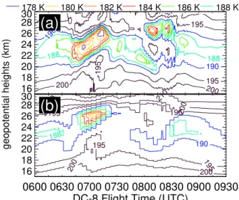
The minimum NOGAPS-ALPHA temperature in Figs. 11c and 12 of∼184 K is at or just slightly above the 20 hPa frost point temperature shown in red in Fig. 10c. That ice PSCs were measured here suggests that wave amplitudes were underestimated in the NOGAPS-ALPHA run, consistent with our earlier inferences based on its T239L60 resolution. To assess this, Fig. 13a plots corre-sponding 07:00 UTC temperatures from the COAMPS run, which show a thicker layer of much colder temperatures at 07:00 UTC due to larger wave amplitudes in this higher resolution model.

At 12:00–13:00 UTC when the radiosonde entered this re-gion, the minimum 12:00 UTC NOGAPS-ALPHA tempera-ture along the radiosonde trajectory in Fig. 10c was∼180 K, significantly colder than the 184 K in Fig. 11c. This sug-gests that the wave in the NOGAPS-ALPHA run grew sig-nificantly in amplitude from 07:00 UTC to 12:00 UTC, con-sistent with what the AMSU-A data in Fig. 6 appear to show. To assess this, Fig. 13b plots corresponding NOGAPS-ALPHA temperatures along the DC-8 flight trajectory using the +24 h forecast fields, valid at 12:00 UTC. We see that the minimum temperatures are now 180 K, 4 K cooler than in Fig. 11c, indicating a growth in peak wave amplitude of

∼4 K from 07:00 UTC to 12:00 UTC, and again consistent with the 179.2 K radiosonde temperature measured at 19 hPa in Fig. 10c.

6 Brightness temperature perturbations from forward

modeled NWP temperature fields

Having validated the NWP temperature fields against avail-able suborbital data, we now insert these fields into Eq. (2) to derive anticipated AMSU-A Channel 9 brightness temper-ature perturbations, which we compare against the observed AMSU-A perturbations. This represents our approach to val-idating the gravity wave signals in AMSU-A Channel 9 radi-ances.

6.1 Forward modeled NWP temperature perturbations We begin with direct forward modeling of the NWP wave temperature perturbation fieldsT′(λ,ˆ φ, p)ˆ to yield a bright-ness temperature perturbation field

T_B′

NWP(Xj, Yj)= Z Z Z

Wj(X−Xj, Y −Yj, Z)

T′(X, Y, Z)dXdY dZ. (5) Similar calculations for idealized 3-D wave temperature os-cillations were performed by Eckermann and Wu (2006).

To facilitate direct comparisons with AMSU-A imagery, here we use the orbital scan geolocations from each AMSU-A overpass to synthesize forward-modeled swath-scanned pushbroom images, using the algorithms outlined in Sect. 3.2 and the NWPT′(λ,ˆ φ, p)ˆ field closest in time to each over-pass. FinalT_B′

NWP(λˆj,φˆj)maps incorporated the same 3×3 point smoothing applied to the AMSU-A perturbations in Fig. 6. Figure 14 plots resulting T_B′

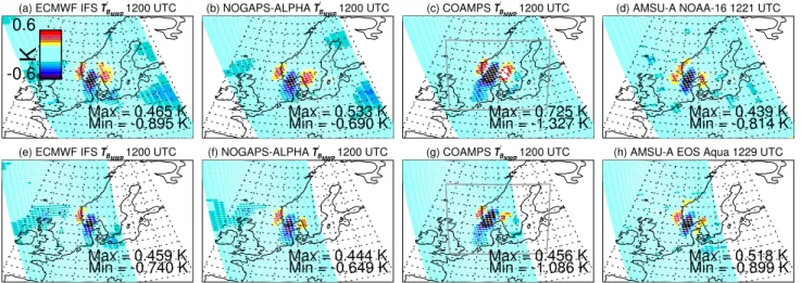
NWP(λˆj,φˆj)fields for AMSU-A 12:21 UTC measurements from NOAA-16 (top row) and 12:29 UTC measurements from EOS Aqua (bottom row), based on 12:00 UTC (+24 h forecast)T′(λ,ˆ φ, p)ˆ fields from ECMWF IFS, NOGAPS-ALPHA and COAMPS. The corresponding AMSU-A data from Fig. 6 are reproduced in the right panels of Fig. 14 for comparison.

The synthetic NWP T_B′ NWP(

ˆ

λj,φˆj) maps all show a

wave oscillation over southern Scandinavia that matches the AMSU-A data well in location, horizontal extent, orienta-tion and phase. In terms of amplitude, the ECMWF IFS amplitudes are close to the measured values. The NOGAPS-ALPHA amplitudes are smaller, consistent with expected un-derprediction of wave amplitudes in these T239L60 runs, as discussed in Sect. 5.2. The COAMPS amplitudes are fairly close to the EOS Aqua AMSU-A observations, but somewhat larger than the NOAA-16 AMSU-A observations.

Indeed, despite using the same 12:00 UTC T′(λ,ˆ φ, p)ˆ

fields, all the resultingT_B′

(a) ECMWF IFS T’

BNWP1200 UTC

Min = -0.895 K Max = 0.465 K

(e) ECMWF IFS T’

B_NWP1200 UTC

Min = -0.740 K Max = 0.459 K

(b) NOGAPS-ALPHA T’

BNWP1200 UTC

Min = -0.690 K Max = 0.533 K

(f) NOGAPS-ALPHA T’

B_NWP1200 UTC

Min = -0.649 K Max = 0.444 K

(c) COAMPS T’

BNWP1200 UTC

Min = -1.327 K Max = 0.725 K

(g) COAMPS T’

B_NWP1200 UTC

Min = -1.086 K Max = 0.456 K

(d) AMSU-A NOAA-16 1221 UTC

Min = -0.814 K Max = 0.439 K

(h) AMSU-A EOS Aqua 1229 UTC

Min = -0.899 K Max = 0.518 K

-0.6 0.6

K

Fig. 14. Top row shows brightness temperature perturbationsT_B′ NWP(

ˆ

λj,φˆj)computed from Eq. (5) using 12:00 UTC NWP temperature perturbation fieldsT′(λ,ˆ φ, p)ˆ from(a)ECMWF IFS,(b)NOGAPS-ALPHA, and(c)COAMPS runs using AMSU-A scan pattern from the NOAA-16 12:21 UTC overpass. Actual brightness temperatures extracted from these AMSU-A measurements are replotted in(d)from Fig. 6e. Bottom row shows same sequence of plots for the 12:29 UTC EOS Aqua overpass data. Gray borders in (c) and(g)show the regional COAMPS domain. Color bar scale (±0.6 K) is given at the top-left of panel (a). Maximum and minimum values for each map are shown in the lower-right portion of each panel.

The smaller EOS Aqua T_B′

NWP(λˆj,φˆj) amplitudes in Fig. 14 arise due to the height variation of the wave tem-perature amplitudes in the NWP models. As shown in the bottom row of Fig. 8, the wave temperature amplitudes in all 3 models decrease between 80–90 hPa and 50–60 hPa. For example, the corresponding maximum ECMWF IFS ampli-tude at 60 hPa is 4.8 K compared to the 6.3 K at 90 hPa in Fig. 8a. The wave in the NOAA-16 12:21 UTC overpass data lies near the center of the scan pattern and so is ob-served by the near-nadir beams whose weighting functions peak near 80–90 hPa. Conversely, the wave is located to-wards the right edge of the EOS Aqua scan pattern, where it is observed by off-nadir beams which peak at higher al-titudes (see Fig. 8j). The weaker NWP model temperature amplitudes at these higher altitudes lead to a weaker NWP brightness temperature perturbation for the EOS Aqua scan. In contrast to the model fields, the observed AMSU-A per-turbation amplitudes are slightly larger for the EOS Aqua overpass in Fig. 14h than for the NOAA-16 overpass in Fig. 14d. This suggests that, while the NWP models have captured the wave structure and mean wave amplitudes quite well, the actual vertical variation in wave amplitudes over the 50–90 hPa range may have differed from the model predic-tions.

6.2 Perturbations isolated from forward modeled NWP temperatures

Next we perform more realistic forward modeling by using the raw NWP model temperature fields to simulate a

bright-ness temperature field TBNWP(λˆj,φˆj) using Eq. (2), as in Fig. 2. Then, we apply exactly the same data reduction algo-rithms to these brightness temperature fields that we applied to the AMSU-A brightness temperature data in Sect. 5.1, first deriving a background fieldT¯BNWP(λˆj,φˆj)and then, follow-ing Eq. (3), computfollow-ing perturbation fields

T_B′

NWP(λˆj,φˆj)=TBNWP(λˆj,φˆj)− ¯TBNWP(λˆj,φˆj). (6) Finally, 3×3 point smoothing is applied to these perturbation fields. Differences between perturbation fields calculated us-ing this method and those calculated in Sect. 6.1 provide some feel for how well the numerical data reduction meth-ods in Sect. 5.1 isolate gravity wave perturbations from raw AMSU-A radiances.

Figure 15 plots NWP perturbation brightness temperatures calculated using this method for the same set of 12:00 UTC fields and AMSU-A scans shown in Fig. 14. Oscillatory structure that closely resembles the measurements (panels d and h) is reproduced in all the NWP-based radiance fields over southern Scandinavia. On comparing with correspond-ing panels in Fig. 14, we see thatT_B′

(a) ECMWF IFS T’

BNWP1200 UTC

Min = -0.686 K Max = 0.504 K

(e) ECMWF IFS T’

BNWP1200 UTC

Min = -0.604 K Max = 0.440 K

(b) NOGAPS-ALPHA T’

BNWP1200 UTC

Min = -0.484 K Max = 0.448 K

(f) NOGAPS-ALPHA T’

BNWP1200 UTC

Min = -0.488 K Max = 0.436 K

(c) COAMPS T’

BNWP1200 UTC

Min = -1.116 K Max = 0.669 K

(g) COAMPS T’

BNWP1200 UTC

Min = -0.922 K Max = 0.505 K

(d) AMSU-A NOAA-16 1221 UTC

Min = -0.814 K Max = 0.439 K

(h) AMSU-A EOS Aqua 1229 UTC

Min = -0.899 K Max = 0.518 K -0.6

0.6

K

Fig. 15.Same presentation as Fig. 14, but now plotting NWP brightness temperature perturbations derived by extracting them from mean values via Eq. (6).

Figure 16 plotsT_B′

NWP(λˆj,φˆj)maps based on NOGAPS-ALPHA temperature fields at times closest to the correspond-ing measurements from all 8 AMSU-A overpasses in Fig. 6. Many aspects of the measurements in Fig. 6 are reproduced in Fig. 16. For example, at 01:00–02:00 UTC the pertur-bation maps look very similar despite showing no obvious wave perturbations over southern Scandinavia and small am-plitudes near nominal AMSU-A noise floors of∼0.15–0.2 K. At ∼07:00 UTC the wave appears weakly overly southern Scandinavia, then grows in amplitude during the period 07:00–12:00 UTC. The horizontal wavelength, geographical extent, orientation and phase all agree well with observed fluctuations in Fig. 6. At 17:00 UTC and 20:00 UTC the wave phase fronts are rotated clockwise compared to ear-lier times, the packet width is broader, the wavelength is longer, and the oscillation is dominated by a large-amplitude cold phase that extends farther northward and southward: all these features are seen in the observed maps in Figs. 6g and h. The main differences are in the amplitudes. For the first 6 panels, the NOGAPS-ALPHA brightness temper-ature amplitudes in Fig. 16 are smaller than those observed in Fig. 6. Whereas the largest observed perturbation ampli-tudes occur at∼12:00 UTC in Fig. 6, the largest NOGAPS-ALPHA brightness temperature amplitudes in Fig. 16 occur at 17:00 UTC and 20:00 UTC. This is due (at least in part) to the longer horizontal wavelength at these later times (see, e.g., Fig. 7b), which NOGAPS-ALPHA can explicitly simu-late at T239L60 with less amplitude attenuation (Skamarock, 2004).

Since the T239L60 NOGAPS-ALPHA runs underestimate this wave’s amplitude, we repeated these calculations using the hourly COAMPS fields. However, the regional COAMPS domain complicates these calculations. Specifically, when the numerical extraction methods used for AMSU-A data are applied to model brightness temperatures within this

re-gional COAMPS domain only, they produce edge effects at the lateral boundaries which severely contaminate the es-timated perturbation fields. To circumvent this issue, we generated artificial temperature fields at measurement loca-tions outside the COAMPS domain by averaging COAMPS temperatures that were within 200 km of the measurement point under consideration. If less than 50 COAMPS grid-points values were within 200 km of the measurement point, we averaged the 50 nearest gridpoint temperatures. We did this at each model level, then converted this artifical tempera-ture profile into a brightness temperatempera-ture by integrating verti-cally using the vertical AMSU-A weighting functionWj(Z).

Once a full map of brightness temperature data was gener-ated (both model-based fields inside and artificial fields out-side the COAMPS domain), we proceeded as before, com-puting means and then isolating fluctuations using Eq. (6).

Figure 17 plots these COAMPS-based T_B′

NWP(λˆj,φˆj) maps. The main differences from the NOGAPS-ALPHA fields in Fig. 16 are the larger amplitudes, as expected. These COAMPS fields agree quite well with AMSU-A data from the corresponding panels of Fig. 6. Overall, the largest COAMPS brightness temperature amplitudes are slightly larger than those observed in Fig. 6. Like the observations, the COAMPS fields return largest brightness temperature amplitudes at 12:00 UTC, with slightly smaller values at later times.

(a) NOGAPS-ALPHA T’

BNWP0100 UTC

Min = -0.189 K Max = 0.071 K

(b) NOGAPS-ALPHA T’

BNWP0200 UTC

Min = -0.220 K Max = 0.256 K

(c) NOGAPS-ALPHA T’

BNWP0700 UTC

Min = -0.284 K Max = 0.393 K

(d) NOGAPS-ALPHA T’

BNWP1000 UTC

Min = -0.409 K Max = 0.544 K

(e) NOGAPS-ALPHA T’

BNWP1200 UTC

Min = -0.484 K Max = 0.448 K

(f) NOGAPS-ALPHA T’

BNWP1200 UTC

Min = -0.488 K Max = 0.436 K

(g) NOGAPS-ALPHA T’

BNWP1700 UTC

Min = -0.642 K Max = 0.403 K

(h) NOGAPS-ALPHA T’

BNWP2000 UTC

Min = -0.688 K Max = 0.348 K -0.3

0.3

K

-0.6 0.6

K

Fig. 16.Similar presentation to Fig. 6, but showing brightness tem-perature perturbationsT_B′

NWP(

ˆ

λj,φˆj)derived via Eqs. (2) and (6) from the hourly NOGAPS-ALPHA temperature hindcast field clos-est in time to the satellite overpass in quclos-estion. Values are in Kelvin (see color bars): for panels(a)and(b)the range is±0.3 K, whereas for panels(c–h)the color bar range is±0.6 K. Maximum and min-imum values for each map are shown in the lower-right portion of each panel.

fields evident for the final 20:23 UTC NOAA-17 overpass. The close agreement between these model-generated and ob-served brightness temperature oscillations in Fig. 18 pro-vides an absolute validation of the gravity wave detection and imaging capabilities of AMSU-A Channel 9 radiances sug-gested by the modeling study of Eckermann and Wu (2006).

7 Summary and conclusions

This study has focused on structure in lower stratospheric radiances acquired from AMSU-A Channel 9 during 8 satel-lite overpasses of southern Scandinavia on 14 January 2003. On removing large-scale horizontal structure from the raw “pushbroom” radiance imagery, plane wave-like oscillatory structures were revealed over southern Scandinavia with horizontal wavelengths of∼400–500 km and amplitudes of

(a) COAMPS T’

BNWP0100 UTC

Min = -0.265 K Max = 0.263 K

(b) COAMPS T’

BNWP0200 UTC

Min = -0.276 K Max = 0.326 K

(c) COAMPS T’

BNWP0700 UTC

Min = -0.384 K Max = 0.305 K

(d) COAMPS T’

BNWP1000 UTC

Min = -0.842 K Max = 0.617 K

(e) COAMPS T’

BNWP1200 UTC

Min = -1.116 K Max = 0.669 K

(f) COAMPS T’

BNWP1200 UTC

Min = -0.922 K Max = 0.505 K

(g) COAMPS T’

BNWP1700 UTC

Min = -0.860 K Max = 0.381 K

(h) COAMPS T’

BNWP2000 UTC

Min = -0.926 K Max = 0.505 K -0.3

0.3

K

-0.6 0.6

K

Fig. 17. Same presentation as Fig. 16, but showing bright-ness temperature perturbationsT_B′

NWP(

ˆ

λj,φˆj)derived from hourly COAMPS temperature fields. Gray curve shows borders of the COAMPS domain. Black curves in panels(e–h)reproduce the cross section from Figs. 7a and 8 along which brightness temperatures are profiled in Fig. 18.

up to ∼0.9 K. Modeling studies by Eckermann and Wu (2006) indicated that long-wavelength large-amplitude grav-ity waves within the measurement volumes scanned by AMSU-A can produce this type of radiance structure. In such cases, this structure represents a quasi-horizontal measure-ment cross section through the 3-D gravity-wave oscillations near the 60–90 hPa peak in the Channel 9 weighting function. If validated, such measurements would provide an important new horizontal imaging capability for stratospheric gravity waves.