Adv. Sci. Res., 4, 63–69, 2010 www.adv-sci-res.net/4/63/2010/ doi:10.5194/asr-4-63-2010
©Author(s) 2010. CC Attribution 3.0 License.
Advances
in
Science & Research
Open Access ProceedingsEMS
Ann
ual
Meeting
and
9th
European
Conf
erence
on
Applications
of
Meteorology
2009
On the role of the planetary boundary layer depth
in the climate system
I. Esau1,2and S. Zilitinkevich1,3,4
1G.C. Rieber Climate Institute of the Nansen Environmental and Remote Sensing Center,
Thormohlensgt. 47, 5006, Bergen, Norway
2Bjerknes Centre for Climate Research, Bergen, Norway
3Division of Meteorological Research, Finnish Meteorological Institute, Helsinki, Finland
4Division of Atmospheric Sciences and Geophysics, Department of Physics, University of Helsinki, Finland
Received: 29 January 2010 – Revised: 13 April 2010 – Accepted: 26 April 2010 – Published: 17 May 2010
Abstract. The planetary boundary layer (PBL) is a part of the Earth’s atmosphere where turbulent fluxes dominate vertical mixing and constitute an important part of the energy balance. The PBL depth,h, is rec-ognized as an important parameter, which controls some features of the Earth’s climate and the atmospheric chemical composition. It is also known that hvaries by two orders of magnitude on diurnal and seasonal time scales. This brief note highlights effects of this variability on the atmospheric near-surface climate and chemical composition. We interpret heat capacity parameter of a Budyko-type energy balance model in terms of quasi-equilibriumh. The analysis shows that it is the shallowest, stably-stratified PBL with the smallesth
that should be of particular concern for climate modelling. The reciprocal dependence between the PBL depth and temperature (concentrations) is discussed. In particular, the analysis suggests that the climate characteris-tics during stably stratified PBL episodes should be significantly more sensitive to perturbations of the Earth’s energy balance as well as emission rates. On this platform,hfrom ERA-40 reanalysis data, the CHAMP satel-lite product and the DATABASE64 data were compared. DATABASE64 was used to assess the Troen-Mahrt method to determine hthrough available meteorological profile observations. As it has been found before, the shallow PBL requires better parameterization and better retrieval algorithms. The study demonstrated that ERA-40 and CHAMP data are biased toward deeperhin the shallow polar PBL. This, coupled with the scarcity of in-situ observations might mislead the attribution of the origins of the Arctic climate change mechanisms.
1 Introduction
The lowermost atmospheric layer where the vertical turbu-lent exchange is significant is known as the planetary bound-ary layer (PBL). The importance of the PBL for the Earth’s climate system has been recognized since pioneering work of Manabe and Strickler (1964). However, there are just a few studies (e.g. Knight et al., 2007), which excurse beyond the current narrow focus on PBL parameterizations in cli-mate models. Using a classification and regression tree ap-proach, Knight et al. (2007) demonstrated with 57 067 cli-mate model HadAM3 runs that 80% of variation in clicli-mate sensitivity to 2×CO2is associated with variation of a small
subset of parameters mostly related to the convection
pro-Correspondence to:I. Esau ([email protected])
64 I. Esau and S. Zilitinkevich: On the role of the planetary boundary layer depth in the climate system
et al., 2000; Byrkjedal et al., 2008). Nevertheless, at present, the primary attention of climatologists is still focused on the daytime PBL (Stone and Weaver, 2003; Walters et al., 2007). This study consists of two distinct sections. Section 2 looks at the bulk PBL effect and the PBL depth in a simple energy balance model. Section 3 addresses challenges of PBL depth diagnostics.
2 Bulk planetary boundary layer effect on the climate system
In spite of remarkable progress in climate modelling and ob-servation systems, a simple zero-dimensional energy balance climate model remains instrumental in understanding of the climate processes and mechanisms (North et al., 1981). In particular, utility of these models is in suggesting directions for statistical analysis of more comprehensive data from ob-servations and modelling in order to separate certain physical effects. Following (Budyko, 1969; North et al., 1981; Esau, 2008; Zilitinkevich and Esau, 2010), we consider a Budyko-type energy balance model. The model reads
CdT
dt ∝FT−FT0, (1)
whereT is temperature,FT is the divergence of the temper-ature flux, andC is the heat capacity of the system. On the Earth, positive and negative FT alternate on different time scales, primarily on diurnal and annual time scales, to make climate, i.e. the state where the averaged over many years
dT/dt→0. Addition of the averaged equilibrium flux,FT0,
for which dT/dt→0, allows studies of a transient climate
change in deviations from a unknown equilibrium state. Tra-ditionally, the attention of the climate research community is focused on investigation of perturbations caused by FT0
response on the shift of the radiation heat balance. North et al. (1981) review and the very recent Zaliapin and Ghil (2010) insightful analysis are just two examples of such a work. Contrary, the system heat capacity, C, has not re-ceived much attention. In a system where the role of tur-bulent mixing is significant, one can simplify asC∝h. Here,
we assumed that complexity of the turbulent mixing pro-cesses could be parameterized through a single integral pa-rameter, namely, the PBL depthh. The interested reader can find reservations and restrictions of this approach as well as supporting data in Esau (2008) and Zilitinkevich and Esau (2010).
As it follows from the traditional climatological conven-tion, T should be understood as the mean (global and sea-sonal averaged) surface air temperature. This convention im-mediately raises problems of aggregation of the system heat capacity and the temperature fluxes. We will not excurse into those problems making a silent assumption that both quanti-ties are aggregated properly. Moreover, we assume that our model in Eq. (1) does not have sub-scale temporal variabil-ity. The temperature change represents the direct transition
of the system from the unperturbed to a perturbed state. One should remember that these energy balance models are not to quantify behavior of the real Earth’s climate system, which is incomparably more complex, but to suggest approaches to data analysis.
Thus, with respect to the PBL effects, the model in Eq. (1) reads
dT dt =cT0
FT−FT0
h . (2)
Here,cT0is a non-dimensional proportionality coefficient,h
is dynamic quantity ultimately depending onFT0and
there-fore onT, which suggest a possible non-linear PBL feed-back in this kind of models. Esau (2008) and Zilitinkevich and Esau (2010) provided more materials to elaborate on the PBL feedback. We, however, will focus only on the bulk effects related to large variability ofh.
Equation (2) immediately reveals several falsifiable propo-sitions: (a) the temperature response to a given flux pertur-bation should have larger magnitude in the shallower PBL wherehis small; (b) the temperature variability should be larger in the shallow PBL; and (c) the temperature change is faster in the shallow PBL. One should observe that the temperature has probably stronger links with radiation pro-cesses and atmospheric large-scale dynamics hidden inFT0
than with the vertical turbulent mixing hidden inh. Manabe and Strikler (1964) and following works with the radiation-convective models (Ramanathan and Coakley, 1978; Randall et al., 1996) have demonstrated that this is not the case for the global scale climate as such. However, it could be the case for small perturbations (e.g. due to doubling of CO2 concen-tration) and on local scales. Moreover, only the local scale data will be available for direct analysis of the PBL effects as the nature of aggregation process remains unspecified.
One of possible ways to circumvent, at least partially, those difficulties is to recast Eq. (2) in terms of a scalar con-centration,Q. It reads
dQ dt =cQ0
FQ−FQ0
h , (3)
wherecQ0,cT0 is a non-dimensional proportionality
coef-ficient, Q is the scalar concentration and FQ0 is the
diver-gence of the scalar flux. IfQrepresents a long-lived scalar with its emission source predominantly within the PBL then, over sufficiently large homogeneous area,FQ0is mostly
con-trolled by the turbulent mixing. In this case, the bulk PBL effect could be separated in almost pure, laboratory condi-tions.
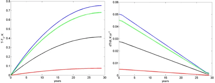
Figure 1. Response(a)of the temperature after Eq. (1) and its change rate(b)on an instant perturbation of the temperature flux by the observed green-house gas forcing. The constantcT0=1000 has been chosen in the way to bring the mean temperature change close to the observed one over the last 30 years. The black line denotes the mean temperature 0.5 (Tmax+Tmin); the blue line – the minimum temperature Tmin; the red line – the maximum temperatureTmax; the green line – the diurnal temperature range change (Tmin−Tmax). The initial state has been subtracted for all quantities.
– a characteristic depth of the convective, mostly daytime PBL; andhS∼O(102m) with the typical valuehS=150 m,
– a characteristic depth of the stably-stratified, mostly night-time PBL. These two distinct types of the PBL could be seg-regated in data and the corresponding temperature changes could be calculated. Since, in the most of cases, the turbu-lent convection is a dynamical reaction of the atmosphere on the positive surface heat balance, the convective PBL should be characterized by temperature maximums. Contrary, the stably stratified PBL forms during periods with the negative heat balance. Hence it should be characterized by tempera-ture minimums.
Several studies of the diurnal temperature maximum,Tmax,
and minimum,Tmin, have been published to date (e.g. Hansen
et al., 1995; Braganza et al., 2004; Vose et al., 2005). We consider here how the energy balance model in Eq. (2) will react on the gradual change of the forcing. The globally averaged green-house gas temperature forcing is ∆FT0∼
2.6×10⁻⁵K m s−1yr−1 for 30 year between 1979 and 2008
(Annual Greenhouse Gas Index, NOAA Earth System Re-search Laboratory, Global Monitoring Division, http://iasoa. org/iasoa/index.php). We impose a new climate equilibrium with FT1=FT0+30∆FT0 and integrate Eq. (2) to find the
minimum and maximum temperature adjustment in the deep and shallow PBLs correspondingly. To do this, we plot in Fig. 1 the following illustrative solution
T(t)−T(t=0)=cT0FT1 −FT(t)
h =cT0
30∆FT0−t∆FT0
h . (4)
As one can see,∆Tmaxincreases slower and changes on much
smaller value than∆Tmindoes. Therefore, the diurnal
tem-perature range (DTR) reduces. Its reduction accumulates
with time but the strongest reduction would be seen during periods of the strongest temperature flux forcing. Interesting that in warmer climate, it is rather unlikely to observe de-crease ofhCorhSsince the latter is already too small to show significant relative variations and the former cannot decrease in response on increasing temperature flux. There will be probably less cases and shorter periods withhS, which does not help to increase DTR either. Thus, the differential ex-treme temperature change and the decrease of the DTR over long time should be considered as the robust signature of the climate warming caused by the radiation balance shift due to the change of the atmospheric composition. In simple words, the difference in the PBL depth during day and night time leads to greatly suppressed response in the daytime tempera-ture relative to that in the night time.
Rudimentary and idealized estimations given above are however in surprisingly good agreement with available anal-ysis of observations. Braganza et al. (2004) give the rates ∆Tmax=0.1 K dec
−1
and ∆Tmin=0.2 K dec
−1
for the 50 years’ period between 1950 and 2000, which leads to (T−T0)max=0.3 K and (T−T0)min=0.6 K over 30 years.
However, Vose et al. (2005) and Hansen et al. (1995) found ∆Tmax≈∆Tmin≈0.29 K dec
−1
66 I. Esau and S. Zilitinkevich: On the role of the planetary boundary layer depth in the climate system
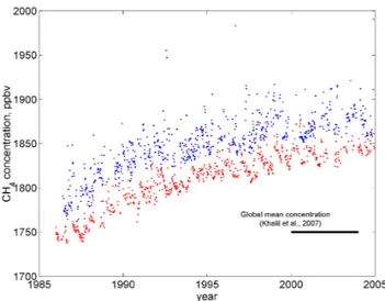
Figure 2. Daily averaged methane concentration obtained from NOAA/CMDL data at Barrow: red dots – summertime (June–July) data; blue dots – wintertime (December–January) data.
The differential temperature change is of primarily inter-est for climate research. The interinter-est in the concentration variability comes from many applications dealing also with shorter than decadal time scales. The bulk PBL effect on seasonal concentration of methane, CH4, is shown in Fig. 2.
This Figure reveals very powerful bulk PBL effect. The near surface concentration of CH4 is systematically higher
(by about 100 parts per billion in volume, ppbv) than the concentration of CH4 in the free atmosphere (Khalil et al.,
2007). This is expected as the primary CH4emission is
orig-inated from the surface (Walter et al., 2006). Since about 1998–1999, the average near-surface seasonal concentrations do not increase which is consistent with the global free at-mosphere records. Thus, one can conclude that the local emission of CH4 remains nearly constant over the period
of observations or it varies as a proportion of the free at-mosphere methane concentration, which is highly unlikely. Hence, both winter and summertime CH4concentrations are
determined by the local emission of the gas. Mastepanov et al. (2008) found significant methane release on the onset of the freezing season, which is a border between somewhat sig-nificant methane emission during the short polar summer (90 days or so) and much lower emission during the long polar winter (∼270 days). Despite lower emission rate in
winter-time, the CH4concentration remains significantly higher. It
exhibits large (∼50 ppbv) variations on a week scale, which
suggest that the individual release events could be mixed up into the free atmosphere during a week or so. At the same time, CH4 concentration always remains higher than that in
summertime. These facts can be explained with Eq. (3). Both larger CH4 concentration and larger variability are
under-stood as the effect of significant reduction of the PBL depth in response on the negative radiation balance and correspond-ing increase of the atmospheric stability. The convective
mo-tions are damped that both confines CH4in the shallow layer
ofhS∼100 m and prevents its exchange with the free
atmo-sphere due to build up of a strong radiation temperature in-version. ERA-40 (Uppala et al., 2005) data (a data selection within 2.5◦
by 2.5◦
rectangle centred at Barrow) revealed that
hC−hS is∼300 m. These data allow for rough estimation of the CH4 emission rate using only meteorological and
con-centration measurements. The mass of CH4 (per unit area),
MQ, emitted into the PBL should be equal to the mass of CH4
mixed into the free atmosphere during about 10 days. It can be calculated as
MQ= 1
2(Q−Q0)h. (5)
Now, we substitute for summertime Q=1820 ppbv, Q0=
1760 ppbv andhC=400 m. It gives the emission rateMQ∼ 1.2×10⁻⁵kg m−2day−1, which is fairly consistent with ∼
1.0×10⁻⁵kg m−2day−1 obtained by Walter et al. (2007) in
direct measurements. In wintertime, the numbers are as fol-lows, Q=1850 ppbv, Q0=1760 ppbv and hC=100 m. It gives the emission rateMQ∼4.5×10⁻⁷kg m−2day−1, which
is more than order of magnitude smaller than that in summer-time. Thus, shallower PBL in wintertime could maintain the higher CH4concentration in spite of the reduced emission.
3 Boundary layer depth diagnosis using observa-tions, models and satellite products
The PBL effects on climate are difficult to study becauseh
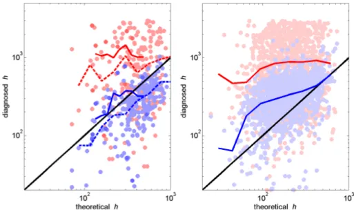
Figure 3.The daily averaged stably stratified quasi-steady state PBL depth,h. Days with convection and Monin-Obukhov length changes larger than∆L=50 m per day are excluded. Following Zilitinkevich et al. (2007), data were separated in(a)nocturnal (solid curves; light dots) and conventionally neutral (dashed curves; dark dots) PBLs;(b)long-lived stably stratified PBL. Bluish dots and blue curves are the ERA-40 data. Reddish dots and red curves are the CHAMP data. The curves are the bin-averaged values of the corresponding data.
the ERA-40 data are in good agreement with the present un-derstanding and turbulence-resolving simulation of the noc-turnal and near-neutral PBLs. Parameterizations for those layers have been thoroughly calibrated for the purpose of the mid-latitude weather prediction with the model. At the same time, the long lived stably stratified PBL remains a challenge for the model.
The over-prediction of the shallow PBL and the under-prediction of the deep PBL remain a challenging problem for other models as well. For instance Han et al. (2008) com-pared 5 PBL schemes in the Weather Research and Forecast-ing (WRF) model with observations in the Hong Kong area. Totally 145 samplings ofh were collected in 22 flights in March 2001. Both geographical and diurnal cycle patterns of
hshowed only moderate correlation (correlation coefficients vary from 0.65 to 0.7) to the observations. Typical noctur-nal biases were found to be of+300 m or about 100% of the observedhvalues. Typical daytime biases were found to be
−300 m or about 30% of the observedhvalues.
The diagnosis of the PBL depth in simulations (including ERA-40 reanalysis) and observations is usually based on the bulk Richardson number method by Troen and Mahrt (1986), which defines
h: Ri(z)=Ricr, where Ri= g θ0
θh−θs u2
h
z, (6)
θsis the surface potential temperature;θhis the potential tem-perature ath;uhis the wind speed ath;g/θ0=0.03 m s
−2
K−1
is the buoyancy parameter; andzis the height above surface. The method could be sensitive to a calibration of the criti-cal valueRicr. In meteorological practice, Ricr are taken in
the range from 0.15 to 1.0 with often quoted values of 0.25 and 0.5 (Serafin and Zardi, 2005; Jeriˇcevi´c and Grisogono, 2006). We investigated the variability ofhas function ofRicr
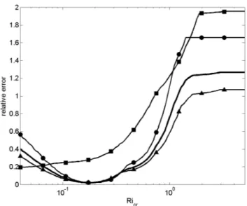
in the stably stratified PBL collected in the large-eddy sim-ulation database (The DATABASE64 could be downloaded from ftp://ftp.nersc.no/igor/NEW%20DATABASE64/; Esau and Zilitinkevich, 2006). Since the large-eddy simulations resolve the PBL turbulence, the DATABASE64 gives the op-portunity to determineh by different methods and to com-pare the results of directly determined PBL depth, i.e. us-ing turbulent flux profiles. Figure 4 shows the relative error, (hTM−hLES)/hLES, as a function ofRicr for the
convention-ally neutral, nocturnal stable and long-lived stable PBL av-eraged over all corresponding runs in DATABASE64. Here,
hTM is the PBL depth defined by Eq. (6), hLES is the PBL
depth defined as a level where the vertical momentum flux is equal to 5% of its surface value. The minimum error is found on average forRicrin the range 0.15 to 0.25.
Exclud-ing the nocturnal PBL, we conclude that the Troen–Mahrt method is robust with optimalRicr=0.2 and a negligible
68 I. Esau and S. Zilitinkevich: On the role of the planetary boundary layer depth in the climate system
Figure 4.The relative error (hTM−hLES)/hLES, as functions ofRicr
for the nocturnal stable (squares), conventionally neutral (circles) and long-lived stable (triangles) PBL averaged over all correspond-ing runs in DATABASE64. The bold line without symbols is the mean line for the later two types of the PBL.
4 Conclusions
This work is motivated by the fact that the planetary bound-ary layer depth, h, is important for the Earth’s climate. The first step to understand the bulk PBL effect on the Earth’s climate is to consider the energy-balance model. The model leads to reciprocal dependence between the temper-ature/concentration changes and h. The dependence can be summarized as: (a) the temperature response to a given flux perturbation has larger magnitude in the shallower PBL whereh is small; (b) the temperature variability should be larger in the shallow PBL; and (c) the temperature change is faster in the shallow PBL. These points were illustrated using the temperature response on the green-house gas forc-ing since 1979 and the seasonal variability of the methane concentration at point Barrow (Alaska, USA). We found reasonable agreement in the observed trends and variabil-ity between the methane concentrations, temperature anoma-lies and the PBL depth with numbers found in literature. We demonstrated that the model parameterizations (ERA-40) and the satellite products (CHAMP) over-predicthin shallow long-lived PBL typical in high-latitudes. This bias could and probably does cause climate model discrepancies in polar ar-eas as those reported by Beesly et al. (2000). This bias and the scarce in situ observations in the region makes it difficult to ascribe the polar climate change pattern.
Acknowledgements. The research leading to these results has received funding from the EC FP7/2007-2011 programme under grant agreement no. 212520, the EC ERC programme grant PBL-PMES and the Norwegian Research Council grant PBL-FEEDBACK.
Edited by: A. M. Sempreviva
Reviewed by: three anonymous referees
References
Beare, R. J., MacVean, M. K., Holtslag, A. A. M., Cuxart, J., Esau, I., Golaz, J.-C., Jimenez, M. A., Khairoutdinov, M., Kosovic, B., Lewellen, D., Lund, T. S., Lundquist, J. K., McCabe, A., Moene, A. F., Noh, Y., Raasch, S., and Sullivan, P.: An intercomparison of large-eddy simulations of the stable boundary layer, Bound.-Lay. Meteorol., 118(2), 2, 247–272, 2006.
Beesley, J. A., Bretherton, C. S., Jakob, C., Andreas, E. L., Intrieri, J. M., and Uttal, T. A.: A comparison of cloud and boundary layer variables in the ECMWF forecast model with observations at Surface Heat Budget of the Arctic Ocean (SHEBA) ice camp, J. Geophys. Res., 105(D10), 12337–12350, 2000.
Braganza, K., Karoly, D. J., and Arblaster, J.: Diurnal tem-perature range as an index of global climate change dur-ing the twentieth century, Geophys. Res. Lett., 31, L13217, doi:10.1029/2004GL019998, 2004.
Byrkjedal, Ø., Esau, I., and Kvamst, N.-G.: Sensitivity of sim-ulated wintertime Arctic atmosphere to vertical resolution in the ARPEGE/IFS model, Clim. Dynam., 30(1–2), 687–701, doi:10.1007/s00382-007-0316-z, 2008.
Cuxart, J., Holtslag, A., Beare, R., Bazile, E., Beljaars, A., Cheng, A., Conangla, L., Ek, M., Freedman, F., Hamdi, R., Kerstein, A., Kitagawa, H., Lenderink, G., Lewellen, D., Mailhot, J., Mau-ritsen, T., Perov, V., Schayes, G., Steeneveld, G.-J., Svensson, G., Taylor, P., Weng, W., Wunsch, S., and Xu, K.-M.: Single-Column Model Intercomparison for a Stably Stratified Atmo-spheric Boundary Layer, Bound.-Lay. Meteorol., 118(2), 273– 303, doi:10.1007/s10546-005-3780-1, 2006.
von Engeln, A., Teixeira, J., Wickert, J., and Buehler, S. A.: Us-ing CHAMP radio occultation data to determine the top altitude of the Planetary Boundary Layer, Geophys. Res. Lett., 32(6), L06815, doi:10.1029/2004GL022168, 2005.
Esau, I: Formulation of the Planetary Boundary Layer Feedback in the Earth’s Climate System, Computational Technologies, 13, special issue 3, 95–103, 2008.
Esau, I. N. and Zilitinkevich, S. S.: Universal dependences between turbulent and mean flow parameters instably and neutrally strat-ified Planetary Boundary Layers, Nonlin. Processes Geophys., 13, 135–144, doi:10.5194/npg-13-135-2006, 2006.
Han, Z., Ueda, H., and Ana, J.: Evaluation and intercomparison of meteorological predictions by five MM5-PBL parameterizations in combination with three land-surface models, Atmos. Environ., 42, 233–249, 2008.
Hansen, J., Sato, M., and Ruedy, R.: Long-term changes of the diur-nal temperature cycle: implications about mechanisms of global climate change, Atmos. Res., 37, 175–209, 1995.
Khalil, M. A. K., Butenhoff, C. L., and Rasmussen, R. A.: Atmo-spheric methane: Trends and cycles of sources and sinks, En-viron. Sci. Technol., 41(7), 2131–2137, doi:10.1021/es061791t, 2007.
Knight, C. G., Knight, S. H. E., Massey, N., Aina, T., Christensen, C., Frame, D. J., Kettleborough, J. A., Martin, A., Pascoe, S., Sanderson, B., Stainforth, D. A., and Allen, M. R.: Associa-tion of parameter, software, and hardware variaAssocia-tion with large-scale behaviour across 57,000 climate models, PNAS, 104(30), 12259–12264, 2007.
Manabe, S. and Strickler, R. F.: Thermal equilibrium of the atmo-sphere with a convective adjustment, J. Atmos. Sci., 21, 361– 385, 1964.
Marquardt, C., Beyerle, G., Healy, S. B., Schmidt, T., Wickert, J., Neumayer, H., K¨onig, R., and Reigber, Ch.: Variational Re-trieval of Champ Radio Occultation Data, European Geophysical Society XXVII General Assembly, Nice, 21–26 April, abstract N6004, 2002.
Medeiros, B., Hall, A., and Stevens, B.: What Controls the Mean Depth of the PBL?, J. Climate, 18, 3157–3172, 2005.
Mastepanov, M., Sigsgaard, C., Dlugokencky, E. Houweling, S., Strom, L., Tamstorf, M. P., and Christensen, T. R.: Large tundra methane burst during onset of freezing, Nature, 456, 628–630, 2008.
Mauritsen, T., Svensson, G., Zilitinkevich, S. S., Esau, I., Enger, L., and Grisogono, B.: A total turbulent energy closure model for neutral and stably stratified atmospheric boundary layers, J. Atmos. Sci., 64(11), 4117–4130, 2007.
North, G. R., Cahalan, R. F., and Coakley Jr., J. A.: Energy bal-ance climate models, Rev. Geophys. Space Phys., 19(1), 91–121, 1981.
Ramanathan, V. and Coakley Jr., J. A.: Climate modelling through radiative-convective models, Rev. Geophys. Space Phys., 16, 465–489, 1978.
Randall, D. A., Xu, K.-M., Somerville, R. J. C., and Iacobellis, S.: Single column models and cloud ensemble models as links between observations and climate models, J. Climate, 9, 1683– 1697, 1996.
Serafin, S. and Zardi, D.: Critical evaluation and proposed re-finement of the Troen and Marht (1986) boundary layer model, ICAM/MAP conference, 2005.
Steeneveld, G. J., Mauritsen, T., de Bruijn, E. I. F., Vila-Guerau de Arellano, J., Svensson, G., and Holtslag, A. A. M.: Evaluation of limited area models for the representation of the diurnal cycle and contrasting nights in CASES99, J. Appl. Meteorol. Clim., 47, 869–887, 2008.
Stone, D. A. and Weaver, A. J.: Factors contributing to diurnal tem-perature range trends in twentieth and twenty-first century simu-lations of the CCCma coupled model, Clim. Dynam., 20(5), 435– 445, 2003.
Uppala, S. M., Kållberg, P. W., Simmons, A. J., et al.: The ERA-40 re-analysis, Q. J. Roy. Meteor. Soc., 131(612), 2961–3012, doi:10.1256/qj.04.176, 2005.
Tjernstr¨om, M.: The Summer Arctic Boundary Layer during the Arctic Ocean Experiment 2001 (AOE-2001), Bound.-Lay. Mete-orol., 117, 5–36, 2005.
Troen, I. and Mahrt, L.: A simple model of the atmospheric bound-ary layer; sensitivity to surface evaporation, Bound.-Lay. Meteo-rol., 37, 129–148, 1986.
Vose, R. S., Easterling, D. R., and Gleason, B.: Maximum and min-imum temperature trends for the globe: An update through 2004, Geophys. Res. Lett., 32, L23822, doi:10.1029/2005GL024379, 2005.
Walter, K. M., Zimov, S. A., Chanton, J. P., Verbyla, D., and Chapin III, F. S.: Methane bubbling from Siberian thaw lakes as a posi-tive feedback to climate warming, Nature, 443, 71–75, 2006. Walter, K. M., Smith, L. C., and Chapin III, F. S.: Methane
bub-bling from northern lakes: present and future contributions to the global methane budget, Phil. Trans. R. Soc. A, 365, 1657–1676, 2007.
Walters, J. T., McNider, R. T., Shi, X., Norris, W. B., and Christy, J. R.: Positive surface temperature feedback in the sta-ble nocturnal boundary layer, Geophys. Res. Lett., 34, L12709, doi:10.1029/2007GL029505, 2007.
Zaliapin, I. and Ghil, M.: Another look at climate sensitivity, arXiv:1003.0253v1, 2010.
Zilitinkevich, S., Esau, I., and Baklanov, A.: Further comments on the equilibrium height of neutral and stable planetary boundary layers, Q. J. Roy. Meteor. Soc., 133, 265–271, 2007.