The Evolution of Your Success Lies at the
Centre of Your Co-Authorship Network
Sandra Servia-Rodríguez1,2
*, Anastasios Noulas1, Cecilia Mascolo1, Ana Fernández-Vilas2, Rebeca P. Díaz-Redondo2
1Computer Laboratory, University of Cambridge, Cambridge, United Kingdom,2I&C Laboratory, AtlantTIC Research Center, University of Vigo, Vigo, Spain
Abstract
Collaboration among scholars and institutions is progressively becoming essential to the success of research grant procurement and to allow the emergence and evolution of scien-tific disciplines. Our work focuses on analysing if the volume of collaborations of one author together with the relevance of his collaborators is somewhat related to his research perfor-mance over time. In order to prove this relation we collected the temporal distributions of scholars’publications and citations from the Google Scholar platform and the co-authorship network (of Computer Scientists) underlying the well-known DBLP bibliographic database. By the application of time series clustering, social network analysis and non-parametric sta-tistics, we observe that scholars with similar publications (citations) patterns also tend to have a similar centrality in the co-authorship network. To our knowledge, this is the first work that considers success evolution with respect to co-authorship.
Introduction
Success, according to theMerriam Websterdictionary, is“getting or achieving wealth, respect, or fame”. But, how can we measurewealth, respectorfameand, ultimately,success? These con-cepts are subjective and, as Barabási claimed, success is a collective phenomenon in the sense that a person (or other entity) is successful because others around him believe that he is (http:// www.northeastern.edu/news/2013/06/scienceofsuccess/). Despite this, some objective mea-sures have been proposed for quantifying success, meamea-sures that depend on the domain (con-text) in which success is assessed. For instance, if we think about success in the marketing domain, a campaign will be successful if it gets to increase the profit. On the contrary, in social media, we could quantify the success of a video in YouTube by means of the number of views, the success of a tweet by the number of retweets received or the success of a Twitter user by the number of users who follow him (his followers).
In this paper we study academic researchers success: academic success can be tracked through the monitoring of the publication record of the academics in conferences and journals over the years. Many tools exist to gather data about published articles and citations and we will rely on these for our study. More specifically in this research we will focus on (i) the dissemination of OPEN ACCESS
Citation:Servia-Rodríguez S, Noulas A, Mascolo C, Fernández-Vilas A, Díaz-Redondo RP (2015) The Evolution of Your Success Lies at the Centre of Your Co-Authorship Network. PLoS ONE 10(3): e0114302. doi:10.1371/journal.pone.0114302
Academic Editor:Kay Hamacher, Technical University Darmstadt, GERMANY
Received:July 4, 2014
Accepted:November 5, 2014
Published:March 11, 2015
Copyright:© 2015 Servia-Rodríguez et al. This is an open access article distributed under the terms of the
Creative Commons Attribution License, which permits unrestricted use, distribution, and reproduction in any medium, provided the original author and source are credited.
Data Availability Statement:The authors obtained all data by querying the Google Scholar platform. Please see theMethodssection for further explanation and for replication of this experimentation.
results and (ii) the attention that these results receive in the research community as objective signs of scholars’success. That is, we will focus on the publications (be conference papers, jour-nals, books or patents) that authors get and the citations that these publications receive. We will also focus on scholars’collaborations, and more specifically, on analysing if the volume of collab-orations of one author, together with the relevance of his collaborators, is somewhat related to his research performance over time (temporal success). Therefore, the two main innovative fac-tors of this work arethe temporal evolutionandthe relationship of one author’s success to the suc-cess of his collaborators:
• Temporal evolution: an important factor when assessing the success of an author should be the variability in the diffusion of their achievements over time. We study the temporal varia-tion of an author’s publications and citations record: the number is not the only important measure, but the pace of publication activity and the impact of this activity are also very relevant.
• Collaboration: the collaboration among researchers [1,2] or their institutions [3–5] drives researchers success. As an outstanding example, the recent study of Bellotti [5] indicates that, in order to be successfully funded, the interaction over the years with different research groups counts more than working in a large university. Although this study is limited to re-search projects in the physics discipline funded by the Italian Ministry of University and Re-search, a look at the collaboration clusters winning research grant calls seems to confirm this informally too.
In order to prove the relation between the volume of publications/citations of one author over time and the collaboration network of co-authors of his papers, we collected the temporal distributions of scholars’publications and citations from the Google Scholar platform (http:// scholar.google.com/) and the co-authorship network (of Computer Scientists) underlying the well-known DBLP bibliographic database (http://www.informatik.uni-trier.de/*ley/db/). Al-though Google Scholar contains the temporal distributions of all the publications and citations of each author (at least the ones from venues indexed by Google Scholar), the fact that not all the authors have a profile in this platform hampers us from having the complete view of the real collaboration network (henceforth, co-authorship network). On the contrary, the DBLP bibliographic database, despite only including Computer Science researches, provides a com-plete view of the co-authorship network, both in terms of nodes (scholars) and edges. However, this bibliographic database does not include citations data and therefore cannot be used for analysing the problem by itself alone. As a solution, we combine the aforementioned datasets: we apply time series clustering on the citations data of Google Scholar obtaining authors clus-ters; we then consider a collaboration network extracted from DBLP and apply social network analysis on it. We observe that the (median) centrality of those scholars with similar publica-tions (citapublica-tions) patterns (i.e. in the same cluster) is different from the (median) centralities in the rest of clusters. These findings open the door to potentially new publishing strategies as well as prediction of success for young scholars, potential recruits as well as journal editors.
The main novelty of our approach is toconsider the whole scholars’timeline as sign of their research activity. Although both citation and publication counts have been widely used as indi-cators of scholars’impact [6–8], most of the existing metrics only consider one time window which may be difficult to select as it depends on several cross-cutting factors [9,10]. Given the importance of time of publications/citations in determining success, the complete timeline of the scholars may give a more complete view. Moreover, our work establishes scholars’ collabo-ration according to their relative importance within the co-authorship network (centrality) as the most formal sign of academic teamwork. In order to establish the dependence among the Government and the European Regional
Development Fund (ERDF) under project TACTICA. The funders had no role in study design, data collection and analysis, decision to publish, or preparation of the manuscript.
longitudinal data (time series of citations and publications) by obtaining some derivable vari-able from the series, we propose retaining all the information of the temporal research activity and exploring temporal patterns for scholars by clustering their timelines. Then, after studying thedegree, closeness, betweennessandeigenvectorcentrality measures considering the collabo-ration network for the clustered authors and observing that they are far from being normally distributed, we use non-parametric statistics (Kruskal-Wallis statistical test [11]) in order to check whether there are differences, in terms of authors’centrality, among the different clus-ters. That is, whether the median centrality of the authors classified in the same cluster is differ-ent from the median cdiffer-entralities in the rest of clusters.
The main findings of our study are:
• The volume of publications/citations over time of one Computer Scientist who started his ca-reer between 1979 and 2009 is related to the volume and relevance of his collaborators. That is, to his centrality in the co-authorship network.
• This relation holds for most of the period considered, which means that collaboration affects (and is affected by) research performance over time. What is likely is that, the more collabo-rations one author has, the higher his number of publications will be and the more attention they will receive.
Materials and Methods
Datasets collection
We now describe the two datasets we have worked with and the reasoning behind this choice.
• The Google Scholar platform allows academics to create profile pages that contain, in addi-tion to their affiliaaddi-tion and areas of interest, their history of publicaaddi-tions and citaaddi-tion counts over time. A profile page in this platform allows other academics to see, at a glance, the au-thor’s publications without having to search in the traditional Google Scholar page. Also, and more importantly, instead of only showing the total number of citations of a paper (author), it displays the citations distribution of the paper (author) over time. Google Scholar also al-lows researchers to link to collaborators, however this function is not very popular and there-fore it is almost impossible to gather collaboration network data from Scholar.
• To complement Google Scholar and be able to obtain collaboration network information, we used theDBLP Computer Science Bibliography, a tool developed by researches from the Uni-versity of Trier: with this, we trace co-authorship in the work of Computer Science research-ers. Although considering only Computer Science researchers limits the analysis, this gives us a complete network of co-authors to work with.
We now describe how we obtained the data.
Google Scholar
authors can freely indicate their areas of expertise (there is not a predefined group of them) there is not direct way to know all the areas of interest in Google Scholar. We have devised an algorithm that, starting with an author’s profile (acting as seed), retrieves his areas of interest and all the authors that have indicated the same areas as him. It then randomly selects one of these authors and repeats this procedure, retrieving the areas and the authors that have not been crawled yet. The algorithm finishes when there are not more authors to select.
Our dataset contains information about 192,930 authors with profile in Google Scholar and, at least, one publication indexed by Google Scholar and 9,030,060 papers.Table 1summarises (i) authors’and (ii) papers’attributes contained in this dataset (previously retrieved from the Google Scholar platform).
DBLP
The DBLP Computer Science Bibliography is a tool developed by researches from the Universi-ty of Trier to trace the work of Computer Science researchers. The whole DBLP content is available, in form of XML file, inhttp://dblp.uni-trier.de/xml, whose structure is described in http://dblp.uni-trier.de/xml/dblp.dtd. An updated version of the XML file is released daily. As of 2013, the dataset includes 1,227,149 authors and 9,822,354 co-authorship relations.
The information in this dataset is presented in a publication-centred perspective. Different publications are considered, following aBibtexstyle, as:article, inproceedings, proceedings, book, incollection, phthesis, mastherthesisorwww. Data associated to each publication are shown inTable 2. The relevant information for our purposes is authors’names and publica-tions, which will allow us to obtain the co-authorship network. That is, the network in which nodes are the computer science authors and a link between them exists if they have co-au-thored, at least, one publication.
The aforementioned datasets (Google Scholar and DBLP) have different levels of coverage: while Google Scholar contains information about researchers in whatever area of expertise and who have created a profile in this platform, DBLP contains information about all the research-ers in the Computer Science domain (or at least about those that have published, at least once, in a conference/journal indexed by DBLP). The two platforms associate users to different iden-tifiers which means that we have to match authors in both platforms. To this aim, we applied a Table 1. Google Scholar profiles dataset.
Author’s information Paper’s information
name title
affiliation authors (name, not links to authors’ids in Scholar)
domain publication type (conference, journal, patent)
citations and publications time series publication name total number of citations (after 2008 and all) publication date
hindex (after 2008 and all) publisher
i10index (after 2008 and all) citations time series
areas of interest total number of citations
doi:10.1371/journal.pone.0114302.t001
Table 2. DBLP dataset: publication’s information.
title publication date year number school chapter
authors’(editors’) name publication type journal month publisher series
authors’(editors’) address pages volume url note isbn
conservative solution: the lexicographic comparison of authors’names in both datasets, obtain-ing that the number of authors with profile in both datasets is 57416, which represents around 30% of our entire Google Scholar dataset.
Analysis Techniques
As mentioned, one of the main contributions of this work is the ability to track the evolution of authors’success through the use of the temporal data contained in our datasets. We analyze the data longitudinally without resorting to aggregates or univariate summaries (e.g. averages or time slopes). Our approach can be briefly described as follows: we first apply hierarchical clustering to the Google Scholar longitudinal data containing citations and publications, opera-tion that divides our authors into groups with similar patterns of publicaopera-tions (citaopera-tions). We then consider the DLBP collaboration network and apply social network analysis to determine author centrality. Finally we study the relation between the author centralities and the clusters. In the next sections we detail the various steps we just described.
Time Series Analysis
We start by exploring the longitudinal dataset to discover groups of authors that share similar publication/citation dynamics as a mean to identify different patterns of success evolution in the pool of authors. For that, among unsupervised techniques for exploratory data analysis, clustering is a strong candidate for finding strongly related data points. An ample variety of al-gorithms have been proposed for clustering purposes (see [12] for a review). Given the scarce knowledge about temporal patterns in scholars’activity to date and considering its conceptual simplicity and good scaling with a large number of points, a hierarchical clustering algorithm (The Unweighted Pair Group Method with Arithmetic Mean (UPGMA)[13]) seems appropriate as it constructs a rooted tree (dendrogram) for inspection. This dendrogram reflects the struc-ture present in a pairwise similarity matrix (or a dissimilarity matrix) by accomplishing itera-tive steps as follows:
1. Place each data point into its own singleton group.
2. Merge the two closest groups.
3. Update distancesDbetween the new cluster (group) and each of the old clusters (see below).
4. Repeat 2 and 3 until all the data are merged into a single cluster.
Given a distance measuredbetween points UPGMA obtains the intergroup similarity be-tween the clustersCandHas:
DðC;HÞ ¼ 1
NCNH X
i2C X
j2H
di;j ð1Þ
whereNC(NH) is the size of the clusterC(H) anddi,jis the distance between the data points
iandj.
For the case of UPGMA over time series, the pairwise similarity matrix is composed of simi-larity measures between every two time series (authors’time series of publications or citations as corresponds). Our methodology constructs this matrix by applying the well-knownDynamic Time Warping (DTW)method [14], which finds an optimal alignment between two time-de-pendent sequencesS1andS2by warping the time dimension inS1that minimises the difference
was initially applied to word’s recognition continuous human speech [15,16], its use has been extended to other domains. In our experiment, we alleviate the problem of alignment by classi-fying authors in advance by their first publications’s year, so that only time series of equal length are considered.
DTW works as follows. Let us suppose that we have two time seriesS1= {s11,s12,. . .,s1n} andS2= {s21,s22,. . .,s2m} that represent the temporal distribution of publications (citations) of author 1 and author 2 respectively. Ifi= 1, 2,. . .nandj= 1, 2,. . .,mare indices intoS1andS2
andW=w1,w2,. . .,wK, is an optimal mapping between the two sequences given as,
wk¼ ðwkx;wkyÞ
k¼1;2;. . .;K wkx2 f1;2;. . .;ng
wky 2 f1;2;. . .;mg
ð2Þ
we can compute the dissimilarity or distance between the two sequences as,
dðS1;S2Þ ¼DTWðS1;S2Þ ¼minW f
XK
k¼1 dðw
kÞg ð3Þ
whereδ(wk) is a non-negative function to compute dissimilarity between individual elements ofS1andS2.
As most clustering algorithms, the key issue in UPGMA is fixing the number of resulting clusters. Being UPGMA a hierarchical method, this turns into the problem of identifying the relevant branches of the cluster tree (dendrogram pruning). In order to not have to decide for each individual branch, the most widely used technique is based on fixing the height of the dendrogram so that each contiguous branch below that height is considered a separate cluster. Unfortunately, selecting this height is not a trivial task and, alternatively,Dynamic Tree Cut (DTC) [17] proposes to prune the dendrogram by taking its shape into consideration. DTC it-eratively applies decomposition and combination of clusters until their number becomes stable. After obtaining a few large clusters by the fixed height branch cut method, the joining heights of each cluster are analysed for a sub-cluster structure. Clusters with this sub-cluster structure are recursively split and, with the aim of avoiding over-splitting, very small clusters are joined to their neighbouring major clusters.
Social Network Analysis
Once we have discovered the structure of the temporal dataset, the next step is to establish if this structure is related to scholars’centrality in the co-authorship network. For that, we take advantage of the DBLP dataset to obtain the current network of co-authorship. We represent this network as an undirected graphG= (V, E), whereVdenotes the set of scholars (authors) in the dataset, and an edgee∊Ebetween two scholarsu, v∊Vexists if they have co-authored,
The next step consists in determing the centrality of each node within the network. Several measures of centrality have been proposed to date. The most fundamental and popular defini-tions of centrality were proposed by Freeman [18]. By this definition, the centrality is measured based ondegree, closenessandbetweenness. These measures, together with theeigenvector cen-trality, are detailed below.
• Degree centrality: The degree of a nodeniin a graph is the number of direct connections
that a node has. It is the simplest and easiest way of measuring its centrality, being a local measure of a node’s importance. The degree centrality of a node reflects the popularity and relational activity of the node.
CDðniÞ ¼ XN
i¼1
aðni;nkÞ ð4Þ
whereNis the number of nodes in the network anda(ni, nk) is a distance function.a(ni, nk) =
1, if and only if nodeniand nodenkare connected.a(ni, nk) = 0 otherwise.
• Betweenness centrality: The betweenness centrality of a nodeniis defined to be the fraction
of shortest paths between pairs of nodes in a network that pass throughni. It represents the
node’s capability to influence or control interaction between nodes that it links.
CBðniÞ ¼ XN
nj<nk
gnjnkðniÞ=gnjnk;ni 6¼nj6¼nk ð5Þ
wheregnjnk(ni) is the number of shortest paths connectingnjandnkpassing throughniand
gnjnkis the total number of shortest paths connecting them.
• Closeness centrality: The closeness centrality of a node measures how many steps are re-quired to reach a given node from every other node. It indicates the node’s availability, safety and security depending on the application context considered.
CCðniÞ ¼ ½ XN
i¼1
dðni;nkÞ
1 ð
6Þ
whereNis the number of nodes in the network andd(ni,nk) is the number of hops in the
shortest path betweenniandnj.
• Eigenvector centrality: The eigenvector centrality is a measure of the importance of a node in a network and it is based on the idea that a node is more central if it is in relation with nodes that are themselves central.
CEðniÞ ¼
1 l
XN
k¼1
aðni;nkÞCEðnkÞ ð7Þ
whereλis a constant,Nis the number of nodes in the network anda(n
i, nk) is a distance
function.a(ni, nk) = 1, if and only if nodeniand nodenkare connected.a(ni, nk) = 0
otherwise.
The next section shows the results of our analysis.
Results
there exists any relation between them. In the case of Google Scholar, we also process separately publications and citations, as they are different indicators of authors’success: whereas a publica-tion is reviewed by a group of previously selected experts in the domain (reviewers), any author, in or out of the domain, can cite a previously published publication. On the other hand, authors have started to publish (receive citations) in different years and their publications and citations are conditioned by the state of the research environment in every moment of their trajectory. The number of existing conferences and journals or the accessibility to bibliographic resources are only some of the factors that condition authors’publications and citations in a given period. To avoid the impact of this aspect on the results, we decided to split authors in groups depending on the year in which they started to publish (in the case of publications) or to receive the first ci-tation (in the case of cici-tations). In the case of DBLP, as the co-authors network is the result of collaborations between authors through the years, we work with the whole network.
With respect to the distribution of authors by year of their first publication (citation),
Fig. 1Arepresents the number of authors classified by (i) the year in which they achieved their first publication and (ii) the year in which any of their publications received its first citation. Both the Computer Science discipline and the Google Scholar platform are relatively recent in comparison to other scientific disciplines and other scientific databases, which could explain why the curves of the number of authors per year are increasing.
Grouping authors
As aforementioned, we applied hierarchical clustering over the time series of authors’ publica-tions (citapublica-tions) in order to extract groups of authors with similar publication (citation) pat-terns.Fig. 1contains information about the resulting clusters: number of resulting clusters (Fig. 1B) and number of authors per cluster in the case of publications (Fig. 1C) and citations (Fig. 1D).
Focusing onFig. 1B, we see that the number of resulting clusters increases with the year of the first publication (citation) and, therefore, with the number of time series (authors) to be clustered, at least until the late 2000s. That is, the more authors to cluster, the more different patterns emerge. Although this tendency is notable both in publications and citations, the in-crease is higher in the case of publications, highlighting the variability of the publication rec-ords. With respect to the number of authors (time series) per cluster, we appreciate that the resulting clusters have, in average and independently of the year, equal number of elements (authors). On the contrary, the curve of the maximum number of elements in a cluster is in-creasing with the number of authors in a cluster until mid-2000s. When there are more authors who started to publish (receive citations) in the same year, (i) the diversity in terms of publica-tion/citation patterns is higher and (ii), although in average the number of authors with similar patterns (classified in the same cluster) keeps constant with respect previous years, there are some big groups of authors (clusters) that share a similar pattern of publications (citations).
However, and as aforementioned, there are certain periods in mid-2000s in which, although (i) the number of authors who started their activity around these years and (ii) the diversity in terms of citation/publication patterns are higher than in previous years, there are less authors that share similar patterns (less authors per cluster). A feasible explanation for this could be that, as these authors are relatively new to the research area, they are in a“transitory”period of their careers, which could cause the high diversity of behaviour among them. Finally,Fig. 1
Obtaining authors
’
centrality
The CCDF (Complementary Cumulative Distribution Function) curves corresponding to the centrality measures previously described are included inFig. 1. For each measure, we provide two curves: the one that represents the distribution of the given centrality for the authors in the whole DBLP dataset and the other that limits the curve to only those authors that simulta-neously appear in DBLP and in Google Scholar dataset (those subject of our study).
Specifically,Fig. 1Eshows the distribution of degree centrality among authors, that is, the number of authors with whom they have collaborated at least once. Although the tendency of the curve is similar in the case of all computer science authors or only computer science au-thors with profile in Google Scholar, the degree is slightly higher in the second case. Looking at the CCDF for the whole dataset, we see that around the 40% of the authors have a degree cen-trality value higher than 5, whereas when only authors in our Google Scholar dataset are con-sidered this percentage increases to the 70%. This means that authors who own a profile in Google Scholar are more prone to co-author papers with different authors than the rest of com-puter science authors. In the case of eigenvector centrality (Fig. 1H) most of the nodes (au-thors) in the network have an eigenvector centrality equal to zero. That is, around the 11% of the authors in the whole dataset have a positive eigenvector centrality, whereas this percentage increases to the 27% when only authors in Google Scholar are taken into account. Talking in terms of research collaborations, this means that scholars are prone to collaborate with both, central and non-central authors, which means that collaborations are quite distributed across the network instead of being topologically focused on only one or a few areas in the network.
In the case of betweenness centrality (Fig. 1F), around the 30% of authors that are simulta-neously in both datasets (Google Scholar and DBLP) have no shortest path through them, whereas this percentage increases up to almost 60% when the entire DBLP dataset is taken into account. This suggests that authors who own a profile in Google Scholar are more prone to serve as links between scholars (co-authorise papers with well-connected authors) than the rest of computer science authors. With respect to authors with positive values of betweenness, there is no difference between the distribution of this variable among the total authors in com-puter science (in the whole DBLP dataset) with respect to the distribution when only Comcom-puter Scientists with a profile in Google Scholar are considered. Finally, in the case of closeness cen-trality (Fig. 1G) the distribution of closeness centrality of authors in Google Scholar is similar to the one of all computer science authors. Specifically, the total of computer science scholars have a value of closeness higher than 0.12 and only the 10% of them have a value of closeness equal to 1, being this percentage reduced until the 5% in the case of authors with profile in Google Scholar. Talking in terms of co-authorship relations, this means that only a reduced percentage of scholars are at a reachable distance, in terms of co-authorship links, of the rest of computer science authors. But, the immense majority of authors is far from having collaborat-ed with the rest of nodes in the network.
Fig 1. Time series clustering in Google Scholar and Centrality measures in DBLP.(a) Number of authors attending to the year of their first publication (citation). (b) Number of clusters of authors per year. (c) Number of authors per cluster per year (attending to the temporal evolution of their publications). (d) Number of authors per cluster per year (attending to the temporal evolution of their citations). (e) Degree centrality in the co-authorship network (for authors simultaneously inboth datasetsand for authors in theentire DBLP). (f) Betweenness centrality in the co-authorship network (for authors simultaneously inboth datasetsand for authors in theentire DBLP). (g) Closeness centrality in the co-authorship network (for authors simultaneously
inboth datasetsand for authors in theentire DBLP). (h) Eigenvector centrality in the co-authorship network
Relating academic success and centrality: the Kruskal-Wallis test
The last step of our analysis deals with checking the existence of relation among the authors included in the same cluster and their centrality in the co-authorship network. To this aim, the common approach in the literature is the one-way analysis of variance [19] (one-way ANOVA), a statistical technique used to compare the means of two or more samples (being the
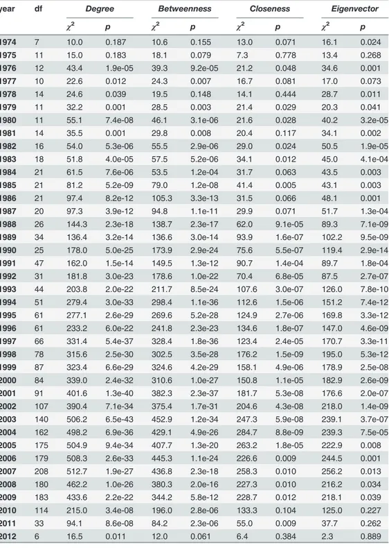
Table 3. Kruskal-Wallis statistics results for the publications case.
year df Degree Betweenness Closeness Eigenvector
χ2 p χ2 p χ2 p χ2 p
1974 7 10.0 0.187 10.6 0.155 13.0 0.071 16.1 0.024
1975 11 15.0 0.183 18.1 0.079 7.3 0.778 13.4 0.268
1976 12 43.4 1.9e-05 39.3 9.2e-05 21.2 0.048 34.6 0.001
1977 10 22.6 0.012 24.3 0.007 16.7 0.081 17.0 0.073
1978 14 24.6 0.039 19.5 0.148 14.1 0.444 28.7 0.011
1979 11 32.2 0.001 28.5 0.003 21.4 0.029 20.3 0.041
1980 11 55.1 7.4e-08 46.1 3.1e-06 21.6 0.028 40.2 3.2e-05
1981 14 35.5 0.001 29.8 0.008 20.4 0.117 34.1 0.002
1982 16 54.0 5.3e-06 55.5 2.9e-06 29.0 0.024 50.5 1.9e-05
1983 18 51.8 4.0e-05 57.5 5.2e-06 34.1 0.012 45.0 4.1e-04
1984 21 61.5 7.6e-06 53.5 1.2e-04 31.7 0.063 43.5 0.003
1985 21 81.2 5.2e-09 79.0 1.2e-08 41.4 0.005 43.1 0.003
1986 21 97.4 8.2e-12 105.3 3.3e-13 31.5 0.066 48.1 0.001
1987 20 97.3 3.9e-12 94.8 1.1e-11 29.9 0.071 51.7 1.3e-04
1988 26 144.3 2.3e-18 138.7 2.3e-17 62.0 9.1e-05 89.3 7.1e-09
1989 34 136.4 3.2e-14 136.6 3.0e-14 93.9 1.6e-07 102.2 9.5e-09
1990 25 178.0 5.0e-25 173.9 2.9e-24 75.6 5.5e-07 119.4 2.9e-14
1991 47 162.0 1.5e-14 149.5 1.3e-12 90.7 1.4e-04 89.7 1.8e-04
1992 31 181.8 3.0e-23 178.6 1.0e-22 70.4 6.8e-05 87.5 2.7e-07
1993 44 203.8 2.0e-22 211.7 8.5e-24 107.6 3.0e-07 126.0 7.8e-10 1994 51 279.4 3.0e-33 298.4 1.1e-36 112.6 1.5e-06 151.2 7.4e-12 1995 61 277.1 2.6e-29 269.6 5.2e-28 124.9 2.7e-06 169.8 3.3e-12 1996 61 233.2 6.0e-22 241.8 2.3e-23 134.6 1.8e-07 147.0 4.6e-09 1997 66 331.4 5.4e-37 328.4 1.8e-36 123.4 2.4e-05 170.7 3.3e-11 1998 78 315.6 2.5e-30 302.5 3.5e-28 176.2 1.5e-09 195.0 5.3e-12 1999 87 323.4 6.6e-29 324.6 4.2e-29 158.1 4.9e-06 178.9 2.5e-08 2000 84 339.0 2.4e-32 310.6 1.0e-27 150.8 1.1e-05 182.9 2.6e-09 2001 91 401.6 1.3e-40 382.3 2.3e-37 181.7 5.3e-08 176.6 2.0e-07 2002 107 390.4 7.1e-34 375.4 1.7e-31 204.6 4.3e-08 218.0 1.4e-09 2003 140 506.2 6.5e-43 452.9 1.2e-34 247.3 5.9e-08 239.1 3.7e-07 2004 162 498.2 6.9e-36 429.1 4.9e-26 284.7 8.8e-09 239.3 7.5e-05 2005 175 504.9 9.4e-34 407.7 1.3e-20 263.2 1.8e-05 222.9 0.008
2006 179 508.3 2.6e-33 445.3 1.1e-24 226.6 0.009 244.5 0.001
2007 208 512.7 1.9e-27 436.8 2.3e-18 258.3 0.010 256.2 0.013
2008 180 462.2 1.0e-26 380.3 2.0e-16 227.3 0.010 216.2 0.034
2009 183 433.6 2.2e-22 344.2 5.8e-12 228.7 0.012 218.1 0.039
2010 114 215.0 3.4e-08 196.0 2.8e-06 133.3 0.104 125.0 0.227
2011 33 94.1 8.6e-08 84.2 2.3e-06 55.0 0.009 37.7 0.262
2012 6 16.5 0.011 12.0 0.061 6.4 0.384 2.3 0.889
samples, in our case, the authors classified into each cluster). Specifically, ANOVA tests the null hypothesis that samples in two or more groups are drawn from populations with the same mean values. In our scenario, this implies testing if the authors classified in the previously cal-culated clusters (responseor dependent variable) are drawn from authors with the same mean values of centrality in the co-authorship network (factoror independent variable). But the
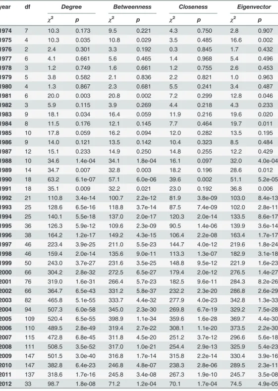
Table 4. Kruskal-Wallis statistics results for the citations case.
year df Degree Betweenness Closeness Eigenvector
χ2 p χ2 p χ2 p χ2 p
1974 7 10.3 0.173 9.5 0.221 4.3 0.750 2.8 0.907
1975 4 10.3 0.035 10.8 0.029 3.5 0.485 16.6 0.002
1976 2 2.4 0.301 3.3 0.192 0.3 0.845 1.7 0.432
1977 6 4.1 0.661 5.6 0.465 1.4 0.968 5.4 0.496
1978 3 1.2 0.749 1.6 0.661 1.2 0.755 2.6 0.453
1979 5 3.8 0.582 2.1 0.836 2.2 0.821 1.0 0.963
1980 4 1.3 0.867 2.3 0.681 5.5 0.241 3.4 0.487
1981 6 20.0 0.003 20.8 0.002 7.2 0.299 12.8 0.046
1982 3 5.9 0.115 3.9 0.269 4.4 0.218 4.3 0.233
1983 9 18.1 0.034 16.4 0.059 11.9 0.216 19.6 0.020
1984 8 11.5 0.176 12.1 0.145 7.7 0.464 19.7 0.011
1985 10 17.8 0.059 16.2 0.094 12.0 0.282 13.5 0.195
1986 9 14.0 0.121 13.5 0.142 10.4 0.323 8.5 0.484
1987 12 15.1 0.233 14.9 0.250 14.8 0.255 12.2 0.429
1988 10 34.6 1.4e-04 34.1 1.8e-04 16.1 0.097 32.0 4.0e-04
1989 14 34.7 0.007 32.8 0.003 18.2 0.196 28.6 0.012
1990 18 63.2 6.1e-07 57.1 6.0e-06 39.6 0.002 51.1 5.2e-05
1991 18 35.1 0.009 32.2 0.021 23.0 0.192 36.8 0.006
1992 21 110.8 3.4e-14 100.7 2.2e-12 81.9 3.8e-09 103.0 8.4e-13
1993 25 128.6 6.5e-16 118.8 3.7e-14 87.5 7.4e-09 102.0 2.8e-11
1994 25 140.1 5.5e-18 137.0 2.0e-17 120.3 2.0e-14 133.5 8.6e-17
1995 36 126.3 5.9e-12 109.6 2.3e-09 90.5 1.4e-06 139.9 3.6e-14
1996 38 164.2 1.2e-17 149.2 4.3e-15 106.4 2.2e-08 163.4 1.7e-17 1997 46 223.4 3.9e-25 211.0 5.5e-23 144.7 4.0e-12 219.6 1.8e-24 1998 46 159.4 2.0e-14 135.6 9.0e-11 113.3 1.3e-07 182.9 3.1e-18 1999 50 243.0 3.7e-27 231.6 3.5e-25 148.8 9.5e-12 221.9 1.6e-23 2000 66 304.2 2.8e-32 272.5 6.5e-27 179.4 2.0e-12 276.5 1.4e-27 2001 76 319.0 1.6e-31 266.4 5.7e-23 182.5 9.6e-11 284.3 8.2e-26 2002 66 364.7 6.5e-43 331.2 5.8e-37 232.2 2.3e-20 286.8 2.6e-29 2003 82 465.8 5.1e-55 333.7 4.4e-32 277.9 4.0e-23 342.8 1.3e-33 2004 94 507.3 6.0e-58 345.0 2.3e-30 269.8 6.7e-19 329.2 7.5e-28 2005 109 520.4 6.5e-55 398.9 1.1e-34 359.6 1.6e-28 369.7 4.4e-30 2006 110 489.5 2.8e-49 319.4 2.7e-22 308.1 1.1e-20 373.5 2.2e-30 2007 115 472.8 6.8e-45 311.8 4.5e-20 251.2 3.7e-12 296.6 5.6e-18 2008 111 508.5 3.5e-52 317.0 1.0e-21 254.4 2.9e-13 325.9 5.4e-23 2009 147 501.5 3.0e-40 316.8 1.7e-14 315.8 2.2e-14 330.4 3.9e-16 2010 147 382.8 6.4e-23 246.8 4.8e-07 238.3 2.8e-06 289.5 2.3e-11 2011 137 318.6 1.7e-16 245.8 3.4e-08 267.3 1.9e-10 245.7 3.5e-08
2012 33 98.7 1.8e-08 71.2 1.2e-04 70.1 1.7e-04 74.5 4.9e-05
reliability of one-way ANOVA results is conditioned, among others assumptions, by normality of the response variables, and the application of the Shapiro-Wilk statistical test [20] revealed that centrality distribution of authors within a cluster is far for being normally distributed. Under these circumstances, we opted for a non-parametric alternative to the one-way ANOVA, the Kruskal-Wallis test [11]. Contrary to one-way ANOVA, which worked with mean values, Kruskal-Wallis tests the null hypothesis that samples in two or more groups are drawn from populations with the same median values. Thus, we applied Kruskal-Wallis test to determine if the centralities of the authors with the same publication (citation) pattern had the same median value and if this value was different from the median value of authors with different publication (citation) patterns. That is, if authors with similar centrality in the network have similar publica-tion (citapublica-tion) patterns and these patterns are different from the ones from authors with different centrality values.
The Kruskal-Wallis statistical results consideringdegree, betweenness, closenessand eigen-vectorcentrality measures for the different years are shown in Tables3and4for publications and citations respectively. Taking the standardα= 0.05 as the significance level for all the Krus-kall-Wallis tests conducted, results revealed that thep-value is lower than the significance value, and therefore the null hypothesis can be rejected for the most relevant cases, those which includes authors whose starting publication date was between 1979 and 2009 (Table 3), for all the centrality with the exception of the closeness centrality during some years between 1979 and 1987. These results are highly conclusive since, for authors who started to publish between 2010 and 2012 (classified into two or more clusters attending to their publications rate), the length of their time series (2 or 3 points) is not enough for obtaining accurate values of similari-ty and, consequently, for a suitable (clustering) classification. A similar situation can be appre-ciated in authors that started to publish before 1978. In this period, there exists a huge
diversity, both in terms of measures and years, in which the null hypothesis cannot be rejected. In any case, and due to the peculiarities of the Google Scholar dataset (that counts publications since 1974) and that Computer Science is a relatively recent discipline, the number of authors that started to publish before 1980 is quite limited with respect to the number of computer sci-entists that started their activity later and these results should not be considered relevant. Again, clustering for this period may not be considered reliable enough. With all of this, the conclusions so far are that (i) in around the 80% of the considered period authors’centrality is highly related with the distribution of publications over time and (ii) the periods in which this relation is not determined correspond to periods in which there are very few authors or periods of temporal series of publications extremely short.
A similar tendency is appreciated in the case of citations (Table 4). Specifically, the null hy-pothesis can be rejected when considering authors that start to receive citations between 1988 and 2012, with exceptions during some years, again when closeness centrality is considered. However, the interval in which we cannot deduce anything about the relation between citation patterns and centrality is extended to authors that started to receive citations between 1974 and 1988. Finally, similar conclusions are drawn when considering different measures of centrality, where there are not differences between authors who started to receive citations in one year or another (except when considering authors that started to receive citations in 1984).
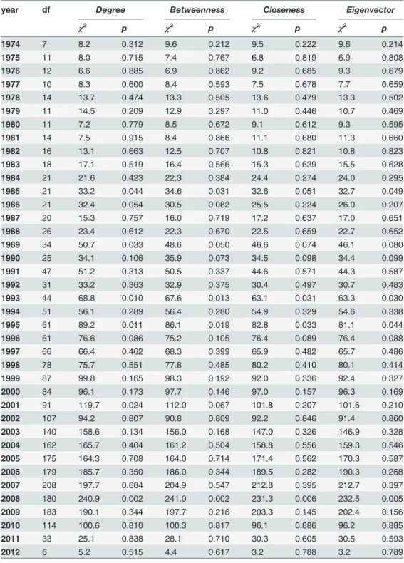
Comparisons with a null model
defined by two parameters: the number of nodes in the graph (n) and the edge probability for drawing an edge between two arbitrary nodes (p). Our random network was obtaining usingn= 57416 (equal to the number of authors simultaneously in both datasets) andp= 1.4e–4 (in order to have a similar level of connection than the original DBLP network), although with different dis-tribution (random). With this test we wanted to exclude the correlation of random collaboration
Table 5. Kruskal-Wallis statistics results for the publications case (using a random graph as a response).
year df Degree Betweenness Closeness Eigenvector
χ2 p χ2 p χ2 p χ2 p
1974 7 8.2 0.312 9.6 0.212 9.5 0.222 9.6 0.214
1975 11 8.0 0.715 7.4 0.767 6.8 0.819 6.9 0.808
1976 12 6.6 0.885 6.9 0.862 9.2 0.685 9.3 0.679
1977 10 8.3 0.600 8.4 0.593 7.5 0.678 7.7 0.659
1978 14 13.7 0.474 13.3 0.505 13.6 0.479 13.3 0.502
1979 11 14.5 0.209 12.9 0.297 11.0 0.446 10.7 0.469
1980 11 7.2 0.779 8.5 0.672 9.1 0.612 9.3 0.595
1981 14 7.5 0.915 8.4 0.866 11.1 0.680 11.3 0.660
1982 16 13.1 0.663 12.5 0.707 10.8 0.821 10.8 0.823
1983 18 17.1 0.519 16.4 0.566 15.3 0.639 15.5 0.628
1984 21 21.6 0.423 22.3 0.384 24.4 0.274 24.0 0.295
1985 21 33.2 0.044 34.6 0.031 32.6 0.051 32.7 0.049
1986 21 32.4 0.054 30.5 0.082 25.5 0.224 26.0 0.207
1987 20 15.3 0.757 16.0 0.719 17.2 0.637 17.0 0.651
1988 26 23.4 0.612 22.3 0.670 22.5 0.659 22.7 0.652
1989 34 50.7 0.033 48.6 0.050 46.6 0.074 46.1 0.080
1990 25 34.1 0.106 35.9 0.073 34.5 0.098 34.4 0.099
1991 47 51.2 0.313 50.5 0.337 44.6 0.571 44.3 0.587
1992 31 33.2 0.363 32.9 0.375 30.4 0.497 30.7 0.483
1993 44 68.8 0.010 67.6 0.013 63.1 0.031 63.3 0.030
1994 51 56.1 0.289 56.4 0.280 54.9 0.329 54.6 0.338
1995 61 89.2 0.011 86.1 0.019 82.8 0.033 81.1 0.044
1996 61 76.6 0.086 75.2 0.105 76.4 0.089 76.4 0.088
1997 66 66.4 0.462 68.3 0.399 65.9 0.482 65.7 0.486
1998 78 75.7 0.551 77.8 0.485 80.2 0.410 80.1 0.414
1999 87 99.8 0.165 98.3 0.192 92.0 0.336 92.4 0.327
2000 84 96.1 0.173 97.7 0.146 97.0 0.157 96.3 0.169
2001 91 119.7 0.024 112.0 0.067 101.8 0.207 101.6 0.210
2002 107 94.2 0.807 90.8 0.869 92.2 0.846 91.4 0.860
2003 140 158.6 0.134 156.0 0.168 147.0 0.326 146.9 0.328
2004 162 165.7 0.404 161.2 0.504 158.8 0.556 159.3 0.546
2005 175 164.3 0.708 164.0 0.714 171.4 0.562 170.3 0.587
2006 179 185.7 0.350 186.0 0.344 189.5 0.282 190.3 0.268
2007 208 197.7 0.684 204.9 0.547 212.8 0.395 212.7 0.397
2008 180 240.9 0.002 241.0 0.002 231.3 0.006 232.5 0.005
2009 183 190.1 0.344 197.7 0.216 203.3 0.145 202.4 0.156
2010 114 100.6 0.810 100.3 0.817 96.1 0.886 96.2 0.885
2011 33 25.1 0.838 28.1 0.710 30.3 0.605 30.5 0.593
2012 6 5.2 0.515 4.4 0.617 3.2 0.788 3.2 0.789
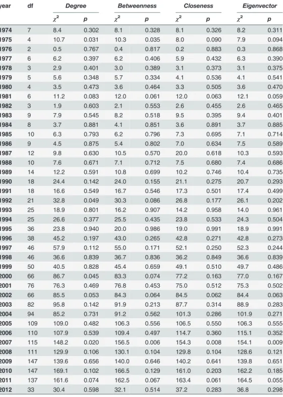
network distributions with our clusters. Results achieved are shown in Tables5and6. According to these tables, both for the publications and citations cases, the null hypothesis cannot be rejected in almost all the the years (in which authors started to publish/receive citations) and for all the dif-ferent centrality measures considered, which confirms the significance of our results.
Table 6. Kruskal-Wallis statistics results for the citations case (using a random graph as a response).
year df Degree Betweenness Closeness Eigenvector
χ2 p χ2 p χ2 p χ2 p
1974 7 8.4 0.302 8.1 0.328 8.1 0.326 8.2 0.311
1975 4 10.7 0.031 10.3 0.035 8.0 0.090 7.9 0.094
1976 2 0.5 0.767 0.4 0.817 0.2 0.883 0.3 0.868
1977 6 6.2 0.397 6.2 0.406 5.9 0.432 6.3 0.390
1978 3 2.9 0.401 3.0 0.389 3.1 0.373 3.1 0.375
1979 5 5.6 0.348 5.7 0.334 4.1 0.536 4.1 0.541
1980 4 3.5 0.473 3.6 0.464 3.3 0.505 3.6 0.470
1981 6 11.2 0.083 12.0 0.061 12.0 0.063 12.1 0.059
1982 3 1.9 0.603 2.1 0.553 2.6 0.455 2.6 0.465
1983 9 7.9 0.545 8.2 0.518 9.5 0.395 9.4 0.401
1984 8 3.7 0.881 4.1 0.851 3.6 0.891 3.7 0.885
1985 10 6.3 0.793 6.2 0.796 7.3 0.695 7.1 0.714
1986 9 4.5 0.875 5.4 0.802 7.0 0.634 7.5 0.589
1987 12 9.8 0.630 10.5 0.570 20.0 0.618 10.3 0.593
1988 10 7.6 0.671 7.1 0.712 7.5 0.680 7.4 0.686
1989 14 12.2 0.591 10.8 0.699 10.2 0.746 10.4 0.735
1990 18 24.4 0.142 24.0 0.155 21.1 0.275 20.7 0.293
1991 18 16.6 0.549 16.7 0.546 17.3 0.501 17.4 0.499
1992 21 32.8 0.049 30.3 0.086 26.8 0.177 26.1 0.202
1993 25 18.9 0.801 16.2 0.907 14.2 0.958 14.0 0.961
1994 25 26.6 0.377 25.5 0.435 23.8 0.533 24.3 0.504
1995 36 23.8 0.940 20.0 0.986 19.0 0.991 18.9 0.991
1996 38 45.2 0.197 43.0 0.265 42.8 0.271 42.8 0.273
1997 46 57.9 0.112 55.0 0.171 52.1 0.250 52.3 0.244
1998 46 36.6 0.839 36.7 0.836 36.2 0.849 36.6 0.839
1999 50 40.5 0.828 45.4 0.659 49.1 0.510 49.7 0.486
2000 66 86.7 0.045 83.3 0.074 77.2 0.163 77.0 0.167
2001 76 76.3 0.469 76.8 0.453 75.0 0.512 75.3 0.502
2002 66 85.5 0.053 84.3 0.064 84.5 0.062 84.4 0.063
2003 82 95.8 0.142 91.9 0.213 87.7 0.314 88.9 0.283
2004 94 85.2 0.731 91.2 0.562 101.3 0.286 101.9 0.271
2005 109 109.0 0.482 106.3 0.556 106.5 0.550 106.3 0.555
2006 110 107.9 0.539 109.4 0.497 114.7 0.360 115.1 0.352
2007 115 148.2 0.020 156.5 0.006 154.3 0.008 154.1 0.009
2008 111 129.9 0.106 130.1 0.104 129.8 0.104 128.6 0.121
2009 147 139.6 0.656 140.0 0.646 140.2 0.641 139.8 0.651
2010 147 169.1 0.102 166.5 0.129 161.0 0.203 162.2 0.185
2011 137 161.6 0.074 162.5 0.067 163.4 0.061 164.5 0.055
2012 33 30.4 0.598 32.1 0.514 37.2 0.283 36.8 0.298
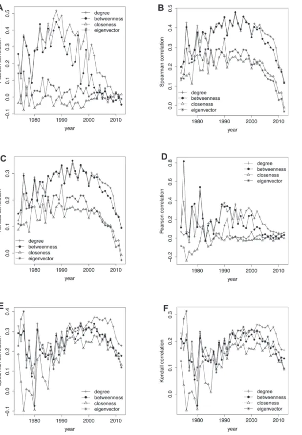
Correlation measures between authors’centrality and their publications (citations) counts. With the aim of testing the relation between authors’centrality in the co-authors net-work and their total number of publications (citations), we calculated three well-known corre-lation indexes: Pearson, Spearman and Kendall.Fig. 2shows the values of the different indexes taking into account different centrality measures (degree, betweenness, closeness and eigenvec-tor centrality) and splitting authors according to the year of their first publication/citation. Re-sults revealed that the correlation between centrality and number of publications (citations) is not significative (lower than 0.5 in almost cases), with the only exception of the authors who started their activity around 1990 when considering the correlation between their publications and degree (betweenness) centrality (Fig. 2AandFig. 2B). This justifies the necessity of consid-ering the whole scholars’timeline as sign of their research activity.
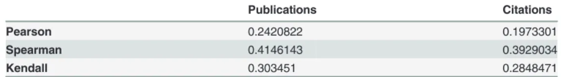
Other experiments without considering time. Finally, we run an experiment to demon-strate the importance of classifying authors according to the year of their first publications/cita-tion when looking for their relapublications/cita-tion with centrality in the co-authorship network. Specifically, we computed the Pearson, Spearman and Kendall correlation indexes between the number of publications/citations and the degree centrality (the one with best results inFig. 2) of all the au-thors in the dataset (independently of the length of their careers). Results inTable 7, with cor-relation values within the ranges of the ones inFig. 2confirm the importance of splitting authors by the year in which their careers started.
Discussion
The main focus of this work is on analysing the importance of collaborations in academic suc-cess over time, by considering sucsuc-cess as the volume of publications and cites to these publica-tions. That is, on analysing if the volume of collaborations of one author together with the relevance of his collaborators is related to his research performance over time. We made use of two different datasets: one obtained by crawling theGoogle Scholarplatform and the other the well-known DBLP dataset. By the application of a two-steps methodology based on (i) cluster-ing scholars’timelines to explore their temporal patterns and (ii) the application of non-parametric statistics to establish the correlation among timeline and centrality, we confirmed our hypothesis that computer scientists’centrality in the co-authorship network is related with the patterns that their publications (citations) followed along the years. Although this relation was found both in the case of publications and citations and independently of the centrality measure, we could not guarantee the existence of relation (i) for scholars that started to lish/receive citations recently (very short time series) neither (ii) for those that started to pub-lish before 1979 in the case of publications (1988 in the case of citations). This relation holds for most of the period considered: this confirms our initial hypothesis that collaboration affects (and is affected by) research performance over time. What is likely is that, the more collabora-tions one author has, the higher his number of publicacollabora-tions will be and the more attention they will receive. Moreover, the relevance of these collaborations seems to play a key role in the in-crease the number of publications and their visibility.
Fig 2. Correlation measures between authors’centrality and their publications (citations) count.(a) Pearson correlation between authors’centrality and their publications count. (b) Spearman correlation between authors’centrality and their publications count (c) Kendall correlation between authors’
centrality and their publications count. (d) Pearson correlation between authors’centrality and their citations count. (e) Spearman correlation between authors’centrality and their citations count. (f) Kendall correlation between authors’centrality and their citations count.
measures, such as cross-clustering coefficient and cross-transitivity [24,25] to conduct social network analysis to see whether more further information could be uncovered. Finally, once temporal series are classified in clusters, it could be interesting to characterise those series ac-cording to the different types of continuous dynamics that they exhibit: periodic, chaotic, and periodic with noisy [26–28].
To conclude, the extension of our study to other disciplines besides Computer Science would give us a better understanding of the dynamics of research. Once discovered these dy-namics, the next logical step should be the development of a prediction framework that allows scholars to improve their collaboration network in order to increase their temporal success.
Supporting Information
S1 Appendix. Anatomy of the Google Scholar dataset. (PDF)
Acknowledgments
This work was partially done while Sandra Servia-Rodríguez was visiting the Computer Labo-ratory of the University of Cambridge.
Author Contributions
Conceived and designed the experiments: SS AN CM AF RPD. Performed the experiments: SS. Analyzed the data: SS. Contributed reagents/materials/analysis tools: SS. Wrote the paper: SS AN CM AF RPD.
References
1. Newman M (2004) Coauthorship networks and patterns of scientific collaboration. Proceedings of the National Academy of Sciences 101: 5200–5205. PMID:14745042
2. Sun X, Kaur J, Milojevi S, Flammini A, Menczer F Social Dynamics of Science. Scientific Reports 3: DOI:10.1038/srep01069.
3. Deville P, Wang D, Sinatra R, Song C, Blondel VD, et al. (2014) Career on the Move: Geography, Strati-fication, and Scientific Impact. Scientific reports 4. doi:10.1038/srep04770PMID:24759743
4. Gargiulo F, Carletti T (2014) Driving forces of researchers mobility. Scientific reports 4. PMID: 24810800
5. Bellotti E (2012) Getting funded. Multi-level network of physicists in Italy. Social Networks 34: 215–
229.
6. Ding Y, Yan E, Frazho A, Caverlee J (2009) Pagerank for ranking authors in co-citation networks. Jour-nal of the American Society for Information Science and Technology 60: 2229–2243.
7. Abbasi A, Altmann J, Hossain L (2011) Identifying the effects of co-authorship networks on the perfor-mance of scholars: A correlation and regression analysis of perforperfor-mance measures and social network analysis measures. Journal of Informetrics 5: 594–607.
8. Abbasi A, Chung KSK, Hossain L (2012) Egocentric analysis of co-authorship network structure, posi-tion and performance. Informaposi-tion Processing & Management 48: 671–679.
Table 7. Correlation measures between authors’centrality and their publications (citations) counts without splitting authors per year of theirfirst publication (citation).
Publications Citations
Pearson 0.2420822 0.1973301
Spearman 0.4146143 0.3929034
Kendall 0.303451 0.2848471
9. Wang J (2013) Citation time window choice for research impact evaluation. Scientometrics 94: 851–
872.
10. Sarigöl E, Pfitzner R, Scholtes I, Garas A, Schweitzer F (2014) Predicting scientific success based on coauthorship networks. arXiv preprint arXiv:14027268.
11. Kruskal WH, Wallis WA (1952) Use of ranks in one-criterion variance analysis. Journal of the American statistical Association 47: 583–621.
12. Jain A, Murty N, Flynn P (1999) Data clustering: a review. ACM Computing Surveys (CSUR) 31: 264–
323.
13. Jain A, Dubes R (1988) Algorithms for clustering data. Prentice-Hall, Inc.
14. Berndt D, Clifford J (1994) Using dynamic time warping to find patterns in time series. In: KDD work-shop. Seattle, WA, volume 10, pp. 359–370.
15. Sakoe H, Chiba S (1978) Dynamic programming algorithm optimization for spoken word recognition. Acoustics, Speech and Signal Processing, IEEE Transactions on 26: 43–49.
16. Sakoe H, Chiba S (1971) A dynamic programming approach to continuous speech recognition. In: Pro-ceedings of the seventh international congress on acoustics. volume 3, pp. 65–69.
17. Langfelder P, Zhang B, Horvath S (2008) Defining clusters from a hierarchical cluster tree: the Dynamic Tree Cut package for R. Bioinformatics 24: 719–720. PMID:18024473
18. Freeman L (1979) Centrality in social networks conceptual clarification. Social Networks 1: 215–239. 19. Miller RG Jr (1997) Beyond ANOVA: basics of applied statistics. CRC Press.
20. Shapiro SS, Wilk MB (1965) An analysis of variance test for normality (complete samples). Biometrika: 591–611.
21. Bollobás B (1998) Random graphs. Springer.
22. Sun X, Kaur J, Possamai L, Menczer F (2011) Detecting ambiguous author names in crowdsourced scholarly data. In: 2011 IEEE Third international conference on Privacy, security, risk and trust (PAS-SAT) and 2011 IEEE Third international conference on Social Computing (socialCom). IEEE, pp. 568–
571.
23. Sun X, Kaur J, Possamai L, Menczer F (2013) Ambiguous author query detection using crowdsourced digital library annotations. Information Processing & Management 49: 454–464.
24. Gao ZK, Zhang XW, Jin ND, Marwan N, Kurths J (2013) Multivariate recurrence network analysis for characterizing horizontal oil-water two-phase flow. Physical Review E 88: 032910. PMID:24125328 25. Gao ZK, Zhang XW, Jin ND, Donner RV, Marwan N, et al. (2013) Recurrence networks from
multivari-ate signals for uncovering dynamic transitions of horizontal oil-wmultivari-ater stratified flows. EPL (Europhysics Letters) 103: 50004. PMID:24125328
26. Xu X, Zhang J, Small M (2008) Superfamily phenomena and motifs of networks induced from time se-ries. Proceedings of the National Academy of Sciences 105: 19601–19605. doi:10.1073/pnas. 0806082105PMID:19064916
27. Zhang J, Small M (2006) Complex network from pseudoperiodic time series: Topology versus dynam-ics. Physical Review Letters 96: 238701. PMID:16803415