www.hydrol-earth-syst-sci.net/12/1189/2008/ © Author(s) 2008. This work is distributed under the Creative Commons Attribution 3.0 License.
Earth System
Sciences
A stochastic approach for the description of the water balance
dynamics in a river basin
S. Manfreda and M. Fiorentino
Dipartimento di Ingegneria e Fisica dell’Ambiente (DIFA), Universit`a degli Studi della Basilicata, via dell’Ateneo Lucano, 10, Potenza, 85100, Italy
Received: 17 January 2008 – Published in Hydrol. Earth Syst. Sci. Discuss.: 13 March 2008 Revised: 9 July 2008 – Accepted: 18 August 2008 – Published: 17 September 2008
Abstract. The present paper introduces an analytical ap-proach for the description of the soil water balance dynam-ics over a schematic river basin. The model is based on a stochastic differential equation where the rainfall forcing is interpreted as an additive noise in the soil water balance. This equation can be solved assuming known the spatial distribu-tion of the soil moisture over the basin transforming the two-dimensional problem in space in a one two-dimensional one. This assumption is particularly true in the case of humid and semi-humid environments, where spatial redistribution becomes dominant producing a well defined soil moisture pattern. The model allowed to derive the probability density function of the saturated portion of a basin and of its relative saturation. This theory is based on the assumption that the soil water storage capacity varies across the basin following a parabolic distribution and the basin has homogeneous soil texture and vegetation cover. The methodology outlined the role played by the soil water storage capacity distribution of the basin on soil water balance. In particular, the resulting probability density functions of the relative basin saturation were found to be strongly controlled by the maximum water storage ca-pacity of the basin, while the probability density functions of the relative saturated portion of the basin are strongly in-fluenced by the spatial heterogeneity of the soil water storage capacity. Moreover, the saturated areas reach their maximum variability when the mean rainfall rate is almost equal to the soil water loss coefficient given by the sum of the maximum rate of evapotranspiration and leakage loss in the soil water balance. The model was tested using the results of a continu-ous numerical simulation performed with a semi-distributed
Correspondence to:S. Manfreda ([email protected])
model in order to validate the proposed theoretical distribu-tions.
1 Introduction
Dynamics of soil moisture in time and space is governed by complex and dynamical interactions between climate, soil and vegetation. Its spatial distribution over a river basin provides a crucial link between hydrological and ecological processes through its controlling influence on runoff gener-ation, groundwater recharge, transpirgener-ation, carbon assimila-tion, etc. The interrelationship between ecological and geo-physical determinants of surface water balance is at the fore-front of a number of outstanding issues in ecohydrological science (e.g. Rodr´ıguez-Iturbe and Porporato, 2004; Mon-taldo et al., 2005).
Recent research has received significant inputs for the de-scription of this variable through the numerous experimental campaigns carried out in the last years (e.g. Monsoon, 1990; Washita, 1992, 1994; SGP, 1997, 1999; Tarrawarra experi-ment). These experiments have increased our understanding of the temporal variability and of the spatial structure of the soil moisture fields and of the importance of physical charac-teristics such as soil texture, vegetation and topographic pat-terns for soil moisture variability (Western et al., 2002; Kim and Barros, 2002; Wilson et al., 2004; Jawson and Niemann, 2007).
These theories have been useful to describe the vegeta-tion water stress in a probabilistic framework (Porporato et al., 2001) and to investigate on the interactive manner by which resource availability are manifested within various ecological systems observed in nature (e.g. van Wijk and Rodr´ıguez-Iturbe, 2002; Scanlon et al., 2005; Caylor et al., 2005).
Recent studies have extended the theoretical description of the soil moisture to the spatial scale introducing a space-time soil moisture model driven by a stochastic space-space-time rainfall forcing described by a sequence of circular cell of Poisson rate (Isham et al., 2005; Rodr´ıguez-Iturbe et al., 2006; Manfreda et al., 2006). The methodology explicitly ac-counts for soil characteristics, vegetation patterns, and rain-fall dynamics neglecting topographical effects and the upper bound due to soil saturation. This soil moisture model can be considered representative of a relatively flat landscape under arid/semiarid climatic conditions.
The description of the soil moisture evolution over a river basin is, at the moment, a challenging topic that may be useful for both ecohydrological and hydrological research. Some examples in this direction are given in the paper by Botter et al. (2007a), where the probability density func-tions of the slow components of the runoff are derived us-ing a river basin schematization with uniform macroscopic parameters governing the soil water balance neglecting the spatial heterogeneity of soil properties. The same authors ex-tended the previous work introducing the spatial heterogene-ity of the basin summing the runoff contributions provided by different subbasins with spatially averaged soil properties (Botter et al., 2007b), but still each subbasin is considered as an homogeneous entity where the relative saturation follows the same dynamics of a point process.
The present work represents an attempt to fill such a gap introducing a mathematical schematization for the derivation of the probability distribution of the relative saturation of a basin accounting for the spatial heterogeneity in soil water storage capacity. The proposed scheme includes a number of approximations, but it leads to an interesting framework for the derivation of the main statistics of basin scale variables. Among others, our interest focused on the behaviour of rela-tive saturation and saturated areas over a river basin that may be responsible of the dynamics of riparian vegetation as well as runoff generation.
The theory is based on the conceptual Xinanjiang model that describes watershed heterogeneity using a parabolic curve for the distribution of the soil water storage ca-pacity (Zhao et al., 1980). The Xinanjiang model was first developed in 1973 and published in English in 1980. It is a well-known lumped watershed model widely used in China. Furthermore, the adopted relationship between the extent of saturated areas and the volume stored in the catchment has driven the evolution of a number of more recent models such as the Probability Distributed Model (Moore and Clarke, 1981; Moore, 1985, 1999), the
VIC model (Wood et al., 1992) and the ARNO model (To-dini, 1996).
The present paper provides a description of the mathemat-ical framework used to derive the probability density func-tions of the soil water content and of the portion of saturated areas at basin scale in Sects. 2 and 3. Results of the the-ory along with an application of the model are discussed in Sect. 4 that precedes the conclusions.
2 Model description
2.1 Rainfall model
Rainfall occurrences are modelled by a sequence of instanta-neous pulses that occur in a Poisson process of rateλin time and uniform in space. Each pulse is characterized by a ran-dom total depthhexponentially distributed with meanαthat may be considered as the mean daily rainfall since the model is interpreted at the daily time scale (see Rodr´ıguez-Iturbe et al., 1999).
In the following, we will refer to a normalized version of the density function of rainfall depths described as
fH(h)=γ e−γ h (1)
whereγ=wmax/αandwmaxis the maximum value of the soil water storage capacity in the basin.
The spatial heterogeneity of rainfall is neglected assuming uniform distribution of rainfall occurring at random in time over the entire basin. Such an assumption may be more or less reliable depending on climatic characteristics of rainfall forcing and basin size. In general, one should expect that it becomes more realistic for medium/small size basins. The climatic conditions may also affect the spatial correlation and the extend of rainfall fields that become more and more uni-form in humid regions.
2.2 The variability of the soil water storage capacity over the basin
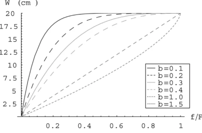
The watershed heterogeneity is described using a parabolic curve for the water storage capacity of the soil (Zhao et al., 1980)
f F=1−
1− W
wmax b
(2) wheref/F represents the fraction of the basin with water storage capacity≤W,wmaxis the maximum value of the wa-ter storage capacity in the basin andb is a shape parameter that according to Zhao (1992) assumes values between 0.1– 0.4 increasing with the characteristic dimension of the basin. An example of the Eq. (2) is given in Fig. 1 where this func-tion is plotted for different values ofb. The parameterb af-fects the spatial heterogeneity ofWthat increases with larger values ofband becomes a uniform distribution whenb=0.
The above distribution has been extensively used in several conceptual models where the parametersb and wmaxhave been calibrated against runoff data.
A first attempt to seek for a physical interpretation of the parameters b and wmax was made by Sivapalan and Woods (1995). In this work, the authors observed a qual-itative connection between the landform types and the soil depths of a basin in Western Australia to the topographic po-sition. Later on, Sivapalan et al. (1997) developed a concep-tual rainfall/runoff model along the lines of the VIC model (Wood et al., 1992) exploiting the topographic index of the TOPMODEL (WI=ln(a/t anβ) by Beven and Kirkby, 1979)
to define the parameters of Eq. (2).
In a more recent work, Chen et al. (2007) stated that Eq. (2) can be estimated directly from digital el-evation data. In particular, they use the spatial dis-tribution of the TOPMODEL topographic index to esti-mate the so called index of runoff generation difficulty (IRDG=(max[WI]−WI)/(max[WI]−min[WI])) through a
normalized function of the topographic index as suggested by Gou et al. (2000). Specifically, the authors propose to substitute the parabolic curve of soil water storage capacity of the Xinanjiang model with the cumulative frequency dis-tribution of IRDG. Under this hypothesis one can estimate the shape parameterbby fitting Eq. (2) with the cumulative frequency distribution of IRDG.
In the following, we provide a sequence of definitions use-ful for model description and comprehension.
The total water storage capacity of the basin is obtained integrating (1−f/F) betweenW=0 andwmax, obtaining WM=wmax
1+b, (3)
that according to Zhao (1984) and Zhao and Wang (1988) assumes values between 120 mm and 160 mm depending on the climatic zone.
In order to obtain a water balance equation with only one state variable, it is necessary to make the hypothesis that the soil water distribution is known over the basin. In partic-ular, it is possible to assume that the soil water content is
0.2 0.4 0.6 0.8 1 fF 2.5
5 7.5 10 12.5 15 17.5 20 W cm
b1.5 b1.0 b0.4 b0.3 b0.2 b0.1
Fig. 1. Distribution of the water storage capacity of a river basin assumingwmax=20 cm, while the parameterbchanges from 0.1 to 1.5.
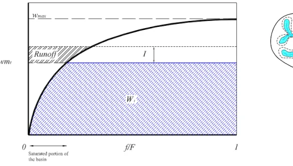
redistributed within the basin cumulating in the areas with lower soil depth following the same assumption of the Xi-nanjiang model. The conceptual schematization of the basin is sketched in Fig. 2, where both the soil water content dis-tribution and the soil water storage capacity are described. From this graph, it is also clear that the relative saturated ar-eas,a, are described by the same relationship given in Eq. (2) whereacorrespond to the ratiof/F.
The watershed-average soil moisture storage at timet, is the integral of 1−f/F between zero and the actual value of the water level in the basin scheme,wmt,
Wt= Z wmt
0
1−f F
dW=W M 1−
1−wmt
wmax 1+b!
. (4)
The relative saturation of the basin is a significant vari-able to interpret the basin dynamics and it will be considered, from now on, the state variable of the system along with the saturated portion of the basin,a. The relative saturation of the basin may be defined as the ratio between the total wa-ter content of the basin divided by the total wawa-ter storage capacity. Under the described schematization, the relative saturation of the basin,s, can be defined as
s=Wt W M=
1−1−wmt wmax
1+b
. (5)
2.3 The soil water losses
Fig. 2.Schematization of the basin structure and soil water content distribution. The black line represents the distribution of the soil water storage capacity,W, that ranges from 0 towmax; the blue line depicts the water distribution over the schematic basin whose level iswmt;
the dashed line depicts the increase inwmt after a rainfall event producing an infiltrationIover the unsaturated portion of the basin, while
the saturated and the becoming saturated portion of the basin will produce a runoff represented by the dashed area of the graph.
function where the soil losses are assumed to be proportional to the relative saturation of soil in a point
L(ζ )=V ζ (t, x), (6)
whereL(ζ )is the soil water loss relative to the relative soil saturationζ (t, x)at timet in the pointx in space, andV is the water loss coefficient.
It is worth nothing to remark that the same loss func-tion has been used by numerous authors (e.g. Entekhabi and Rodr´ıguez-Iturbe, 1994; Pan et al., 2003; Porporato et al., 2004; Rodr´ıguez-Iturbe et al., 2006) essentially for two rea-sons: first of all, it represents a reasonable approximation for the sum of the actual evapotranspiration and the leakage and second it is a useful simplification in a mathematical frame-work.
Since the adopted soil loss function is linear, it may be generalized at the basin scale using the product between the relative basin saturation,s, and the water loss coefficient. It follows
Lb(wmt)=V s=V 1−
1−wmt wmax
1+b!
. (7)
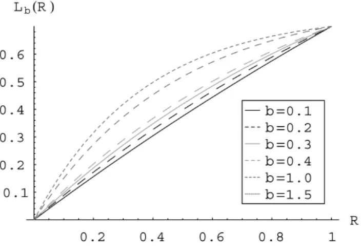
For analytical purposes, the soil water losses can be ex-pressed as a function of the relative water level in the basin expressed through the ratioR=wmt
wmax. In this case, the soil water losses are computed, using an approximated exponen-tial function, as
Lb
R=wmt wmax
∼ =V
e−kR−1
e−k−1
(8)
wherekis a coefficient that has been used to fit the above with Eq. (7). The two functions were fitted imposing the condition that they subtend the same area betweenR=0 and 1. Using this assumption, one may obtain the following ex-pression
b=2−2e
k+k+ekk
ek−k−1 , (9)
that may be solved numerically ink providing an estimate of k as a function of the parameter b. This yields k ∼= b/b7−1
3
.
The Eq. (9) is represented in Fig. 3 for different values of the parameterbthat varies from 0.1 up to an hypotheti-cal value of 1.5. This graph shows how the soil water loss function at the basin scale becomes more non-linear with the increase of the values ofb.
3 The water balance equation
The water balance equation needs to be written at the basin scale in order to derive the relative dynamics of soil water. This problem can tackled working with the mass conserva-tion equaconserva-tion of total water,Wt, or with the water level in the
Using the above approximations for the rainfall forcing and for the spatial distribution of the soil water storage ca-pacity, the soil water balance over the basin can be described through the following stochastic differential equation inwmt
dwmt
dt =I−V s, (10)
whereI represents an additive term of infiltration and water losses are assumed to be proportional to the relative satura-tion of the basins. The advantage to solve the water balance equation inwmtis that the infiltration rate can be summed as
an additive term of the stochastic differential equation. The water levelwmtin the basin schematization increases as long
as the infiltration does not exceed the maximum water stor-age capacity of the basinwmax, but this does not mean that there no runoff production. The infiltration is equal to the rainfall depth in the portion of the basin that have a resid-ual water storage capacity available to be filled, there after the rainfall will be converted into runoff (see Fig. 2). The schematization, in fact, accounts for the upper bound im-posed by the soil saturation.
In the present scheme, the runoff generation occur for sat-uration excess in the saturated portion of the basin obtain-ing a behaviour comparable with a Dunne mechanism where the direct precipitation on saturated areas (saturated overland flow) is dominant runoff generation mechanisms (e.g. Hib-bert, 1967; Dunne and Black, 1970).
The water balance equation can be solved using the stan-dardized variable
R=wmt wmax
, (11)
whereR∈[0,1]that represents the relative water level in the parabolic reservoir describing the basin.
Under these assumptions, it is convenient to standardize the soil water loss rate
ρ(R)=β
e−kR−1
e−k−1
, (12)
whereβ=V /(wmax)is the normalized soil water loss coeffi-cient.
The water balance equation becomes
dR
dt =
I wmax
−ρ(R). (13)
Following Rodr´ıguez-Iturbe et al. (1999), the probability density function (PDF) ofRcan be obtained and solved ana-lytically for steady-state conditions. The PDF ofR, obtained using the simplified loss functionρ(R)in the water balance equation above, becomes
p(R)=ρ(R)C e−γ R+λ
R 1
ρ(R)du=
Cek(R−1)−Rγ ek−1
ekR−1
λ(1−e−k ) kβ −1
β ,
(14)
0.2 0.4 0.6 0.8 1
R 0.1
0.2 0.3 0.4 0.5 0.6
LbR
b1.5 b1.0 b0.4 b0.3 b0.2 b0.1
Fig. 3. Soil water losses computed at the basin scale as a function of the ratioR=wmt
wmax.
whereC is a constant of integration that may be computed simply imposing the normalizing condition,R1
0 p(R)dR=1.
Thus,Cassumes the following value
C=1/R1 0
ek(−1+R)−Rγ ek−1
ekR−1−1+λ−e
−k λ kβ
β dR
(15)
C= β
Ŵ[1−γ k]Ŵ
λ−e−k λ kβ
kek Ŵ
kβ−βγ+λ−e−k λ kβ
+
F1
"
1−γ k,1+
(e−k−1)λ kβ ,2−
γ k,ek
#
eγ (γ−k)
·
1
(−1) λ−e−k λ
kβ (ek−1)
(16)
whereŴ[.]is the complete Gamma Function andF1[., ., ., .] is the Hypergeometric Function (Abramowitz and Stegun, 1964; Prudnikov et al., 1986).
According to Eq. (2), the water level in the parabolic reser-voir proposed to describe the soil water storage capacity can be related to the fraction of saturated areas,a, as
wmt=(1−(1−a)
1
b)wmax, (17)
0
100
200
300
400
500
600
700
800
900
0
0.1
0.2
0.3
0.4
0.5
0.6
0.7
Time [days]
P
o
rt
io
n
o
f
S
at
u
rat
ed
A
re
a
s
o
f
th
e
B
a
si
n
w
max=40cm,
b
=0.1
w
max=10cm,
b
=0.1
w
max=40cm,
b
=0.4
w
max=10cm,
b
=0.4
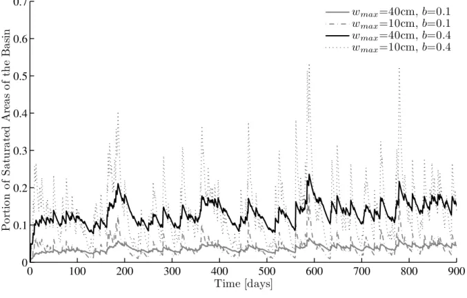
Fig. 4.Temporal dynamics of saturated areas for different values ofwmaxandbreproduced by a numerical simulation performed at the daily time-scale. The remaining parameters areλ=0.3,α=1.0 cm andV=0.7 cm/day.
3.1 Probability density function of saturated areas of the basin
Under these hypotheses, it is possible to define the probabil-ity distribution of saturated areas given the climatic forcing and the geomorphologic characteristics of the basin. In par-ticular, the probability density function ofacan be obtained from the probability density function ofRas
pA(a)=pR(f−1(a))
df−1(a)
da . (18)
To this end, it is necessary to clarify the relationship be-tweenRanda that may be obtained from Eq. (2) where the ratiof/Fmay be also interpreted as the saturated portion of the basin. It follows
R=f−1(a)=1−(1−a)1b. (19)
The derivative off−1(a)is
df−1(a)
da =
1
b(1−a)
1
b−1. (20)
Consequently, using the Eq. (19) one obtains the following expression for the probability density function of the relative saturated areas of a basin
pA(a)=(1−a)
1
b−1
bβ Ce
γ
(1−a)1b−1
−(1−a)1bk ·
ek−1
ek−(1−a)1bk−1 λ−e
−k λ kβ −1
.
(21)
3.2 Probability density function of the relative saturation of the basin
The relative saturation of the basin can be easily charac-terized at this point using the probability distribution of Eq. (14). Then, one can use the relationship betweenR and
s,
R=g−1(s)=(1−(1−s)1+1b), (22)
be used where one also need the derivative of the function
g−1(s)
dg−1(s)
ds =
(1−s)1+1b−1
1+b . (23)
The probability density function for the relative saturation of the basin at the steady state can be described by the fol-lowing expression
p(s)=(1−s) −b
1+bC (1+b)β e
k−1
ek−k(1−s)
1 1+b
−1 λ−e
−k λ kβ −1
·
e
−k(1−s)1+1b+γ
(1−s)1+1b−1
.
(24)
4 Results and discussion
The model proposed here is a minimalist representation of soil moisture dynamics at basin scale. In the following appli-cations the derived PDFs are tested using Monte Carlo sim-ulations in order to understand the reliability of the adopted simplification for the analytical derivation and also to evalu-ate the ability of the model to reproduce the dynamics of a river basin. Results show that the model provides a realistic description of the basin water balance under a wide range of climatic and physical conditions.
In order to show the dynamics of the relative saturated portion of the basin, a numerical simulation of the described model with no approximation in the soil water loss function was performed over a temporal window of 100 years using different values ofbandwmax. A realization of the process is given in Fig. 4 considering a limited temporal window of 900 days. Different parameters of the soil water storage capacity distribution may change dramatically the dynamics of the system and this is even more clear in the PDFs ofa
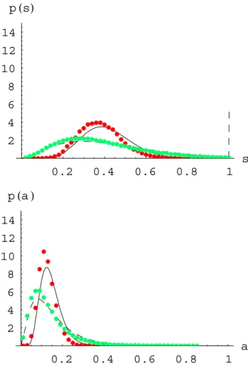
andsdescribed in the following paragraphs. The simulation has been used for comparison with the theoretical distribu-tions obtaining a very good agreement as one may observe in Fig. 5. The two probability density functions of the rela-tive saturation and the relarela-tive portion of the saturated areas of the basin are compared with the PDFs obtained via nu-merical simulation. This result provides an idea of the errors associated with the use of an approximated function to de-scribe the soil water losses (see Eq. 9).
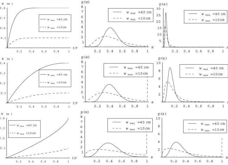
Figure 6 describes a sequence of probability distributions of the relative saturation of the basin and of the saturated ar-eas assuming different set of parameters for the distribution of water storage capacity with fixed climatic conditions. It may be immediately appreciated how the relative structure of the basin plays a fundamental role in the dynamics ofs
anda. It is interesting to note that on one hand the reduc-tion of the maximum water storage capacity,wmax, increases the variability of both relative basin saturation and saturated
0.2
0.4
0.6
0.8
1
s
2
4
6
8
10
12
14
p
s
0.2
0.4
0.6
0.8
1
a
2
4
6
8
10
12
14
p
a
Fig. 5. Comparison between the probability density functions of the relative saturation of the basin (upper graph) and relative satu-rated areas (bottom) obtained with the theoretical distribution given in Eqs. (21) and (24) and numerical simulation (full circles). The parameters adopted arewmax=40 cm (continuous line) and 10 cm (dashed line), while the remaining areb=0.4,λ=0.3,α=1.0 cm and V=0.7 cm/day.
areas; on the other hand the increase of the heterogeneity in the distribution ofW, dictated by the parameterb, does not provide significant change ons. In fact, the increase of the exponentbdoes not apparently affect the variance ofs, but at the same time it increases the mean and the variability of the saturated areas.
0.2 0.4 0.6 0.8 1 fF 0.1
0.2 0.3 0.4
W m
wmax 10 cm wmax 40 cm
0.2 0.4 0.6 0.8 1 s 1
2 3 4 5 6 7 8 ps
wmax 10 cm wmax 40 cm
0.2 0.4 0.6 0.8 1
a 5
10 15 20 25 30
pa
w max 10 cm w max 40 cm
0.2 0.4 0.6 0.8 1
fF 0.1
0.2 0.3 0.4
W m
wmax 10 cm wmax 40 cm
0.2 0.4 0.6 0.8 1 s 1
2 3 4 5 6 7 8 ps
wmax 10 cm wmax 40 cm
0.2 0.4 0.6 0.8 1
a 2
4 6 8 10
pa
w max 10 cm
w max 40 cm
0.2 0.4 0.6 0.8 1
fF 0.1
0.2 0.3 0.4
W m
wmax 10 cm wmax 40 cm
0.2 0.4 0.6 0.8 1 s 1
2 3 4 5 6 7 8 ps
wmax 10 cm
wmax 40 cm
0.2 0.4 0.6 0.8 1
a 2
4 6 8 10
pa
w max 10 cm
w max 40 cm
Fig. 6. Probability density functions of the relative saturation (second column) and of the saturated areas (third column) of a river basin assumingwmaxequal to 40 cm and 10 cm, while the parameterbvaries between 0.1, 0.4 and 1.5 in the top down order. The remaining parameters areλ=0.3,α=1.0 cm andV=0.7 cm/day. In the first column, the soil water storage capacity distribution is represented for the corresponding set of parameterswmaxandbon each row.
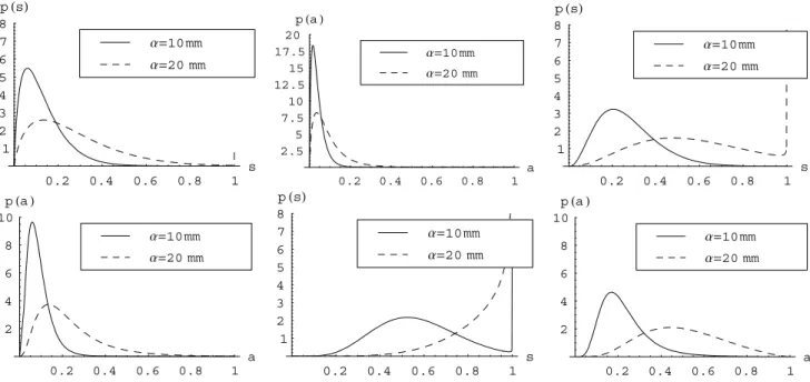
marked change in the PDF’s shape even under the same mean rainfall rate. In fact, one may compare the dashed PDF in the first panel on the left, obtained assuming the parame-tersα=20 mm andλ=0.1 event/day producing a mean rain-fall rate of 2 mm/day, with the PDF in the second panel on the left (continuous line) obtained with parametersα=10 mm andλ=0.2 event/day characterized by the same rainfall rate. The two distribution are slightly different and in particular it seems that the increase in the mean rainfall depth of the storms increases the variability of the relative saturation of the basin. This effect is even more marked in the PDFs of relative saturated areas.
The mean and the standard deviation of the saturated areas,
a, are described in Fig. 8 as a function of the water loss co-efficientV. Generally, the mean value of the basin saturated areas decrease with the increase of the water loss coefficient. A different behaviour is observed for the standard deviation
that reaches a maximum value when the soil water losses coefficient is equal to the mean daily rainfall (here equal to
αλ=3 mm). One may also observe that the presence of a more heterogeneous soil water storage capacity (b=0.4) induces a higher mean but also a higher variability.
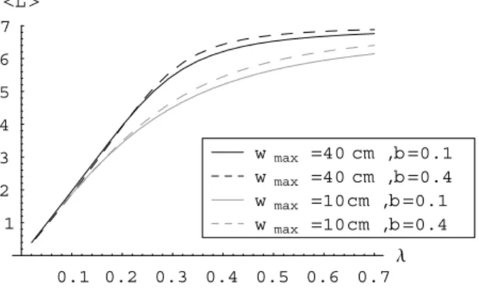
The parameterswmaxandb may also affect the partition between runoff and soil water losses that is described in Fig. 9 as a function of the Poisson rate of rainfallλ. The gen-eral signal is an increase of the soil losses with the increase of the incoming rainfall. Of course some differences may be observed for the different basin configuration considered herein. It may be noticed that the increase of the parameter
0.2 0.4 0.6 0.8 1 s 1
2 3 4 5 6 7 8
ps
Α20 mm Α10 mm
0.2 0.4 0.6 0.8 1 a 2.5
5 7.5 10 12.5 15 17.5 20
pa
Α20 mm Α10 mm
0.2 0.4 0.6 0.8 1 s 1
2 3 4 5 6 7 8 ps
Α20 mm Α10 mm
0.2 0.4 0.6 0.8 1 a 2
4 6 8 10
pa
Α20 mm Α10 mm
0.2 0.4 0.6 0.8 1 s 1
2 3 4 5 6 7 8
ps
Α20 mm Α10 mm
0.2 0.4 0.6 0.8 1 a 2
4 6 8 10
pa
Α20 mm Α10 mm
Fig. 7. Probability density functions of the relative saturation (first column) and of the saturated areas (second column) of a river basin assumingwmaxequal to 20 cm, the parameterb=0.4 and two different values forα(10 mm and 20 mm), while the parameterλ varies between 0.1, 0.2 and 0.4 in the top-down order.
2 4 6 8 10
V 0.2
0.4 0.6 0.8 1
a
w max 10cm ,b0.4
w max 10cm ,b0.1
w max 40 cm ,b0.4
w max 40 cm ,b0.1
2 4 6 8 10
V 0.1
0.2 0.3 0.4
Σa
w max 10cm ,b0.4
w max 10cm ,b0.1
w max 40 cm ,b0.4 w max 40 cm ,b0.1
Fig. 8. Expected value and standard deviation of the saturated areas of the basin as a function of the soil water loss coefficient,V , for different values ofwmaxandb. Remaining parameters are the same of Fig. 6.
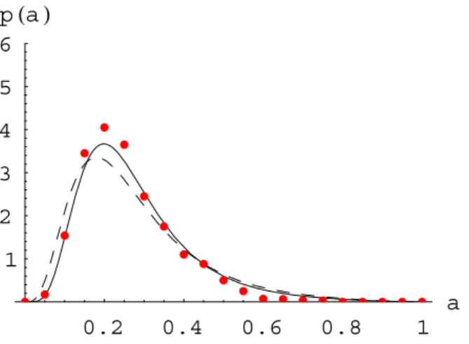
4.1 Comparison of the theoretical model with a continuous numerical simulations
The model has been tested using the data obtained from a continuous hydrological simulation performed using a semi-distributed hydrological model (DREAM – Man-freda et al., 2005) in cascade with a rainfall generator (IRP – Veneziano et al., 2002). Montecarlo simulations were performed over 800 years using synthetic rainfall spatially
proposed theoretically derived PDFs.
Among the two basins investigated by Fiorentino et al. (2007), the Agri represents a perfect study case belong-ing to a humid area suitable to be interpreted through the proposed mathematical model. This basin has been deeply investigated in previous studies and its detailed description is available in Fiorentino et al. (2006, 2007). Consequently, the modelling results obtained for this basin are used here to test the reliability and applicability of the probability distribution of saturated areas derived in the present paper.
Parameters of the theoretical distribution have been com-puted exploiting as much as possible the available informa-tion on the Agri River basin. In particular, rainfall parameters have been estimated from rainfall records during the wet sea-son, the parameterV is estimated from the equation proposed by Pan et al. (2003),
V=max(1,6.08+0.40Ks−0.51LAI )[mm/day], (25)
whereKs=6.06 cm/h (mean value of the permeability over
the basin) and LAI=1.28 (mean value over the basin during the wet season). The parameterbwas fitted using the method proposed by Chen et al. (2007) exploiting the topographic index computed from a digital elevation model at 240 m of resolution obtaining an estimate ofb=0.39.
The comparison between the PDFs of saturated areas ob-tained with the two procedures is depicted in Fig. 10 where the theoretical distributions have been plotted using two dif-ferent values for the parameterwmax derived from Eq. (3) using the two extremes that the total water storage capacity,
W M, can assume according to Zhao (1984) and Zhao and Wang (1988). Both the theoretical PDFs have a good agree-ment with the results obtained from the simulation performed with the DREAM model. Of course, the semi-empirical pa-rameterwmaxshould be estimated from runoff data in order to get a more accurate estimate ofp(a), but this preliminary results shows a low variability of this distribution respect to the range of variability assumed by this last parameter.
5 Conclusions
In the present paper, a new approach is introduced to de-scribe analytically the relative soil saturation of a river basin and the dynamics of its saturated areas. The method pro-vides a simplified description of river basin characteristics, but includes the effect of spatial variability of water storage capacity adopting the same schematization used by Zhao et al. (1980) for the Xinanjiang model.
In summary, this approach allowed to:
– Derive analytically the probability density function of the saturated portion of a basin also called runoff source areas that represent a significant variable in the dynam-ics of a river basin (e.g. Fiorentino et al., 2007). Fur-thermore, the model introduced may be easily adopted
0.1 0.2 0.3 0.4 0.5 0.6 0.7
Λ 1
2 3 4 5 6 7
L
w max 10cm ,b0.4 w max 10cm ,b0.1 w max 40 cm ,b0.4 w max 40 cm ,b0.1
Fig. 9. Expected value of the soil water losses<L>as a function of the parameterλassuming different values forwmaxandb. The remaining parameters areλ=0.3,α=2.0 cm andV=0.7 cm/day.
to derive the probability density function of runoff production as it will be described in a subsequent pa-per by Manfreda (2008)1.
– Derive the probability density function of the relative saturation of a river basin characterized by a given cli-matic forcing and distribution of the soil water storage capacity.
– Identify the role of climatic and physical features of the basin on its soil water dynamics in humid environments through the use of physically meaningful parameters (α,
λandV) and semi-empirical parameters (bandwmax). In this context, an interesting results was observed in the variability of saturated areas that apparently reached its maximum when the soil water loss coefficient gets close to the mean rainfall rate.
– Understand the role played by the distribution of the soil water storage capacity on soil water of the basin. In particular, results outlined a strong control of the spatial heterogeneity on the shape of the probability distribu-tion of saturated areas, while the relative saturadistribu-tion of the basin seems more controlled by the maximum water storage capacity.
– Define a theoretical framework useful also for the de-velopers and numerous users of the Xinanjiang model and similar conceptual models.
The model has been tested with the results of a continu-ous numerical simulation performed with a distributed model obtaining a good agreement between the two outcomes. The exercise reported here was particularly useful to design a strategy for the parameter estimation of the model that turn out to be straightforward.
1Manfreda, S.: Runoff Production Dynamics within a Humid
0.2
0.4
0.6
0.8
1
a
1
2
3
4
5
6
p
a
Fig. 10.Comparison between the probability distribution of the sat-urated areas of the Agri River basin obtained from numerical simu-lation with a semi-distributed model (full circles) and the theoretical density functions derived in the present work where the parameters are:λ=0.29,α=1.35 cm,V=0.606 cm/day,b=0.39 and finallywmax is assumed equal to 16.6 cm (dashed line) and 22.2 cm (continuous line).
The model has not been applied to a real case yet, but a specific experiment has been designed in order to derive the statistics of the averaged soil moisture over a basin hill-slope in order to compare the derived PDFs to a real case. Moreover, the proposed scheme can be used to derive the probability density function of the runoff production at basin scale taking into to account two relevant phenomena like the non-linearity in the rainfall-runoff generation mechanisms and the saturation effect of the basin (Manfreda, 20081).
Appendix A Notation
afraction of saturated areas [dimensionless].
Cconstant of integration [dimensionless].
F1[., ., ., .]hypergeometric function.
f/Fsaturated portion of the basin [dimensionless].
Ŵ[.]complete gamma function.
Iinfiltration [cm].
Lb(R)soil water loss function at the basin scale [cm d−1].
R=wmt
wmax relative water level in the basin [dimensionless].
srelative saturation of the basin [dimensionless].
kcoefficient of the simplified soil water loss function used to fit Eq. (7) [dimensionless].
Wwater storage capacity at a point [cm].
WIwetness index [ln(m)].
wmax maximum value of the water storage capacity in the basin [cm].
wmtwater level in the parabolic reservoir [cm].
Wttotal water content [cm].
V water loss coefficient [cm d−1].
β=V /(wmax) is the normalized soil water loss coefficient [dimensionless].
γ=wmax/α is the normalized mean rainfall depth [dimensionless].
αmean depth of rainfall events [cm].
λrainfall rate per unit time [d−1].
ρ(R)simplified water loss function.
Acknowledgements. This study was supported by the MIUR (Italian Ministry of Instruction, University and Research) under the grant PRIN CoFin2005 entitled “Climate-soil-vegetation interaction in hydrological extremes”. S. Manfreda gratefully acknowledges the support of the CARICAL foundation for his research activities.
Edited by: M. Sivapalan
References
Abramowitz, M. and Stegun, I. A.: Handbook of Mathematical Functions with Formulas, Graphs, and Mathematical Tables, New York, Dover, 1046 pp., 1964.
Arnold, L.: Stochastic Differential Equations: Theory and Applica-tions, John Wiley & Sons, New York, 228 pp., 1974.
Beven, K. J. and Kirkby, M. J.: A physically-based variable con-tributing area model of basin hydrology, Hydrol. Sci. B., 24(1), 43–69, 1979.
Botter, G., Porporato, A., Rodr´ıguez-Iturbe, I., and Rinaldo, A.: Basin-scale soil moisture dynamics and the probabilistic char-acterization of carrier hydrologic flows: leaching-prone com-ponents of the hydrologic responce, Water Resour. Res., 43, W02417, doi:10.1029/2006WR005043, 2007a.
Botter, G., Porporato, A., Daly, E., Rodr´ıguez-Iturbe, I., and Ri-naldo, A.: Probabilistic characterization of base flows in river basins: Roles of soil, vegetation, and geomorphology, Water Re-sour. Res., 43, W06404, doi:10.1029/2006WR005397, 2007b. Caylor, K. K., Manfreda, S., and Rodr´ıguez-Iturbe, I.: On the
cou-pled geomorphological and ecohydrological organization of river basins, Adv. Water Resour., 28(1), 69–86, 2005.
Chen, X., Chen, Y. D., and Xu, C.-Y.: A distributed monthly hydro-logical model for integrating spatial variations of basin topogra-phy and rainfall, Hydrol. Process., 21(2), 242–252, 2007. Dunne, T. and Black, R.: An Experimental Investigation of Runoff
Production in Permeable Soils, Water Resour. Res., 6(2), 478– 490, 1970.
Entekhabi, D. and Rodr´ıguez-Iturbe, I.: An analytic framework for the characterization of the space-time variability of soil moisture, Adv. Water Resour., 17, 25–45, 1994.
Fiorentino, M., Gioia, A., Iacobellis, V., and Manfreda, S.: Analysis on flood generation processes by means of a continuous simula-tion model, Adv. Geosci., 7, 231–236, 2006,
http://www.adv-geosci.net/7/231/2006/.
Guo, F., Liu, X. R., and Ren, L. L.: Topography based water-shed hydrological model-TOPOMODEL and its application, Ad-vances in Water Science, 11(3), 296–301, 2000 (in Chinese). Hewlett, J. D. and Hibbert, A. R., Factors affecting the response
of small watersheds to precipitation in humid areas, in: Forest Hydrology, edited by: Sopper, W. E. and Lull, H. W., Pergamon Press, 275–290, 1967.
Isham, V., Cox, D. R., Rodr´ıguez-Iturbe, I., Porporato, A., and Man-freda, S.: Mathematical characterization of the space-time vari-ability of soil moisture, Proc. R. Soc. Lon. Ser.-A., 461(2064), 4035–4055, 2005.
Jawson, S. D. and Niemann, J. D.: Spatial patterns from EOF anal-ysis of soil moisture at a large scale and their dependence on soil, land-use, and topographic properties, Adv. Water Resour., 30(3), 366–381, 2007.
Kim, G. and Barros, A. P.: Space-time characterization of soil mois-ture from passive microwave remotely sensed imagery and ancil-lary data, Remote Sens. Environ., 81, 393–403, 2002.
Laio, F., Porporato, A., Fernandez-Illescas, C. P., and Rodr´ıguez-Iturbe, I.: Plants in water-controlled ecosystems: Active role in hydrologic processes and response to water stress, IV: Discussion of real cases, Adv. Water Resour., 24, 745–762, 2001.
Manfreda, S., Fiorentino, M., and Iacobellis, V.: DREAM: a dis-tributed model for runoff, evapotranspiration, and antecedent soil moisture simulation, Adv. Geosci., 2, 31–39, 2005,
http://www.adv-geosci.net/2/31/2005/.
Manfreda, S., Porporato, A., and Rodr´ıguez-Iturbe, I.: Dinamiche spazio-tempo dell’umidit`a del suolo: la struttura stocastica ed il campionamento, Giornata di Studio: Metodi Statistici e Matem-atici per l’Analisi delle Serie Idrologiche, edit by: Piccolo, D. and Ubertini, L., Viterbo, 25–38, 2006 (in Italian).
Manfreda, S. and Rodr´ıguez-Iturbe, I.: On the Spatial and Tempo-ral Sampling of Soil Moisture Fields, Water Resour. Res., 42, W05409, doi:10.1029/2005WR004548, 2006.
Montaldo, N., Rondena, R., and Albertson, J. D.: Parsimonious modeling of vegetation dynamics for ecohydrological studies of water-limited ecosystems, Water Resour. Res., 41, W10416, doi:10.1029/2005WR004094, 2005.
Moore, R. J. and Clarke, R. T.: A distribution function approach to rainfall runoff modelling, Water Resour. Res., 17, 1367–1382, 1981.
Moore, R. J.: The probability-distributed principle and runoff pro-duction at point and basin scales, Hydrol. Sci., 30, 273–297, 1985.
Moore, R. J.: Real-time flood forecasting system: perspectives and prospects, in: Flood and landslides: Integrated risk assessment, edited by: Casal, R. and Margottini, C., Springer, 147–189, 1999. Pan, F., Peters-Lidard, C. D., and Sale, M. J.: An analytical method for predicting surface soil moisture from rainfall observations, Water Resour. Res., 39(11), 1314, doi:10.1029/2003WR002142, 2003.
Porporato, A., Daly, E., and Rodr´ıguez-Iturbe, I.: Soil water balance and ecosystem response to climate change, Am. Nat., 164(5), 625–633, 2004.
Porporato, A., Laio, F., Ridolfi, L., and Rodr´ıguez-Iturbe, I.: Plants in water controlled ecosystems: Active role in hydrological pro-cesses and response to water stress, III: Vegetation water stress, Adv. Water Resour., 24, 725–744, 2001.
Prudnikov, A. P., Brychkov, Y. A., and Marichev, O. I.: Integrals
and Series, Volume 1, Elementary Functions, Gordon and Breach Science Publishers, New York, 798 pp., 1986.
Rigby, J. R. and Porporato, A.: Simplified stochastic soil-moisture models: a look at infiltration, Hydrol. Earth Syst. Sci., 10, 861– 871, 2006,
http://www.hydrol-earth-syst-sci.net/10/861/2006/.
Rodr´ıguez-Iturbe, I. and Porporato, A.: Ecohydrology of Water-controlled Ecosystems: Soil Moisture and Plant Dynamics, Cam-bridge University Press, CamCam-bridge, UK, 460 pp., 2004. Rodr´ıguez-Iturbe, I., Porporato, A., Ridolfi, L., Isham, V., and Cox,
D. R.: Probabilistic modelling of water balance at a point: The role of climate, soil and vegetation, Proc. R. Soc. Lon. Ser.-A., 455, 3789–3805, 1999.
Rodr´ıguez-Iturbe, I., Isham, V., Cox, D. R., Manfreda, S., and Por-porato, A.: Space-time modeling of soil moisture: Stochastic rainfall forcing with heterogeneous vegetation, Water Resour. Res., 42, W06D05, doi:10.1029/2005WR004497, 2006. Scanlon, T. M., Caylor, K. K., Manfreda, S., Levin, S. A., and
Rodr´ıguez-Iturbe, I.: Dynamic Response of Grass Cover to Rain-fall Varyiability: Implications the Function and Persistence of Savanna Ecosystems, Adv. Water Resour., 28(3), 291–302, 2005. Sivapalan, M. and Woods, R. A.: Evaluation of the effects of gen-eral circulation models’ subgrid variability and patchiness of rainfall and soil moisture on land surface water balance fluxes, Hydrol. Process., 9, 697–717, 1995.
Sivapalan, M., Woods, R. A., and Kalma, Y. D.: Variable bucket representation of topmodel and investigation of the effects of rainfall heterogeneity, Hydrol. Process., 11, 1307–1330, 1997. Todini, E.: The ARNO rainfall-runoff model, J. Hydrol., 175, 339–
382, 1996.
Western, A. W., Grayson, R. B., and Bl¨oschl, G.: Scaling of soil moisture: A hydrologic perspective, Annu. Rev. Earth Pl. Sc., 30, 149–180, 2002.
Wilson, D. J., Western, A. W., and Grayson, R. B.: Identifying and quantifying sources of variability in temporal and spatial soil moisture observations, Water Resour. Res., 40, W02507, doi:10.1029/2003WR002306, 2004.
Wood, E. F., Lettenmaier, D. P., and Zartarian, V. G.: A land-surface hydrology parametrization with subgrid varibility for general cir-culation models, J. Geophys. Res., 97, 2717–2728, 1992. van Wijk, M. T. and Rodr´ıguez-Iturbe, I.:Tree-grass competition in
space and time: Insights from a simple cellular automata model based on ecohydrological dynamics, Water Resour. Res., 38(9), 1179, doi:10.1029/2001WR000768, 2002.
Veneziano, D., Furcolo, P., and Iacobellis, V.: Multifractality of it-erated pulse processes with pulse amplitudes genit-erated by a ran-dom cascade, Fractals, 10(2), 209–22, 2002.
Zhao, R.-J. and Wang P. L.: Parameter determination of Xinanjiang model, Hydrology, 6, 2–9, 1988 (in Chinese).
Zhao, R.-J., Zhang, Y. L., and Fang, L. R.: The Xinanjiang model, Hydrological Forecasting Proceedings Oxford Sympo-sium, IAHS Publication No. 129, 351–356, 1980.
Zhao, R.-J.: The Xinanjiang model applied in China, J. Hydrol., 135, 371–381, 1992.