Cost-Effective, Cognitive Undersea Network for
Timely and Reliable Near-Field Tsunami Warning
X.
Xerandy
†,
Taieb
Znati
‡,
Louise
K
Comfort
± †School
of
Information
Sciences
‡
Computer
Science
Department
±
Graduate
School
of
Public
and
International
Affairs
University
of
Pittsburgh,
Pittsburgh
Abstract—The focus of this paper is on developing an early detection and warning system for near-field tsunami to mitigate its impact on communities at risk. This a challenging task, given the stringent reliability and timeliness requirements, the development of such an infrastructure entails. To address this challenge, we propose a hybrid infrastructure, which combines cheap but unreliable undersea sensors with expensive but highly reliable fiber optic, to meet the stringent constraints of this warning system. The derivation of a low-cost tsunami detection and warning infrastructure is cast as an optimization problem, and a heuristic approach is used to determine the minimum cost network configuration that meets the targeted reliability and timeliness requirements. To capture the intrinsic properties of the environment and model accurately the main characteristics of the sound wave propagation undersea, the proposed optimization framework incorporates the Bellhop propagation model and accounts for significant environment factors, including noise, varying undersea sound speed and sea floor profile. We apply our approach to a region which is prone to near-field tsunami threats to derive a cost-effective under sea infrastructure for detection and warning. For this case study, the results derived from the proposed framework show that a feasible infrastructure, which operates with a carrier frequency of 12-KHz, can be deployed in calm, moderate and severe environments and meet the stringent reliability and timeliness constraints, namely 20 minutes warning time and 99%data communication reliability, required to mitigate the impact of a near-field tsunami. The proposed framework provides useful insights and guidelines toward the development of a realistic detection and warning system for near-field tsunami.
Keywords—near field tsunami, undersea, sensor, fiber optic, detection, optimization, cost, reliable, timeliness
I. INTRODUCTION
Tsunami is a series of seismic sea waves, usually generated by disturbances associated with earthquakes occurring below or near the ocean floor, volcanic eruptions, submarine landslide and coastal rock falls [1]. Tsunami waves are of extremely long length and period. Based on the distance of the tsunami source to the coast, or alternatively the coast travel time, a tsunami can be classified as local, regional or distant. A local tsunami, also referred to as near-field tsunami (NFT), originates at a nearby source, typically 100 km (or less than 1 hour travel time). Its destructive effects are confined to the coast within this
distance. A regional tsunami originates from within about 1000 km from the coast. It is capable of massive destruction within a geographic region where it occurs, although it may occasion-ally inflict a limited and localized destructive effect outside the region. A distant tsunami, also referred to as far-field tsunami, originates from a far away source, generally more than 1000 km away from the coast. Although less frequent than local and regional tsunami, distant tsunami causes extensive destructions near the source and has sufficient energy to cause additional destruction on shores more than 1000 km away from the source. A study of tsunami in the Pacific region, shows that 87% tsunamigenous sources are located closer than 100 km from the coast [2]. Reliable detection of a near-field tsunami becomes critical to ensure timely evacuation and prevent loss of lives and severe damage.
Several systems were developed for early tsunami detection. NOAA developed and deployed Deep-ocean Assessment and Reporting of Tsunami (DART) [3]. DART consists of a sea floor bottom pressure recorder and a moored surface buoy. An acoustic link connects the recorder to the buoy for real time communication of temperature and pressure data. The buoy sends the data to the land station through satellite communication. However, DART buoy is primarily suitable to detect far-field tsunami, as they are deployed and anchored at least 250 miles away from the shore [4]. In addition to damage caused by weather condition, floating buoys may also be subject to vandalism, particularly in marine water that is favorable to fishing [5]. This makes servicing damaged buoys challenging and costly. The ocean-bottom seismographic and tsunami observation system, based on fiber-optics submarine cable, was also developed for tsunami detection [6]. It monitors sea floor earthquake to detect tsunami over higher accuracy and finer dynamic range. However, this system comes with prohibitively high deployment cost and may not be affordable for third world countries.
deploy-ment and maintenance costs may be prohibitive. Undersea sensors have low costs and require minimal maintenance. However, underwater sensor technology, which uses acoustic channels for communication, presents several challenges. Al-though acoustic channels offer longer transmission ranges than radio waves, they have high latency and limited capacity due to time-varying multi-path propagation. They are also susceptible to interference caused by environment factors, such as sea bottom shape and material, noise, sea temperature and salinity. This makes reliable and timely message delivery a difficult challenge.
To address the challenges the design of a hybrid underwater infrastructure entails, we explore the trade-offs between cost-effectiveness, reliability and tsunami warning delivery time-liness. To this end, we propose an optimization framework and use this framework to derive a nearly-optimal underwa-ter communication infrastructure that achieves the specified transmission reliability and meets the warning time delivery constraint. In this framework, we use the Bellhop model to correctly capture the characteristics and propagation behavior of an acoustic communications channel, including transmission loss and the ray’s arrival times [7]. We also incorporate required sea environment data such as sea bottom profile and sound speed profile into the model, and apply Wenz curve [8] to approximate sea noise intensity.
Within this framework, the design of a cost-effective, re-liable hybrid underwater network is formulated as a cost-optimization problem, subject to the specified reliability and time delivery constraints needed to ensure timely evacuation, upon the detection of a tsunami. Incorporating complex models to capture the behavior of an acoustic channel, combined with the time-varying nature of the environment, makes the formal-ized problem NP hard. We use a heuristic approach to develop near-optimal solution to this problem. The heuristic iteratively explores the trade-off between the length of the fiber optic cable and the number of sensors needed to enable the hybrid communications infrastructure that meets the reliability and timing constraints. In order to compute the optimal distance between two adjacent sensors and compare it to the cost of the equivalent fiber optic segment, the Matlab™ optimization toolbox, together with Bellhop application suit [7], is used. The developed heuristic is used to explore a cost-effective. hybrid infrastructure suitable to detect near-field tsunamis. More specifically, the main contributions of the paper are summarized below:
• A hybrid infrastructure for cost effective, reliable and timely near-field tsunami detection which uses undersea sensor network and fiber optic.
• An optimization framework that incorporates accurate acoustic channel behavior and sea environmental factors.
• A heuristic approach to derive a practical and cost-effective, near-optimum underwater communications in-frastructure for near-field tsunami detection and timely warning delivery.
• The application of the developed heuristic to develop a hybrid infrastructure for the near-field tsunami prone city of Padang, West Sumatra, Indonesia [9]. The analysis of the derived infrastructure is carried out and several
sce-narios, under different design parameters, are explored. The remainder of the paper is organized as follows: Sec-tion II discusses the proposed topology and provides a descrip-tion of the communicadescrip-tion components of the hybrid network. Section III presents the optimization framework, including the formulation of the cost-effective hybrid network design prob-lem, subject to the reliability and the timeliness constraints. Section IV describes, in detail, the proposed heuristic ap-proach to obtain a near-optimal solution to the network design problem. Section V discusses the application of the heuristic to the design of a cost-effective undersea communications infrastructure for the city of Padang. The performance analysis of the proposed infrastructure, for different design parameters, is also presented. The final section provides the conclusion of this work and discusses future research directions.
II. NEAR-FIELDTSUNAMIWARNINGSYSTEM To address near-field tsunami potential threat, we propose a hybrid infrastructure, composed of a bottom pressure sensor, acoustic relay sensors and a fiber optic communication link.
The bottom pressure sensor, which is the closest to the epicenter, comprises three functional modules, namely a pres-sure sensing module, bottom prespres-sure recording module and an acoustic communication module. It can operate either in standard or event mode. In standard mode, the bottom pressure sensor routinely senses, records, and transmits the recorded data at regular time intervals. Upon the detection of an event, such as changes in bottom sea pressure, the bottom pressure sensor enters the event mode and increases its transmission rate until no further events are detected [3].
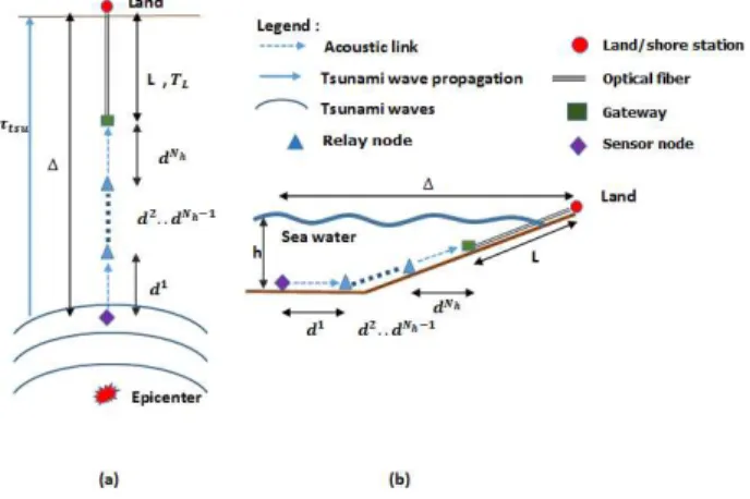
A relay sensor consists of an acoustic communication module, which is capable of transmitting and receiving data. Acoustic links operate in half-duplex communication mode. Linked together, they provide a multi-hop communication from the bottom pressure sensor to the optic fiber communication link. An undersea gateway node, attached to the fiber optic cable, is required to convert the received acoustic signal into an optical signal. The received information is forwarded to the control station ashore, for tsunami detection warning dissemination. Fig 1 illustrates the infrastructure.
The proposed system must deliver information reliably and in a timely manner, in order to meet the tsunami preparedness and response requirements. Furthermore, the infrastructure cost must be minimized in order to achieve deployment at scale. To this end, the system design must address two critical constraints, namely reliability and timeliness. The reliability constraint specifies that the data loss probability should not exceed a target threshold. Note that to send data over acoustic link reliably, the acoustic signal must be interpretable at the receiving node. This imposes a limit on the maximum distance between any two adjacent sensor nodes in the hybrid infrastructure. The timeliness constraint sets an upper bound on the delay of a message from the pressure sensor to the onshore station. This is necessary to deliver the tsunami warning on time for the disaster response managers to organize the evacuation plan.
Fig. 1: The topology for notational convention
node. Consequently, the need to accurately compute the acous-tic transmission loss becomes criacous-tical in order to meet the two main constraints of the the proposed optimization framework. To this end, we use Bellhop propagation model to determine acoustic transmission loss. We further incorporate the sea floor and underwater sound speed profiles to take into consideration the characteristic of the environment.
III. OPTIMIZATIONFRAMEWORKFORMULATION Figures 1(a) and 1(b) depict the proposed architecture viewed from the top and the side perspective, respectively. The legend of notations used in Fig. 1 is provided in table I.
The optimization framework is formulated as a minimization of infrastructure cost subject to the timeliness and reliability constraints. LetCtot, which depends onNh,∆, andd, denotes
the implementation cost. The minimization problem can be stated as follows:
M inimize Ctot(∆,d) =CF(∆,d) +CS(Nh)
Subject to
TW arn(∆,d)≥ΘT (1)
Ri(∆,d)≥ΘR; i= 1,2, ..Nh, (2) RF(∆,d)≥Θ
R (3)
L= ∆−
Nh X
i=1
di≥Lmin; (4)
∆≤∆max (5)
where d = {di|di > 0,1 ≤ i ≤ Nh}. The timeliness and
reliability requirements are represented by Eq. (1), Eq. (2), and Eq. (3), respectively.
In practice, a submarine fiber optic cable is used to connect the last undersea acoustic link to the central station onshore via an optic fiber gateway attached to the fore front of the cable. As the transmission over acoustic links approaches coastal area, the sea depth becomes shallower, thereby impeding transmission between sensor nodes. Furthermore, there may be a requirement that a minimum length of the fiber optic
to be deployed offshore be buried underneath the sea floor. This requirement is usually imposed by local government regulations in order to avoid cable damage due to ship’s anchor drop-off around coastal areas. To meet this requirement, an auxiliary constraint on the length of the fiber, L , must be added. This constraint is expressed in Eq. (4). The Eq. (5) expresses the fact that the distance of the pressure sensor from the onshore station should not exceed the epicenter. In the context of near-field tsunami, the value of ∆max obviously
doesn’t exceed the distance defined for near-field tsunami origin.
Because of the environment variability, in terms of sea floor profile and ambient noise characteristics, sensor nodes may not be equidistant. Therefore, the total number of the undersea nodes,Nh, which depends on the cost trade-off between optic
fiber and sensor nodes, cannot be determined a priori. A similar observation can be made with respect to Eq. (4), as PNh
i=1di
cannot simplify intoNh·d, which would have been the case if
all sensor nodes were equidistant. The variability ofNhfurther
compounds the complexity of the optimization problem. In the following, we introduce the cost model used in this optimization problem and elaborate on the timeliness constraint. We then derive the data delivery time and the link reliability.
A. Total Cost Formulation
In this framework, a linear cost function is used. Based on this function, the total cost, C, to deploy Q units, can be expressed as C = φQ+C0, where φ is the unit cost and
C0 is the initial cost. It is worth noting, however, that the
framework does not depend on a specific cost function. Other functions such as power-law and logarithmic could have been used.
TABLE I: Notation explanation
Notation Remark
Ctot Total deployment cost
CF Cost to deploy fiber
L Length of fiber
Lmin Minimum fiber optic length
∆ The distance of the pressure sensor node CS Cost to build undersea nodes
Nh Total number of undersea nodes, which also represent
the total number of acoustic links di The length of the i-th acoustic link
ΘT Expected time constraint ΘR Link reliability constraint
B. The Timeliness Constraint
The timeliness constraint function, TW arn(), can be
ex-pressed as follows:
TW arn(∆,d) =τtsu(∆)−τnet(∆,d)≥ΘT (6)
where τtsu() is the tsunami travel time over∆ andτnet() is
station ashore. Since fiber optic link is reliable and fast, the acoustic links bear the highest portion of the data delivery time.
Eq. (6) imposes a minimum distance of the pressure sensor node for a given ΘT. This minimum distance, denoted as
∆min, can be derived if the data delivery time of the proposed
infrastructure is made practically negligible. This would be possible if all-fiber deployment is chosen to cover ∆min.
This solution is considered as the most expensive solution. If either the epicenter or the pressure sensor distance is less than∆min, then Eq 1 will never be satisfied. In our heuristic
approach algorithm, ∆min holds important role for initial
feasible solution.
1) The Data Delivery Time : This quantity is dictated by transmission delay, propagation delay, processing delay and retransmissions due to packet error. A less reliable link requires more time to complete a successful data delivery. Hence, we need to take the link reliability constraint function into account. Since the reliability constraint function implies a probabilistic type of quantity, the data delivery time, τnet(), is calculated
as an average.
If TF()represents the average of data delivery time in the
fiber optic link andTS()represent the average of data delivery
time in the acoustic links, then the total data delivery time τnet()is expressed as follow:
τnet(∆,d) =TF(∆,d) +TS(∆,d) (7)
2) Tsunami Travel Time: To obtain tsunami travel time over ∆, tsunami propagation speed needs to be determined. However, tsunami propagation speed is dictated by the sea depth. Given a sea depth of h, the tsunami speed, vtsu, can
be derived from vtsu =
√
g·h, whereg is the gravitational acceleration. To approximate tsunami travel time by taking the variation of sea depth into account, the pressure sensor distance
∆ is divided intoKsmall intervals. The tsunami propagation speed in each interval is assumed to remain constant. Eq. (8) expresses the overall tsunami travel time as the sum of the travel time over K intervals, where xj and vj
tsu denote
the length and the tsunami propagation speed at j-th interval. Indeed, larger K results in more accurate result.
τtsu = K
X
j=1
xj
vtsuj (8)
C. The Reliability Constraint
The reliability constraint measures the probability of a successful data transmission. Given the data length of m, the probability of error-free received data at receiving node, R(), can be expressed as follows:
R(∆,d) = 1−BERr(∆,d)m (9)
where BERr is the probability of bit error. Since the fiber
optic link offers very high reliability, the discussion focuses on the acoustic link reliability constraints expressed in Eq. (2). To obtain the bit error probability over an acoustic link i, a probability distribution function F(p) is specified. This
probability distribution function represents the bit error char-acteristic in undersea environment. The probability function
F(p) also depends on the modulation scheme. In section V, we will specify F(p)in more detail.
To apply this function, we use p= Ebi
Ni
0 for the parameter. TheEi
bandN0idenote the energy per bit and equivalent white
noise on acoustic link i. The following equation:
Ebi= 1 rs ·
Pti·Ai(∆,d, f) (10)
provides the formulation to obtain the energy per bit on link i, wherePi
t,Ai(),f andrsrepresent the node’s transmission
power, the acoustic channel loss, the acoustic wave frequency and the sensor transmission rate at link i, respectively.
To approximate the equivalent white noise energy, Ni
0, Eq.
(11) is used. The equation divides the total noise power in the receiving node, W(f, B), with the receiver’s bandwidthB.
N0i = 1
B ·W(f, B) (11)
1) Acoustic Channel Loss: Acoustic channel loss is cal-culated as the total transmission loss inflicted by two main factors, namely spreading and absorption loss. A spreading loss is a signal attenuation as the acoustic signal travels further from the source, whereas the absorption loss is caused by the acoustic energy absorption as it traverses within sea water [10]. The acoustic energy absorption loss factor, denoted asa(f), is frequency dependent. This paper incorporates this absorption loss into Bellhop model in order to increase the accuracy of the channel loss computation.
To quantify the absorption loss, a(f), an empirical model, called as Thorp [11], is expressed as follows (in dB) :
a(f) = 0.11f 2
1 +f2 +
44f2
4100 +f2 + 2.75·10
−4f2+ 0.003
where f is in KHz. The equation above is still sufficiently valid for frequency above few hundreds of Hz.
2) Sea Background Noise: Sea background noise, sometime is referred to as sea ambient noise, is inherent acoustic fields that may interfere the acoustic channel. Their characteristics and intensities are location-specific. Based on their sources, the ambient noise main contributors can be grouped as follows: water motion, including also the effects of surf, rain, hail and tides, man-made sources, including ship activity and marine life [8]. Each contributor causes a frequency-dependent impact to the acoustic channel. The ambient noise also increases in shallower depth.
A number of ambient noise studies and measurements have been made since 1945 in deep-water and open ocean areas [8]. The ambient noise spectra then are summarized and presented in a group of curves [8], [12] as shown in figure 2. Fig. 2 is also known as Wenz curve.
To obtain the total noise powerW(f, B)at the receiver with the receiving bandwidth ofB Hz, the following equation,
W(f, B) =
Z
B
Fig. 2: Wenz curve, based on the work by [8]. This figure is taken from [12]
can be used. The termw(f)represents the sea ambient noise spectrum function.
3) Bellhop Propagation Model: Underwater acoustic wave is a propagating mechanical wave that is created by the alternating compression and dilations of the medium [12]. The compression and the dilations result from the dynamic changes of medium pressure. Bellhop propagation model is a finite element approach which is based on ray tracing model. Although ray tracing model has coarser accuracy than other models such as Normal Mode or Parabolic Equation, it tends to improve in high frequency, especially above 1 KHz [7].
Ray tracing model uses Helmholtz equation as the basis for derivation. If x = (x, y, z) denotes a point position
expressed in Cartesian coordinate, then Helmholtz equation can be written as follow:
∇2p+ ω 2
c2(x)p=−δ(x−x0) (13)
In underwater context, the termprepresents a function that quantifies the dynamic of medium pressure. The termc(x)is
the sound speed and ω is the angular frequency of the source located at x0. The solution of this equation results in two
equations, called as eikonalequation andtransport equations.
Eikonal equation is used to compute the travel time along the ray, whiletransport equation is used to compute transmission loss.
Bellhop model describes the acoustic wave as a bundle of acoustic rays emitting from a source within a range of depar-ture angles. Each acoustic ray will be computed independently. On their way to the receiver, acoustic rays may be reflected by either bottom, surface, or both. They may suffer from losses when being reflected by these boundaries. In addition to the reflection, the acoustic rays may also be refracted due
to different sound speed across sea water depth. Under these circumstances, each ray’s path is no longer in a straight line of trajectory and may differ one another.
Since each acoustic ray imposes a distinct path, they may result in different intensity and arrival time to each other at the receiving node. Therefore, transmission loss at the receiving node is calculated as the cumulative resultant of ray’s intensity. A Bellhop program is used [13] to compute propagation loss and acoustic travel time between two nodes separated by the distanced. To run the program, undersea sound speed and sea floor profiles need to be supplied.
4) Undersea Sound Propagation Speed: Undersea sound speed depends on temperature, water salinity and the water pressure. Some empirical models explained in [14] express the underwater sound speed as the function of these three variables. One of those is formulated by Mackenzie as follow :
vac= 1448.96 + 4.591T−(5.304e−2)T2+ (2.374e−4)T3
+1.340(S−35) + (1.630e−2)h+ (1.675e−7)h2 −(1.025e−2)T(S−35)−(7.139e−13)T h3 (14)
where T is the sea water temperature at the depth hand the salinity S. The temperature is measured in Celsius, the depth in meter, and the salinity in ppt (parts per thousand).
IV. THEHEURISTICAPPROACH FOROPTIMALSOLUTION Because the number of undersea sensors, Nh, is unknown
a priori, we propose a heuristic approach. The heuristic starts with an initial feasible solution. We consider an all fiber optic of maximum length∆minas the initial feasible solution of the
optimization framework. Note, however, that such a solution is also the most expensive. Subsequently, the use of additional sensors, which results in the reduction of optic cable length, is explored to determine if the overall cost can be reduced. More specifically, the heuristic reduces the length of fiber optic by a certain amount and augments the infrastructure with acoustic sensors. The length of the removed fiber depends on the constraint imposed on the distance between the new acoustic sensor and the optic gateway. The timing constraint is also checked upon the removal of the fiber optic. This process continuous until the heuristic converges to a least-cost, constraint satisfying topology.
The approach has two ways of adding new undersea sensors, namely inbound and outbound. An inbound procedure can be seen as a direct substitution for the reduced fiber optic. The term “inbound” is given because the replacement progresses toward the shore. A maximization problem is solved to find the optimal inbound acoustic link length, denoted as dib, subject
to the reliability and the timeliness constraints, ΘR and ΘT,
respectively. This process continuous until one of the the constraint is violated.
Data: Undersea sound speed and sea floor profile Result:L,d,Ctot,Nh
Compute max fiber optic length L0
= ∆min; Set i, j, k= 1;C0
tot,C
0
opt1,C 0
opt2,C 0
opt3=inf ;
while ∆j<∆maxandLj> Lmin do
Reduce fiber by replacing it with inbound linkdi ib
di
ib= maxdi S.T R(di)≥ΘR ; Update Lj; Increase i=i+ 1; ComputeTW arnj andCoptj 1 ;
while TW arnj <ΘT and∆j<∆max do
Reducediib (or extend fiber) by binary searching; Calculate the cost Coptj 2 ;
end Keep di
ib= maxdi S.T ΘR ;
while TW arnj <ΘT and∆j<∆max do Add outbound link dk
ob as
dk
ob= maxd
k S.T R(do)≥Θ
R ; Update ∆j; Increase k=k+ 1 ; ComputeTW arnj and the cost Coptj 3
end
DefineCjtot =min{Coptj 1, C
j opt2, C
j opt3};
if Ctotj ≥C j−1
tot or∆j≥∆maxorLj≤Lmin then
Ctotj =Cj−1
tot ;Lj=Lj−
1 ;
Break ; Increasej=j+ 1; end
L=Lj ,d={(dib,dob)},dib={dnib|1< n < i}; dob={dnob|1< n < k},Nh=i+k,Ctot=Ctotj ;
Fig. 3: Heuristic Approach
Fig. 4: Illustration of our heuristic approach
the latest added inbound link. The second technique adds one or more “outbound” acoustic links toward the tsunami origin. A maximization problem is then solved to find the optimal outbound acoustic link length, dob, subject to the reliability
and the timeliness constraint.
The addition of an inbound link and possibly outbound links counts for one cycle. The cycle will be repeated if the implementation cost computed from the previous cycle
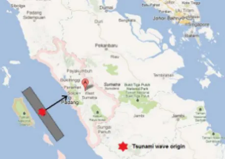
Fig. 5: Location of Padang, West Sumatra, Indonesia
TABLE II: Constants and Design Parameters
Parameter Value Remark
Tx Power Node 40 Watt
Modulation Binary Freq. Shift Keying Data Link protocol Stop and Wait Lmin 10 Km
∆max 90 Km
w(f)(1) 110−20 log10 f
10 Calm, in dB reµ P a 2
/Hz w(f)(2) 125−20 log10
f
10 Moderate, in dB reµ P a 2
/Hz w(f)(3) 130−20 log10
f
10 Severe, in dB reµ P a 2
/Hz m 120 bits Packet length
rf 200 Mbps Fiber transmission rate
γ 0.2 See section V-G2
ΘT {15,16,. . .,20}
ΘR {0.75, 0.775,. . ., 0.99, 0.995, 0.999}
Some time is written in %, i.e 0.75=75%
rs {40, 80,. . .,440, 480, 520} in bit per second (bps)
f {4, 6, 8,. . ., 26 28 30} in KHz
is more expensive than the subsequent one. Otherwise, the approach will stop and returns the final result. These cycles may either eliminate completely the fiber optic or reach an infinite detection distance, ∆. Given the fact that Lmin and
∆max exist, the heuristic will stop whenever one of these
boundaries is reached. Figure 3 and 4 illustrate our heuristic approach.
V. CASESTUDY
The main objective of the case study to derive an “optimal” configuration of a hybrid infrastructure for Padang City, West Sumatra, Indonesia, based on the developed framework. The framework will be applied under different sea environmental factors and design parameters. The region under consideration is shown in Fig. 5. The gray box in the figure represents the area of possible epicenters or tsunami origins. The underwater nodes and fiber optic would be deployed along the line pointing to the coast. The sea floor and the underwater sound speed profile data collected by [15] are used with permission. Different environment factors that impact background noise are also considered.
A. Constants and Design Parameters
levels of ambient noise spectrum are assumed, namely calm, moderate, and severe. These assumptions reflect the wind-generated noise and associate them to the sea states scale as depicted in Wenz curve [12]. A ”calm” assumption is associated to the sea state of 0.5. In this state, the noise is created by a calm sea with waves reaching up to 0.1 meter in average. A ”moderate” level is referred to as the noise induced by the sea with sea state of 4. At this level, the waves may reach a height of 3 meter in average. The highest noise level is attained when the sea is in ”severe” state, which is caused by the wind that brings the sea waves up to 7 meters height. This state represents a sea scale of 6 in Wenz curve. In our case study, the underwater sensor transmits pressure data with some attributes, including the date, time, and battery status. We consider a 120 bit frame length to be sufficient to accommodate these data, including the frame overhead. We also assume that no forward error correction scheme is applied.
To deal with different ambient noise levels, this paper defines three design parameters, namely the link reliability constraint, acoustic carrier frequency and underwater transmis-sion rate. This paper derives the optimal configuration and the implementation cost with these design parameters varied and analyze the results under different ambient noise conditions.
B. Cost Function Assumption
To limit the scope of analysis, the case study only focuses on linear cost function. Our discussion associates the variableQto two independent quantities. They mainly represent the physical attributes with respect to the infrastructure’s component. More specifically, the fiber optic implementation cost is governed by the length of fiber opticLand the fiber optic transmission rate rf, whereas the underwater sensor network cost is dictated by
the number of nodes Nh and the node’s transmission rate rs.
The following two equations express the cost function for the fiber optic and the undersea sensor network, respectively.
CF =φf·rf·L
CS=φs·rs·Nh (15)
To carry the cost analysis, the unit cost of sensor φs is
normalized to the fiber optic unit costφf such thatφs=γφf.
The total cost,Ctot, is expressed as the ratio of the cost of the
most expensive solution. Without loss of generality, we assume that the initial deployment cost of the fiber optic and undersea sensors are the same.
C. Formulation for Data Delivery Time
Both the fiber optic and multi-hop acoustic links use auto-matic repeat request (ARQ) as the retransmission scheme. A stop and wait ARQ will be implemented in a per-hop basis. Consequently, the round trip transmission time of a packet and its associated acknowledgment can be expressed as follows:
trt(d) =tm+ 2tp(d) +ta
The parameter tm represents the data transmission time,
tp(d) the acoustic propagation time traversing through a link
of length d and ta the acknowledgment packet transmission
time. Given the reliability function,R(∆,d), the average delay
Fig. 6: Courtesy of BPPT [15]: Underwater Sound Speed around of our case study area
to transmit a packet and receive its acknowledgment can be expressed as follows:
T = 1
R(∆,d)·trt(d) (16)
Eq. (16) is applicable for both fiber optic and acoustic links. Based on Eq. (7), we can deduce a formulation for total data delivery time, τnet(), as follows :
τnet(∆,d) =
tF rt(L)
RF(∆,d)+
Nh X
i=1
tS rt(di)
Ri(∆,d) (17)
In the above equation, tF
rt denotes the round trip time
transmission in the fiber optic link andtS
rt(di)is the round trip
time transmission in acoustic linki. In the proposed heuristic, Eq. (17) is invoked each time the timeliness constraint is verified with a new value of Nh being assigned for each
invocation. In this paper, the fiber optic reliability is considered hight, i.e. RF ≈1. Thus, the data delivery time in fiber optic
link, TF is approximately equal totF rt.
D. Assumption on Bit Error Probability Distribution Function
The case study uses binary frequency shift keying (BFSK) for the modulation scheme. To calculate bit error probability, this paper adopts the probability distribution function formu-lated in [16]. Let Eib
Ni
0
be the ratio of bit energy to equivalent white noise at link i. The bit error probability at linkican be expressed as follows:
BERi
r(∆,d) =
v Γ(v)
Z ∞
0
uv−1
2v+uE
i b
Ni
0
du (18)
In the above equation,Γ()represents the Gamma function, with u = y2, where y is the real part of complex value of
signal amplitude random variable.
E. Underwater Sound Speed and Sea Floor profile
Fig. 7: Sea depth profile at area of interest
Fig. 8: Propagation path, generated using the Bellhop model
F. Acoustic Propagation Path and Transmission Loss
The varying underwater sound speed, combined with the sea floor profile, determines the propagation path of the acoustic wave. Fig. 8 shows the acoustic wave propagation generated using the Bellhop model, represented in 10 rays in total with departure angle of 10 degrees. The acoustic wave is emitted from a 40 km offshore-source with a frequency of 4 KHz. Due to the variation of undersea sound speed, the acoustic rays follow the paths depicted in Fig. 8. Fig. 9 illustrates the channel loss characteristics when two different acoustic carriers, with frequencies, 4 KHz and 18 KHz, are emitted from two different locations. It can be observed that even when the acoustic waves are transmitted from the same distance, the acoustic waves with different frequencies and locations may produce different channel loss characteristics.
G. Results
1) Minimum Sensor Distance ∆min: Given a set of values
of the warning time,ΘT, listed in table II, the corresponding
set of∆min is determined based on the sea floor profile data,
using the equations described in section III-B1 and III-B2. These values represent the initial solutions of the proposed heuristic and are listed in table III.
TABLE III: List of∆min
ΘT
(minutes) 15 16 17 18 19 20
∆min(Km) 23.6 25.2 27.1 29.2 31.9 35.5
Fig. 9: Channel loss characteristics
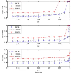
Fig. 10: Total cost for various reliability for 3 different frequencies withΘT = 20minutes
2) The Results under Different Reliability Constraints: The focus is on investigating how the cost optimality can be achieved for different reliability constraints, frequencies and environmental factors. Three different acoustic wave frequen-cies, 6, 18 and 30 KHz are selected to represent the low, middle and high frequency regions, respectively. In this case, we set ΘT equals to 20 minutes and maintain the sensor’s
transmission rate at 120 bps. The remaining constants and parameters used in this experiment are listed in table II. The results are depicted by Fig. 10. The three sub figures, Fig 9(a), 9(b) and 9(c) show the results for severe, moderate and calm environments, respectively.
The results show that the optimal cost of the infrastructure does not increase significantly when the reliability constraint does not exceed 0.925. Consequently, if the desired reliability does not exceed 0.925, a low-cost hybrid infrastructure using a low region of frequencies, is feasible. Achieving higher reli-ability, however, gives rise to trade-offs between the frequency used and the noise environment.
Fig. 11: Total cost for various frequency with ΘR= 0.99
6 KHz frequency results in low-cost infrastructure in a calm environment, using a frequency of 18 KHz achieves minimum cost, Ctot, of approximately 2.93% less than the cost of an
infrastructure operating with 6 KHz in moderate environment. The difference becomes more notable for higher reliability re-quirements in severe environment. Rather than using undersea sensors operating with a frequency of 6 KHz, the optimization framework identifies the 18-KHz-based infrastructure a more cost-efficient infrastructure to achieve. The findings provide the basis to determine an optimal carrier frequency for different ambient noise levels. These findings will be discussed in detail in the following section.
3) The Results under Different Carrying Frequencies f:
Based on the findings observed in the previous section, a case analysis under different acoustic carrier frequencies and environment factors is the subject of this section. To this end, a reliability constraint of 0.99 is selected while retaining the timeliness constraint at 20 minutes. Fig. 11 shows the results of this study.
The result confirms the findings in section V-G2. Each ambient noise level imposes an optimal frequency range to use in order to achieve the minimum cost. In a calm environment, the optimal cost is achieved for low-range frequencies, namely 6 to 12 KHz. The frequency range shifts to a higher region as the environment becomes noisier.
In moderate environments, the optimal infrastructure cost is achieved for a frequency range of 10 to 16 KHz, whereas in severe environments, the frequencies to achieve optimal cost range from 12 to 18 KHz. Based on these results, an optimal-cost infrastructure to meet the reliability and timeliness con-straints in the three different environments can be achieved using a carrier frequency of 12 KHz. For our case study, the minimum cost infrastructure requires 4, 7 and 9 nodes to be deployed for calm, moderate and severe environments, respectively. Table IV lists, for each environment, the distance, di, betweeen two consecutive undersea sensors and the length
of the optic fiber associated with the configuration.
4) The Results under Different Sensor Tx Rates rs: This
section focuses on investigating the impact to the results due to different undersea node’s transmission rates. A frequency of 12 KHz, 20 minutes for the time constraint and 0.99 for the
Fig. 12: Total cost for various node transmission rate under 3 different environments, withΘR= 0.99
TABLE IV: Optimal configuration at frequency of 12 KHz
Noise Acoustic Link Length (Km) L
(Km)
d1 d2
d3 d4
d5 d6
d7 d8
d9 Calm 8.23 8.60 8.85 8.04 - - - -
-Moderate 3.08 3.85 4.19 4.10 5.18 4.68 3.49 - - 10
Severe 1.54 2.50 2.57 3.02 3.09 3.36 3.35 3.13 3.38 11.1
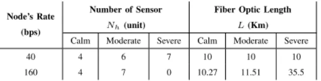
TABLE V: Optimal configuration with node’s rate of 40 bps and 160 bps
Node’s Rate
(bps)
Number of Sensor
Nh(unit)
Fiber Optic Length
L(Km)
Calm Moderate Severe Calm Moderate Severe 40 4 6 7 10 10 10 160 4 7 0 10.27 11.51 35.5
reliability constraint are used. The result is show in Fig. 12. A higher transmission rate requires a shorter acoustic link length to achieve the expected reliability. The cost increases exponentially and becomes more significant in severe noise environments. Table V shows the optimal results for the transmission rates of 40 and 160 bps. A 40 bps transmission rate doesn’t incur significant increase in total cost when the environment becomes noisier. The cost increase is contributed by the number of undersea sensors. A more significant cost increase is observed for higher transmission rates. As the noise becomes worse, the cost increase is contributed by both the need of extra underwater sensors and the extension of the fiber optic cable. These results suggest that lower transmission rates is less sensitive to the impact of different ambient noises. However, selecting a very low transmission rate may violate the application data delivery time constraint, especially when larger amount of data are to be sent.
VI. CONCLUSION ANDFUTUREWORK
the Indian Ocean. Lessons learned from previous tsunamis reveal that a reliable and timely warning system increases the community resilience to tsunami disaster. To this end, we develop an optimization framework, which is used to derive a feasible and cost-effective infrastructure for NFT detection and warning. A case study is used to demonstrate the proposed approach and derive a feasible infrastructure for a region, which is prone to NFT, namely Padang City, West Sumatra, Indonesia. The results show that the proposed approach can lead to the derivation of an infrastructure that can guarantee 20 minute warning time and 99%data communication reliability. The proposed framework can be used to provide insights and guidance related to the development and deployment of undersea tsunami detection and warning systems. As future work, the model can further be enhanced by incorporating multi-path loss models for a more realistic communication model and the development of energy management strategies to extend the lifetime of the undersea sensor subnetwork.
ACKNOWLEDGMENT
This material is based in part upon work supported by the National Science Foundation under Grants Number OCE 1331463: Hazards SEES Type 2: From Sensors to Tweeters: A Sustainable Socio-technical Approach for Detecting, Mit-igating, and Building Resilience to Hazards. Any opinions, findings, and conclusions or recommendations expressed in this material are those of the authors and do not necessarily reflect the views of the National Science Foundation
REFERENCES
[1] UNESCO-IOC, “Tsunami glossary, 2008,”IOC Technical Series, Paris, France, vol. 85, 2008.
[2] E. Sasorova, M. Korovin, V. Morozov, and P. Savochkin, “On the Prob-lem of Local Tsunamis and Possibilities of Their Warning,”Oceanology 2008, Pleiades Publishing Inc, vol. 48, no. 8, pp. 634–645, 2008. [3] “NDBC- deep-ocean assessment and reporting of tsunamis (DART)
description,”[online] http://www.ndbc.noaa.gov/dart/dart.shtml, visited on April 2014.
[4] L. Comfort, T. Znati, M. Voortman, Xerandy, and L. Freitag, “Early detection of near-field tsunamis using underwater sensor networks.”
Science of Tsunami Hazards, vol. 31, no. 4, 2012.
[5] C. Teng, S. Cucullu, S. M. Arthur, C. Kohler, B. Burnett, and L. Bernard, “Buoy vandalism by noaa national data buoy center,”NOAA National Data Buoy Center1 University of Southern Mississippi2 report, June 2010.
[6] G. Schmitz, W. Rutzen, and W. Jokat, “Cable-based geophysical mea-surement and monitoring systems, new possibilities for tsunami early-warnings,” inUnderwater Technology and Workshop on Scientific Use of Submarine Cables and Related Technologies, 2007. Symposium on. IEEE, 2007, pp. 301–304.
[7] M. Porter and Y.-C. Liu, “Finite-element ray tracing,”Theoretical and Computational Acoustics, World Scientific Publishing Co, vol. 2, 1994. [8] G. M. Wenz, “Acoustic ambient noise in the ocean: Spectra and sources,” The Journal of the Acoustical Society of America, vol. 34, no. 12, pp. 1936–1956, 1962. [Online]. Available: http://scitation.aip.org/content/asa/journal/jasa/34/12/10.1121/1.1909155 [9] J. McCloskey, A. Antonioli, A. Piatanesi, K. Sieh, S. Steacy, S. S. Nalbant, M. Cocco, C. Giunchi, J. D. Huang, and P. Dunlop, “Near-field propagation of tsunamis from megathrust earthquakes,”
Geophysical Research Letters, vol. 34, no. 14, 2007. [Online]. Available: http://dx.doi.org/10.1029/2007GL030494
[10] F. B. Jensen, Computational Ocean Acoustics. Springer Science & Business Media, 1994.
[11] L. M. Brekhovskikh and I. Lysanov,Fundamentals of ocean acoustics. [12] C. Erbe, Underwater Acoustics: Noise and the Effects on Marine Mammals, a Pocket Handbook, 3rd ed. JASCO Applied Sciences, 2011.
[13] M. Porter, “The bellhop manual and userguide: Preliminary draft.” [Online]. Available: http://oalib.hlsresearch.com/Rays/HLS-2010-1.pdf [14] P. C. Etter, Underwater Acoustics Modeling and Simulation, 4th ed.
CRC Press, 2013.
[15] B. Balai Teknologi Survei Kelautan, “Baruna jaya bppt 2014.” [Online]. Available: http://barunajaya.bppt.go.id/index.php/en.html
[16] W.-B. Yang and T. C. Yang, “M-ary frequency shift keying communi-cations over an underwater acoustic channel: Performance comparison of data with models,”The Journal of the Acoustical Society of America, vol. 120, no. 5, pp. 2694–2701, 2006.
X. Xerandyreceived the Bachelor and Master de-gree from Bandung Institute of Technology, Indone-sia, majoring in Electrical Engineering in 2006. He joined as the researcher in Agency of Technology Assessment and Application (BPPT), Indonesia since 2008. Currently, he is enrolled as a PhD student in School of Information Science, University Pitts-burgh. His primary research is in telecommunication and networking. His current research project is to develop environment-aware undersea sensor network for tsunami disaster mitigation.
Taieb Znatiis Professor in the Department of Com-puter Science, with a joint appointment in ComCom-puter Engineering at the School of Engineering. He served as the Director of the Computer and Network Sys-tems Division at the National Science Foundation. He also served as a Senior Program Director for networking research at the National Science Foun-dation. In this capacity, He led the Information Technology Research Initiative, a cross-directorate research program. Dr. Znatis main research interests are in the design and analysis of evolvable, secure and resilient network architectures and protocols for wired and wireless communication networks. He is also interested in bio-inspired approaches to address complex computing and communications design issues that arise in large-scale heterogeneous wired and wireless networks. He is a recipient of several research grants from government agencies and from industry.
![Fig. 2: Wenz curve, based on the work by [8]. This figure is taken from [12]](https://thumb-eu.123doks.com/thumbv2/123dok_br/16315651.187140/5.918.144.382.92.407/fig-wenz-curve-based-work-figure-taken.webp)
![Fig. 6: Courtesy of BPPT [15]: Underwater Sound Speed around of our case study area](https://thumb-eu.123doks.com/thumbv2/123dok_br/16315651.187140/7.918.581.750.99.233/fig-courtesy-bppt-underwater-sound-speed-case-study.webp)