REM WORKING PAPER SERIES
Evaluating the European bank efficiency using Data
Envelopment Analysis: evidence in the aftermath of the recent
financial crisis
Cândida Ferreira
REM Working Paper 0109-2019
December 2019
REM – Research in Economics and Mathematics
Rua Miguel Lúpi 20,
1249-078 Lisboa,
Portugal
ISSN 2184-108X
Any opinions expressed are those of the authors and not those of REM. Short, up to two paragraphs can be cited provided that full credit is given to the authors.
1
Evaluating the European bank efficiency using Data Envelopment
Analysis: evidence in the aftermath of the recent financial crisis
Cândida Ferreira
ISEG, UL – Lisbon School of Economics and Management of the Universidade de Lisboa
UECE - Research Unit in Complexity and Economics
REM – Research in Economics and Mathematics
R. Miguel Lupi, 20, 1249-078 - LISBOA, PORTUGAL
e-mail: [email protected]
Financial support by FCT (Fundação para a Ciência e a Tecnologia), Portugal is gratefully
acknowledged. This article is part of the Strategic Project (UID/ECO/00436/2019).
Abstract
This paper seeks to contribute to the analysis of the bank efficiency in the European Union in the aftermath of the recent crisis, using Data Envelopment Analysis (DEA) and considering a sample of 485 banks from all current EU member-states between 2011 and 2017. The results obtained confirm the existence of bank inefficiency, and that this inefficiency is mostly due to inefficient managerial performance and bad combinations of the considered bank inputs and outputs. The results also provide enough evidence of appropriate scale production and dynamic technological changes during the considered interval. Moreover, the results obtained using panel estimates to explain the bank total factor productivity changes allow us to conclude that the choices of the banks in terms of the fixed assets, the profit before tax to the average assets, as well as the ratio of the off-balance sheet items to total assets contribute positively to the productivity changes. On the other side, the ratio of the impaired loans to equity, and the bank interest margins are not in line with the total factor productivity changes of the EU banking sector.
Keywords: EU banking sector; bank efficiency; Data Envelopment Analysis; Malmquist
Index
2
Evaluating the European bank efficiency using Data Envelopment
Analysis: evidence in the aftermath of the recent financial crisis
1. Introduction
The banking sector plays a recognised crucial social-economic role. Overall, banks are supposed to collect savings and to allocate resources in an efficient way. They are also supposed to manage risks and to help solving potential adverse selection and moral hazard problems caused by imperfect information between borrowers and lenders.
Recently, the banking institutions have been exposed to several challenges such as increased liberalisation, deregulation, technological changes and internationalisation. Under these conditions, banks have strong incentives to maximize high-valued investment opportunities, and sometimes they don’t prevent risks and contribute to financial distresses and insolvencies that can lead to financial crises.
In the European Union (EU) banks had to face not only the challenges and consequences of the recent international financial crisis but also some specific challenges, namely those related to the process of European integration, to the sovereign debt crisis, and to the crisis of the European Economic and Monetary Union (EMU) that affected most of the EU member-states.
These challenges raised questions related to the resilience and performance of the EU banking institutions particularly in the aftermath of the crises.
This paper aims to contribute to the strand of literature that analyse the European banking markets represented, among others, by Tanna et al (2011), Chortareas et al (2013), Asmild and Zhu (2016), Fujii et al. (2018).
Here a two-stage approach is adopted to address research questions related to the response of the EU banking institutions to the challenges of the different crises. We use Data Envelopment Analysis (DEA) techniques to measure and analyse the European bank efficiency between 2011 and 2017, considering a sample of 485 banks from all current EU member-states.
3 In the first stage, we consider the different concepts and measures of DEA bank efficiency, namely the technical, pure technical and scale efficiency; the allocative and cost efficiency; as well as the technical, technological, pure technical, scale efficiency changes and the total factor productivity change provided by the Malmquist indices. In the second stage, we use panel random effects estimates to analyse the influence of some bank performance indicators and production conditions to explain the total factor productivity changes.
Overall, our results confirm the existence of bank inefficiency, and that this inefficiency is mostly due to inefficient managerial performance and bad combinations of the considered bank inputs and outputs. The results also provide enough evidence of appropriate scale production and dynamic technological changes during the considered interval.
Moreover, the results obtained in the second stage allow us to conclude that the choices of the banks in terms of the fixed assets, the profit before tax to the average assets, as well as the ratio of the off-balance sheet items to total assets contribute positively to the EU bank total factor productivity changes. On the other side, the ratio of the impaired loans to equity, and the bank interest margins are not in line with these productivity changes.
The paper is organized as follows: Section 2 presents the literature review; the methodology is presented in Section 3; Section 4 provides information about the data, reports and discusses the results obtained; Section 5 concludes.
2. Literature review
The analyses on efficiency mostly follow the pioneer contribution of Farrell (1957) considering the possibility of using the available data of the firms’ inputs and outputs to define the efficiency frontier as the best combination of these inputs and outputs, measuring the firms’ efficiency with the deviations from the defined efficiency frontier (Coelli, 1996; Sherman and Zhu, 2006; 2013).
4 During the last few decades the efficiency of financial institutions has been widely studied, analysing the banks’ ability to produce output with minimal resources or input, commonly considering the ratio of the banks’ outputs over the inputs (Cooper et al, 2006; Chen et al, 2008). The efficiency production frontiers can be obtained with parametric and non-parametric approaches.
The Stochastic Frontier Analysis (SFA), is a parametric approach, following the methodology that was first proposed by Aigner et al (1977) and later developed by Battese and Coelli (1988, 1995). SFA is based on a problem of economic optimisation, more precisely, on the maximisation of profits or the minimisation of costs, given the assumption of a stochastic optimal frontier. Several studies used SFA to analyse the efficiency of the European banks. For example, Lozano-Vivas et al (2011) conclude that there is cost efficiency improvement of merger processes and consolidations in Europe from 1998 to 2004. Aiello and Bonanno (2013) use SFA to evaluate the cost and the profit efficiency of the Italian banking sector over the years 2006-2011 stating that, overall, the Italian banks performed well during the considered period, despite the high heterogeneity in the results obtained. Vozková and Kuc (2017) consider a sample of 649 European cooperative banks and use SFA to analyse the recent trends in bank cost efficiency concluding that the average inefficiency of European cooperative banks is increasing since 2008. Kuc (2018) also employs the SFA on a set of 183 cooperative banks from 12 European countries during the 2006-2015 period, revealing that smaller European cooperative banks are significantly more cost efficient than the bigger ones. Oliveira (2017) uses SFA to measure the efficiency of 122 European banks from a group of 15 EU member-states for the 2000−2013 period and find that in 2013 the median European bank operated with costs 25 to 100% above the efficient level; and also that the inefficiency of financial intermediation has been increasing over time, possibly driven by the least efficient banks.
Bank efficiency has also been analysed with non-parametric approaches, namely with the Data Envelopment Analysis (DEA) that was first developed by Charnes et al (1978) and developed among others by Ali and Seiford (1993), Lovell (1993), Charnes et al (1994), Cooper et al (2006). DEA is nowadays a well-tested non-parametric efficiency approach, based on a linear
5 programming methodology that is appropriate to measure the efficiency of different decision-making units (DMUs) using multiple inputs and outputs in a production process. Ultimately DEA has become also a method of performance evaluation and benchmarking against best-practice (Cook et al 2014). DEA techniques have been used often to assess and compare the efficiency performance of banks in different countries or regions (Annex 1 presents some recent examples of studies on DEA bank efficiency).
DEA has also been used to analyse the performance of the European banking institutions, both in single focussed studies and in multi-country focussed studies.
Examples of single focussed DEA studies include Favero and Papi (1995) which provide measures of the technical and scale efficiencies in the Italian banking industries by implementing non-parametric DEA on a cross section of 174 Italian banks taken in 1991. The conclusions point to the existence of both technical and allocative efficiency; in addition, when a regression analysis is used, bank efficiency is best explained by productive specialization, size and, to a lesser extent, by location.
Drake (2001) analyses relative efficiencies within the banking sector and the productivity change in the main UK banks over the period 1984 to 1995. The results obtained provide important insights into the size-efficiency relationship in the considered sample of banks and offer a perspective on the evolving structure and competitive environment within which the banks are currently operating. Webb (2003) utilizes DEA window analysis, to measure the relative efficiency levels of large UK retail banks during the period 1982-1995, mostly finding that the overall long run average efficiency trend is falling, and also that all banks in the study show reducing levels of efficiency over the entire time period.
Tanna et al (2011) consider a sample of 17 banking institutions operating in the UK between 2001 and 2006 and use DEA techniques to provide empirical evidence on the association between the efficiency of UK banks and board structure, namely board size and composition. They find some evidence of a positive association between board size and efficiency as well as robust evidence that board composition has a significant and positive impact on all measures of efficiency.
6 More recently, Ouenniche and Carrales (2018) also assess the efficiency profiles of UK banks, collecting data from 109 commercial banks over the years 1987-2015, and conclude that, on average, commercial banks operating in the UK are yet to achieve acceptable levels of overall technical efficiency, pure technical efficiency, and scale efficiency.
Examples of multi-country DEA studies analysing the efficiency of the European banks include Casu and Molyneux (2003) investigating the existence of improvement in and convergence of productive efficiency across European banking markets in the aftermath of the creation of the Single Internal Market with efficiency measures derived from DEA estimations. Overall, the results suggest that there was a small improvement in the bank efficiency levels, although there was not enough evidence to support the convergence of the EU banks’ productive efficiency. Chortareas et al (2013) consider a large sample of commercial banks operating in 27 European Union member states over the 2000s to estimate bank-specific efficiency scores with DEA. In particular, they investigate the dynamics between the financial freedom counterparts of the economic freedom index drawn from the Heritage Foundation database and bank efficiency levels. Their results suggest that the higher the degree of an economy’s financial freedom, the higher the benefits for banks in terms of cost advantages and overall efficiency. Moreover, the results also reveal that the effects of financial freedom on bank efficiency tend to be more pronounced in countries with freer political systems in which governments formulate and implement sound policies and higher quality governance.
Grigorian and Manole (2016) use DEA estimates based on data from 29 European countries, and measure the perception of sovereign risk and its impact on deposit dynamics over the period 2006-2011. The results obtained showed that the exposure of the banking sector to sovereign risk negatively affected the growth of consumer deposits over and above the impact of macroeconomic conditions. Moreover, the paper’s conclusions underline that during crisis times the perceived risks become more important than financial performance in determining the depositors’ choices. Tuskan and Stojanovic (2016) study the efficiency of the banking industry, for the period 2008– 2012 on a sample of 28 European banking systems, suggesting that, in general, banking systems in post-transition countries have a higher cost efficiency. At the same time, Asmild and Zhu
7 (2016) analyse the risk and efficiency of the European banks considering a sample of 71 banks from 20 different EU member-states for the years 2006-2009, analysing some potential bias and limitations of the DEA estimates and demonstrating that the decreases in efficiency scores after weight restrictions are significantly higher for the bailed-out banks than for the non- bailed-out banks.
Kocisova (2017) analyses revenue efficiency of the banking sectors in the European Union countries in 2015 and mostly concluded that the large banking sectors appear to be most efficient. Degl'Innocenti et al (2017) use a two-stage DEA model to analyse the efficiency of 116 banks from nine Central and Eastern European (CEE) countries, members of the EU, covering the period 2004-2015. Overall, the results obtained indicate a low level of efficiency over the entire period of analysis, especially for Eastern European and Balkan countries.
San-Jose et al (2018) study the relationship between economic efficiency and sustainability of banking in Europe applying DEA techniques to a sample of 2752 financial institutions from EU-15 countries in 2014. They mostly conclude that there is no single model of social and economic efficiency according to the type of financial entity in Europe as there is evidence of different behaviours in different European countries.
3. Methodology
Data Envelopment Analysis (DEA) was first developed by Charnes et al (1978) and developed among others by Ali and Seiford (1993), Lovell (1993), Charnes et al (1994), Cooper et al (2006). Nowadays DEA is a well-tested non-parametric efficiency approach, based on a linear programming methodology that is appropriate to measure the efficiency of different decision-making units (DMUs) using multiple inputs and outputs in a production process. Ultimately DEA has become also a method of performance evaluation and benchmarking against best-practice (Cook et al 2014).
8 The model proposed by Charnes et al (1978) is based on the assumption of constant returns to scale and is very well presented in Coelli (1996) assuming that each of the considered N firms (or DMUs) use K inputs to produce M outputs, being X the KxN input matrix and Y the MxN output matrix that include the data of all the N DMUs. Using linear programming, one of the ways to measure the efficiency is by solving the problem:
Min, ,
Subject to: -yi + Y 0; yi - X 0; 0 (1)
(where is a scalar and is a Nx1 vector of constants).
Solving this problem, we obtain, for each DMU, the efficiency score . In all situations ≤ 1; when =1 the correspondent DMU is in the efficient frontier, and when they are not in the frontier
the values of 1– represent the distance to this frontier, or the measure of their technical
inefficiencies.
Under these conditions, the technical efficiency of each DMU is a comparative measure of how well it processes the inputs to obtain the desired outputs in comparison with the best achieved performance that is represented by the production possibility frontier. This overall efficiency measure depends not only on the input/output specific combination (representing the pure technical efficiency) but also on the scale of the production operation (or the scale efficiency). Still following Coelli (1996), we can introduce the assumption of variable returns to scale including the convexity constrain N1’ = 1 in model (1) and solving the following linear
programming problem to obtain the measure of the pure technical efficiency:
Min, ,
Subject to: -yi + Y 0; yi - X 0; N1’ = 1; 0 (2)
(where is a scalar, is a Nx1 vector of constants, and N1 is a Nx1 vector of ones).
Under the assumption of variable returns to scale the measure of (pure) technical efficiency basically captures the managerial performance. The scale efficiency represents the ability of the management to choose the scale of the production and can be obtained as the ratio of the overall
9 technical efficiency (under the assumption of constant returns to scale) and the pure technical efficiency (see, among others, Kumar and Gulati, 2008; Fujii et al, 2018).
In order to obtain the allocative efficiency, we first need to get the cost efficiency measure, solving the problem
Min,xi* wi ’ xi*,
Subject to: -yi + Y 0; xi * - X 0; N1’ = 1; 0 (3)
(where wi is a vector of the prices of the inputs of the i-th DMU, xi * is the cost-minimising vector
of the input quantities for the i-th DMU, given the input prices xi, and the output levels yi).
Solving this problem, we can obtain the value of the cost efficiency of the i-th DMU as the ratio of the minimum cost to the observed cost of this DMU, wi ’ xi*/ wi ’ xi. Moreover, and as well
demonstrated in Coelli (1996), the allocative efficiency (AE) is obtained as the ratio of the cost efficiency (CE) to the technical efficiency (TE), that is AE=CE/TE.
When considering panel data, we can also use a DEA linear programme to get a Malmquist index that measures the productivity change, decomposing it into the technical change and the technical efficiency change (see among others, Candemir et al, 2011) the Malmquist productivity change index between the period t and the period t+1 can then be defined as
𝑚(𝑦𝑡+1, 𝑥𝑡+1, 𝑦𝑡, 𝑥𝑡) = [ 𝑑𝑡(𝑥𝑡+1, 𝑦𝑡+1) 𝑑𝑡(𝑥 𝑡, 𝑦𝑡) ×𝑑 𝑡+1(𝑥 𝑡+1, 𝑦𝑡+1) 𝑑𝑡+1(𝑥 𝑡, 𝑦𝑡) ] 1/2 (𝟒)
This index can be decomposed into the Efficiency Change (EC) = 𝑑0
1+1 (𝑥1+1,𝑦1+1) 𝑑01 (𝑥1,𝑦1) (𝟓) and the Technical Change (TC) = [ 𝑑0𝑡(𝑥𝑡+1,𝑦𝑡+1) 𝑑1𝑡+1(𝑥 𝑡+1,𝑦𝑡+1)× 𝑑0𝑡(𝑥𝑡,𝑦𝑡) 𝑑1𝑡+1(𝑥 𝑡,𝑦𝑡)] 1/2 (𝟔)
Overall, it is generally recognised that DEA is an appropriate method to analyse and measure efficiency, including bank efficiency, and that in comparison with other tested methodologies, it presents some advantages, such as the possibility of handling with multiple inputs and outputs without and explicit definition of a production function, the possibility to be used with any
input-10 output measurement, and the possibility to obtain efficiency (and inefficiency) measures for every DMU.
On the other hand, DEA has also some recognised disadvantages, namely the fact that we cannot test for a better specification, as well as the fact that the results are very sensitive to the chosen inputs and outputs, as the number of efficient DMUs tend to increase with the inclusion of more input and output variables (see, for example, Ali and Lerme, 1997; Johnes, 2006; Berg, 2010).
In the second stage of our methodology, we use panel data estimates to analyse the influence of some bank-specific factors on the total factor productivity change, measured with one of the Malmquist indices.
Following, among others, Wooldridge (2010), we consider the general multiple linear panel regression model for the cross units (the DMUs) i = 1,…,N, which are observed for several time periods t =1,…,T:
𝑦
𝑖,𝑡= 𝛼 + 𝑥′
𝑖,𝑡𝛽 + 𝑐
𝑖+ 𝜀
𝑖,𝑡(𝟕)
where: yi,t is the dependent variable (in our case, the efficient score obtained for each i DMU at
time t); is the intercept; xi,t is a K-dimensional row vector of the considered explanatory
variables excluding the constant; is a K-dimensional column vector of parameters; ci is the
individual DMU-specific effect; and ,t is an idiosyncratic error term.
4. Data and empirical results
In the literature there is no clear consensus regarding the precise definition of the banking outputs and inputs. According to the intermediation approach, banks are considered as intermediators between economic agents with financial surplus and those with financial deficit (see, for example, Favero and Lapi, 1995; Chen et al, 2008). Following this approach, we can consider that banks attract deposits and other funds and, using labour and other types of inputs such as buildings, equipment and technology, they transform the funds into loans and other assets or securities.
11 Here banks are assumed to produce three outputs: loans, other earning assets, and non-earning assets using three inputs: interest expenses, non-interest expenses, and equity. The inclusion of equity aims to take into account the relevance of the risk preferences when estimating efficiency (see, among others, Altunbas et al, 2007; Almanza and Rodríguez, 2018).
We consider the period between 2011 and 2017 and a sample of 485 banks from all current EU member states (see Annex II for the distribution of these banks by country). All data are sourced from the Moody’s Analytics BankFocus database that has the advantage of combining the well-known data content of the Bureau van Dijk and the Moody’s Investors Services with the expertise from Moody’s Analytics. The quality and coherence of the information provided by this database is recognised; however, we still had to deal with the lack of data for some of the considered years and/or indicators for the universe of the European banks and this restricted our choices in terms of the banks included in our sample as well as the definition of the banks’ outputs and inputs.
In the next pages we present first, the scores for the technical efficiency, considering constant and variable returns to scale, and the scale efficiency. Secondly, we report the results obtained for the allocative and the cost efficiency. Then we show the results obtained for the Malmquist indices. Finally, we present the variables representing the bank-specific factors and results of the estimates of their influence on the banks’ total factor productivity changes.
4.1. Technical efficiency, pure technical efficiency and scale efficiency
Following the procedure described in the previous section, and the mentioned outputs (loans, other earning assets, and non-earning assets) and inputs (interest expenses, non-interest expenses, and equity) we obtain the technical efficiency DEA scores.
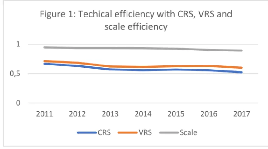
For the whole sample of 485 EU banks during the period 2011-2017, considering constant return to scale (CRS) the overall input oriented technical efficiency measure is TECRS = 0.625. As we said before, if we consider variable returns to scale (VRS), taking into account the variation of the efficiency with respect to the scale of the operation, we get the pure technical efficiency, that is TEVRS = 0.685, revealing that the overall technical inefficiency of the European banks included
12 in our sample is mostly due to inefficient managerial performance and non-efficient combinations of the considered inputs and outputs.
The scale efficiency represents the ability of the management to choose the scale of the production and can be obtained with the ratio TECRS / TEVRS. Here the scale efficiency of the whole sample is 0.912, allowing us to conclude that overall, the bank scale of the considered EU banks over the years 2011-2017 is not very far away from the most productive scale size.
Figure 1 presents the evolution of the technical efficiency with CRS and with VRS as well as the scale efficiency during the considered interval. There is evidence that both TECRS and TEVRS decreased between 2011 and 2013 and that they did not recover during the rest of the interval. The scale efficiency was rather stable, but it slightly decreased during the second part of the considered period.
Annex III presents the average scores of the TECRS, TEVRS and scale efficiency by EU country. The results reported show that despite the country specificities (and the different weight of the banks of each EU country in our sample) the scale efficiency is always higher than the technical and the pure technical efficiency.
4.2. Technical, allocative and cost efficiency
In order to estimate the cost efficiency, we need not only the chosen outputs and inputs but also information regarding the price of the inputs. Still following the intermediation approach, and the
0 0,5 1
2011 2012 2013 2014 2015 2016 2017 Figure 1: Techical efficiency with CRS, VRS and
scale efficiency
13 data available in the Moody’s Analytics BankFocus database, we will consider that the price of the borrowed funds can be represented by the ratio of the interest expense to the deposits and short term funding; the price of the capital and labour is proxied by the ratio of the non-interest expense to total assets. As we want to take into account the relevance of the risk preferences, we include the equity in the inputs and here we will also use the ratio of the equity to total assets. Under these conditions, allocative and cost efficiency can be obtained testing the selection of the inputs, given their prices, that is, the choice of the best combination of inputs to produce the outputs at minimum cost. Following the methodology presented in the previous section, allocative efficiency (AE) will be the ratio of the cost efficiency (CE) to the technical efficiency (TE), and we can consider either constant return to sale (CCR) or variable return to scale (VRS).
Considering CRS, and the whole sample of 485 EU banks over the years 2011-2017, we confirm that the average technical efficiency is 0.625 and we obtain the values of the cost efficiency (CECRS = 0.262) and of the allocative efficiency (AECRS = 0.419). The results with VRS confirm the increase of bank efficiency when we consider that the scale is not constant, now we obtain: TEVRS = 0.685; CEVRS = 0.304 and AECRS = 0.688.
Figures 2 and 3 present the technical, cost and allocative efficiency confirming the similar evolution of the values obtained with CRS and VRS during the interval, as well as the relatively higher values of the efficiency calculated with VRS.
Annex IV reports the DEA country average scores for the technical, allocative and cost efficiency obtained with constant and variable returns to scale.
0 0,5 1
2011 2012 2013 2014 2015 2016 2017
Figure 2: Techical, allocative and cost efficiency (with CRS)
TE AE CE
0 0,5 1
2011 2012 2013 2014 2015 2016 2017
Figure 3: Techical, allocative and cost efficiency (with VRS)
14 4.3. Malmquist indices measuring the technical and productivity changes
The calculation of the Malmquist indices allows us not only to measure the annual productivity changes but also to decompose the changes into the technological changes and the technical efficiency changes.
Technological change measures technological progress (if the values are greater than one) or regress (with values lower than one). The progress may be understood as the banks’ efficient frontier shifting out as a result of the adoption of new technologies by the most efficient banks. The Malmquist indices also report the results of the technical efficiency change (with constant returns to scale) the pure technical efficiency change (with variable returns to scale), the scale efficiency change and the total factor productivity change. Values greater than one always indicate positive changes between one year and the next one.
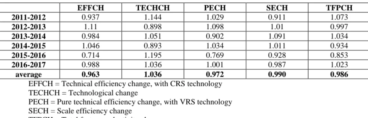
Table 1 – Results obtained for the Malmquist indices
EFFCH TECHCH PECH SECH TFPCH
2011-2012 0.937 1.144 1.029 0.911 1.073 2012-2013 1.11 0.898 1.098 1.01 0.997 2013-2014 0.984 1.051 0.902 1.091 1.034 2014-2015 1.046 0.893 1.034 1.011 0.934 2015-2016 0.714 1.195 0.769 0.928 0.853 2016-2017 0.988 1.036 1.001 0.987 1.023 average 0.963 1.036 0.972 0.990 0.986
EFFCH = Technical efficiency change, with CRS technology TECHCH = Technological change
PECH = Pure technical efficiency change, with VRS technology SECH = Scale efficiency change
TFPCH = Total factor productivity change
Table 1 reports the results obtained for the five Malmquist indices in our sample of EU banks. Overall, the average results reveal that during the considered period the technological changes (TECHCH) were the most dynamic meaning that new and more productive technologies were adopted by the most efficient banks.
Moreover, and confirming the results reported before, there is evidence that, on average, there was no clear progress regarding the technical efficiency changes (ETTCH), the pure technical efficiency changes (PECH), the scale efficiency change (SECH) nor the total factor productivity
15 change (TFPCH). Not surprisingly, the results also reveal that the changes in the technical efficiency change with CRS technology (EFFCF) are clearly in line with the changes in the pure technical efficiency with VRS technology (PECH).
Annex V represents these annual changes of the five Malmquist indices and Annex VI provides the visualisation of the evolution of each of these five indices during the considered period.
4.4. Panel estimates to explain the contributions to the productivity changes ATÉ 30.10.2019 In the second stage of our estimates we will analyse the influence of some bank performance indicators and production conditions to explain the total factor productivity change that we obtained in the previous section.
More precisely, we will use panel data to estimate the linear model represented with equation (7) where the depended variable is the total factor productivity change obtained for each i DMU at time t and considering the following explanatory variables:
Profit before tax to average assets ratio measures the profitability of the bank and is supposed to be in line with the bank’s productivity.
Fixed assets are the bank tangible assets such as property, plant or equipment that can be used to generate income and as collateral to secure long-term debts. Overall, a more productive bank is supposed to have conditions to increase its fixed assets and the increase of the fixed assets may also contribute to the bank’s total factor productivity change.
Net interest margin measures the difference between the interest income generated by the bank and the interest paid out to its lenders relative to the amount of their interest-earning assets. In normal times, the increase of the net interest margins is supposed to be in line with the bank’s productivity.
Impaired loans to equity ratio representing the relation between the doubtful loans and the bank’s equity (that is usually considered as the first cushion for the problems or stress periods). The increase of this ratio is not supposed to benefit the bank’s total factor productivity change.
16 Off-balance sheet items to total assets ratio representing the relevance of the items that are assets or debts of the banks but do not appear in the bank’s balance sheet. The increase of the off-balance sheet items is usually justified with risk transfer, liquidity enhancement and regulation requirements, motives that, overall, would benefit bank performance and therefore contribute to the bank’s productivity growth.
Cost to income ratio measures the overheads or costs of operating the bank, as it is calculated by the division of the operating expenses to the operating income generated by the bank’s activities. The increase of cost to income ratio reveals bank inefficiency and is not supposed to benefit the bank’s total factor productivity change.
Z-score is represented by the sum of the return on assets (ROA) and the equity to total assets ratio (E/TA) divided by the standard deviation of the ROA. Z-score can be considered as an indicator of the risk or probability of banking failure or bankruptcy. A high Z-score indicates low probability of bankruptcy and therefore, the increase of this measure is supposed to benefit the bank’s total factor productivity change.
The use of a panel data approach not only guarantees more observations for the estimations, but also reduces the possibility of multicollinearity among the different variables. The results obtained with the Hausman (1978) test1 recommend the use of panel random-effects estimates. In a panel random-effects model we suppose that the individual specific effect of each DMU (here, each EU bank included in our sample) is a random variable that is uncorrelated with the explanatory variables.
17
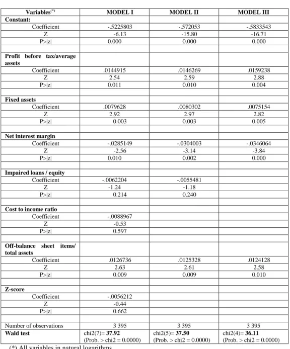
Table 2 – Results obtained with panel random-effects estimates Variables(*) MODEL I MODEL II MODEL III
Constant:
Coefficient -.5225803 -.572053 -.5833543
Z -6.13 -15.80 -16.71
P>|z| 0.000 0.000 0.000
Profit before tax/average assets Coefficient .0144915 .0146269 .0159238 Z 2.54 2.59 2.88 P>|z| 0.011 0.010 0.004 Fixed assets Coefficient .0079628 .0080302 .0075154 Z 2.92 2.97 2.82 P>|z| 0.003 0.003 0.005
Net interest margin
Coefficient -.0285149 -.0304003 -.0346064
Z -2.56 -3.14 -3.84
P>|z| 0.010 0.002 0.000
Impaired loans / equity
Coefficient -.0062204 -.0055481
Z -1.24 -1.18
P>|z| 0.214 0.240
Cost to income ratio
Coefficient -.0088967
Z -0.53
P>|z| 0.597
Off-balance sheet items/ total assets Coefficient .0126736 .0125328 .0124128 Z 2.63 2.61 2.58 P>|z| 0.009 0.009 0.010 Z-score Coefficient -.0056212 Z -0.44 P>|z| 0.662 Number of observations 3 395 3 395 3 395
Wald test chi2(7)= 37.92 (Prob. > chi2 = 0.0000)
chi2(5)= 37.50 (Prob. > chi2 = 0.0000)
chi2(4)= 36.11 (Prob. > chi2 = 0.0000) (*) All variables in natural logarithms.
Table 2 reports the results obtained using panel random-effects estimates. For the three considered models the results of the Wald test allow us to conclude that the estimates are in general robust.
In all situations and as expected, there is clear evidence that profit before tax to average assets ratio and the fixed assets positively contribute to the banks’ total factor productivity change. On the other side, and also as expected (although not with the same statistical significance) the
18 impaired loans to equity and the cost to income ratios have a negative influence in banks’ productivity.
A relative surprise may be the negative influence of the net interest margins in the banks’ productivity. But it is an understandable result if we take into account the historical low level of the interest rates (decreasing also the margins) during the considered period.
The clear positive influence that the off-balance sheet items to total assets ratio has in the banks’ total factor productivity change confirm the relevance of the off-balance sheet items in the banks’ activities, contributing to risk transfer, liquidity enhancement and overcoming the challenges of the regulation requirements.
The results obtained for the Z-score point to its negative influence (although not statistically very strong) in the banks’ productivity, allowing us to conclude that, at least in our sample and using the adopted measure of Z-score, there is no convincing evidence that the probability of bankruptcy is in line with the banks’ total factor productivity change.
5. Concluding Remarks
This paper uses Data Envelopment Analysis (DEA) techniques to measure and analyse the European bank efficiency between 2011 and 2017, considering a sample of 485 banks from all current EU member-states. Following the intermediation approach banks are assumed to produce three outputs: loans, other earning assets, and non-earning assets using three inputs: interest expenses, non-interest expenses, and equity. All data are sourced from the Moody’s Analytics BankFocus database.
We adopt a two-stage approach. In the first stage we obtain different measures of DEA bank efficiency. We begin with the estimation of technical efficiency, pure technical efficiency and scale efficiency. The results obtained reveal the existence of bank inefficiency, and that this inefficiency is mostly due to inefficient managerial performance and non-effective combinations of the considered bank inputs and outputs. In what regards to the scale efficiency there is evidence
19 of overall ability of the management to choose the scale of production. The existence of bank inefficiency is confirmed when we measure the allocative and the cost efficiency, and the bank efficiencies are particularly low when we consider constant returns to scale.
The calculation of the Malmquist indices allows us to measure not only the annual productivity changes but also to decompose the changes into the technological changes and the technical efficiency changes. Overall, the average results reveal that during the considered period the technological changes were the most dynamic meaning that new and more productive technologies were adopted by the most efficient banks. In addition, and confirming the results obtained before, there is evidence that, on average, there was no clear progress regarding the technical efficiency changes, the pure technical efficiency changes, the scale efficiency change nor the total factor productivity change.
In the second stage we use panel random effects estimates to analyse the influence of some bank performance indicators and production conditions to explain the total factor productivity change that we obtained with the Malmquist indices. The results obtained allow us to conclude that, as expected, profit before tax to average assets ratio and the fixed assets contribute positively to the banks’ total factor productivity change, while the impaired loans to equity and the cost to income ratios have a negative influence in banks’ productivity.
There is also clear evidence of the negative influence of the net interest margins in the banks’ productivity, and this is an understandable result considering the historical low level of the interest rates (decreasing also the banks’ margins) in recent years.
The clear positive influence that the off-balance sheet items to total assets ratio has in the banks’ total factor productivity change confirm the relevance of the off-balance sheet items in the banks’ activities, contributing to risk transfer, liquidity enhancement and overcoming the challenges of the regulation requirements, namely those related to the severe crisis that the EU banking institutions had to overcome during the considered period.
Overall, our results confirm the existence of bank technical inefficiencies, mostly due to bad choices in the combinations of the banks’ inputs and outputs as well as to inefficient management. On the other side, our estimations confirm good choices in terms of the scale of the production
20 and appropriate technical efficiency changes at least in the considered sample of EU banks and in the aftermath of the crises that these banks had to overcome during the last decade.
Further research in this field is still needed, namely analysing the determinants of bank efficiency, considering other variables as bank outputs and/or inputs and other samples of EU and non-EU banks.
References
Aiello, F., and Bonanno, G. (2013) Profit and cost efficiency in the Italian banking industry
(2006-2011), MPRA Paper no. 48940.
Aigner, D.J., Lovell C.A.K. and Schmidt, P. (1977) “Formulation and estimation of stochastic frontier production function models”, Journal of Econometrics, 6, pp. 21-37.
Ali, A.I. and Lerme, C.S. (1997) “Comparative advantage and disadvantage in DEA”, Annals of
Operations Research, 73, pp. 215–232.
Ali, A.I. and Seiford, L.M. (1993) “The Mathematical Programming Approach to Efficiency Analysis” in Fried, H.O., Lovell, C.A.K. and Schmidt, S.S. (Eds), The Measurement of Productive
Efficiency, New York, Oxford University Press, pp. 120-159.
Almanza, C. and Rodríguez, J. J. M. (2018) “Profit efficiency of banks in Colombia with undesirable output: a directional distance function approach”, Economics: the Open-Access, Open-Assessment e-Journal, journal article no. 2018-30.
Altunbas, Y., Carbo, S., Gardener, E. P. M. and Molyneux, P. (2007) “Examining the Relationships between Capital, Risk and Efficiency in European Banking”, European Financial Management, 13, pp. 49–70.
Apergis, N. and Polemis, M.L. (2016) “Competition and efficiency in the MENA banking region: a non-structural DEA approach,”, Applied Economics, 48, pp. 5276-5291.
Asmild, M. and Zhu, M. (2016) “Controlling for the use of extreme weights in bank efficiency assessments during the financial crisis”, European Journal of Operational Research, 251, pp. 999-1015.
Banna, H., Shah, S.K.B., Noman, A. H., Ahmad, R. and Masud, M. M. (2019) "Determinants of Sino-ASEAN Banking Efficiency: How Do Countries Differ?", Economies, MDPI, Open Access Journal, 7, pp. 1-23.
Banya, R. and Biekpe, N. (2018) "Banking efficiency and its determinants in selected frontier african markets", Economic Change and Restructuring, 51, pp. 69-95.
Battese, G. E. and Coelli, T. (1988) “Prediction of firm-level technical efficiencies with a generalized frontier production function and panel data”, Journal of Econometrics, 38, pp. 387-399.
21 Battese, G. E. and Coelli, T. (1995) “A Model for Technical Inefficiency Effects in a Stochastic Frontier Production Function for Panel data”, Empirical Economics, 20, pp. 325-332.
Berg, S. (2010) Water Utility Benchmarking: Measurement, Methodology, and Performance
Incentives, London and New York, International Water Association.
Candemir, M., Ozcan, M., Gunes, M. and Delikas, E. (2011) “Technical Efficiency and Total Factor Productivity in the Hazelnut Agricultural Sales Cooperatives Unions in Turkey”,
Mathematical and Computational Applications, 16, pp. 66-76.
Casu, B. and Molyneux, P. (2003) “A comparative study of efficiency in European banking”,
Applied Economics, 35, pp. 1865-1876.
Charnes A., Cooper W.W. and Rhodes, E. (1978) “Measuring the Efficiency of Decision-Making Units”, European Journal of Operational Research, 2, pp. 429 - 444.
Charnes, A., Cooper W.W., Lewin, A.Y. and Seiford, L.M. (1994) Data Envelopment Analysis:
Theory, Methodology and Application, Boston, Kluwer Academic Publishers.
Chen, Z., Matousek, R. and Wanke, P. (2018) "Chinese bank efficiency during the global financial crisis: A combined approach using satisficing DEA and Support Vector Machines", The North
American Journal of Economics and Finance, 43, pp. 71-86.
Chen, T.Y, Chen, C.B. and Peng, S.Y. (2008) “Firm operation performance analysis using data envelopment analysis and balanced scorecard: A case study of a credit cooperative bank”,
International Journal of Productivity and Performance Management, 57, pp. 523-539.
Chortareas, G. E., Girardone, C. and Ventouri, A. (2013) "Financial freedom and bank efficiency: Evidence from the European Union," Journal of Banking & Finance, 37, pp 1223-1231.
Coelli, T. (1996) “A Guide to DEAP Version 2.1: A Data Envelopment Analysis (Computer) Program, CEPA Working Paper 96/08.
Cook, W.D., Tone, K., and Zhu, J. (2014) “Data envelopment analysis: Prior to choosing a model”, OMEGA, 44, pp. 1-4.
Cooper, W.W., Seiford, L.M. and Tone, K. (2006) Data Envelopment Analysis: A Comprehensive
Text with Models, Applications, References and DEA-Solver Software, 2nd Ed., New York, Springer.
Diallo, B. (2018) "Bank efficiency and industry growth during financial crises", Economic Modelling, 68, pp. 11-22.
Degl'Innocenti, M., Kourtzidis, S. A.,Sevic, Z. and Tzeremes, N. G. (2017) "Investigating bank efficiency in transition economies: A window-based weight assurance region approach", Economic Modelling, 67, pp 23-33.
Drake, L. (2001) “Efficiency and productivity change in UK banking”, Applied Financial
Economics, 11, pp. 557–571.
Farrell, M.J. (1957) “The Measurement of Productive Efficiency” Journal of the Royal Statistical
Society, 120, pp. 253-290.
Favero, C.A. and Papi, L. (1995) “Technical efficiency and scale efficiency in the Italian banking sector: a non-parametric approach”, Applied Economics, 27, pp. 385-395.
Fujii, H., Managi, S., Matousek, R. and Rughoo, A. (2018) “Bank efficiency, productivity, and convergence in EU countries: a weighted Russell directional distance model”, The European
Journal of Finance, 24, pp. 135-156.
Fukuyama, H. and Matousek, R. (2018) "Nerlovian revenue inefficiency in a bank production context: Evidence from Shinkin banks," European Journal of Operational Research, 271, pp. 317-330.
22 Grigorian, D.A. and Manole, V. (2016) Sovereign Risk and Deposit Dynamics: Evidence from
Europe, IMF Working Paper, No. 16/145.
Hausman, J.A. (1978) “Specification tests in econometrics”, Econometrica, 46, (6), pp. 1251–71. Johnes, J. (2006) “Data envelopment analysis and its application to the measurement of efficiency in higher education”, Economics of Education Review, 25, pp. 273-288.
Kocisova, K. (2017) “Measurement of Revenue Efficiency in European Union Countries: A Comparison of Different Approaches”, International Journal of Applied Business and Economic
Research, 15, pp. 31-42.
Kuc, M. (2018) Cost Efficiency of European Cooperative Banks, Institute of Economic Studies (IES) Working paper 21/2018.
Kumar, M., Charles, V. and Mishra, C. S. (2016) "Evaluating the performance of Indian banking sector using DEA during post-reform and global financial crisis", Journal of Business Economics
and Management, 17, pp. 156-172.
Kumar, S. and Gulati, R. (2008) “An Examination of Technical, Pure Technical, and Scale Efficiencies in Indian Public Sector Banks using Data Envelopment Analysis”, Eurasian Journal
of Business and Economics, 1, pp. 33-69.
Lovell, C.A.K. (1993) “The Mathematical Programming Approach to Efficiency Analysis” in Fried, H.O., Lovell, C.A.K. and Schmidt, S.S, (Eds), The Measurement of Productive Efficiency, New York, Oxford University Press, pp. 3-67.
Lozano-Vivas, A., Kumbhakar, S.C., Fethi, M.D. and Shaban, M. (2011) “Consolidation in the European banking industry: How effective is it?”, Journal of Productivity Analysis, 36, pp. 247-261.
Novickytė. L. and Droždz, J. (2018) "Measuring the Efficiency in the Lithuanian Banking Sector: The DEA Application," International Journal of Financial Studies, MDPI, Open Access Journal,
6, pp. 1-15.
Okuda, H. and Aiba, D. (2016) "Determinants of Operational Efficiency and Total Factor Productivity Change of Major Cambodian Financial Institutions: A Data Envelopment Analysis During 2006–13", Emerging Markets Finance and Trade, 52, pp. 1455-1471.
Oliveira, J. (2017) Inefficiency distribution of the European Banking System, Banco de Portugal, Working Paper No. 12.
Ouenniche, J. and Carrales, S. (2018) “Assessing efficiency profiles of UK commercial banks: a DEA analysis with regression-based feedback”, Annals of Operations Research, 266, pp. 551-587.
Partovi, E. and & Matousek, R. (2019) "Bank efficiency and non-performing loans: Evidence from Turkey," Research in International Business and Finance, 48, pp. 287-309.
San-Jose,L. Retolaza, J. L. and and Lamarque, E. (2018) “The Social Efficiency for Sustainability: European Cooperative Banking Analysis”, Sustainability, 10, pp. 1-21.
Shah, A.A., Wu, D. and Korotkov, V. (2019) "Are Sustainable Banks Efficient and Productive? A Data Envelopment Analysis and the Malmquist Productivity Index Analysis," Sustainability, MDPI, Open Access Journal, 11, pp. 1-19.
Sharif, O., Hasan, Z., Fah, C. Y. and & Sirdari, M. Z. (2019) "Efficiency analysis by combination of frontier methods: Evidence from unreplicated linear functional relationship model," Business
and Economic Horizons (BEH), Prague Development Center (PRADEC), 15, pp. 107-125.
Sherman, H.D. and Zhu, J. (2006) Service Productivity Management: Improving Service Performance using Data Envelopment Analysis (DEA), New York, Springer.
23 Sherman, H.D. and Zhu, J. (2013) “Analysing performance in service organizations”, Sloan
Management Review, 54, pp. 37-42.
Tanna, S., Pasiouras, F. and Nnadi, M. (2011) “The effect of board size and composition on the efficiency of UK banks”, International Journal of the Economics of Business, 18, pp. 441–462. Tuskan, B. and Stojanovic, A. (2016) “Measurement of cost efficiency in the European banking industry”, Croatian Operational Research Review, 7, pp. 47-66.
Vozková, K. and Kuc, M. (2017) “Cost Efficiency of European Cooperative Banks”,
International Journal of Economics and Management Engineering, 11, pp. 2705-2708.
Wanke, P., Azad, Md A. K., Emrouznejad, A. and Antunes, J. (2019) "A dynamic network DEA model for accounting and financial indicators: A case of efficiency in MENA banking",
International Review of Economics & Finance, 61, pp. 52-68.
Wanke, P., Barros, C.P., Azad, Md A.K. and Constantino, D. (2016) "The Development of the Mozambican Banking Sector and Strategic Fit of Mergers and Acquisitions: A Two-Stage DEA Approach", African Development Review, 28, pp. 444-461.
Webb, R. (2003) “Levels of efficiency in UK retail banks: A DEA window analysis”,
International Journal of the Economics of Business, 10, pp. 305–322.
Wooldridge, J. M., 2010. Econometric Analysis of Cross Section and Panel Data. the MIT Press. Yu, Y., Huang, J. and Shao, Y. (2019) "The Sustainability Performance of Chinese Banks: A New Network Data Envelopment Analysis Approach and Panel Regression," Sustainability, MDPI, Open Access Journal, 11, pp. 1-25.
24 ANNEX I – A selection of recent studies on DEA bank efficiency
Autor(s) and year Country or region Period of analysis Main findings Apergis and Polemis, (2016) Middle East and North Africa (MENA) countries
1997-2011 The level of bank efficiency was estimated by
using the nonparametric methodology of the DEA. From the empirical findings, the paper concluded that the average cost efficiency in the MENA banking region was relatively high (77.6%), denoting that MENA banks need to improve only by 22.4, to reach the cost efficiency frontier. It is important to note that there was not any significant variation in the level of cost efficiency across MENA countries. Banna et al, (2019) Sino-ASEAN region
2000-2013 The results obtained suggest that during the pre-crisis period, banks belonging to China and Indonesia were more likely to be efficient due to the geographical location effect. Overall, the results suggest that Chinese banks outperform banks from the ASEAN countries in terms of efficiency. Banya and Biekpe, (2018) 10 frontier African countries
2008-2012 The results of the analysis show that, to a greater extent, banks in the countries studied have efficient banking sectors. The results of truncated regression indicate that bank size is negatively related to banking sector efficiency while the degree of risk is positively related to bank efficiency.
Chen et al, (2018)
China 2008-2011 The findings undoubtedly confirm that the performance of the Chinese banks is rather weak. Inefficiency across all the spectrum of banks are rather alarming and NPLs as well as a proper bank corporate governance require to be carefully addressed.
Diallo, (2018) 38 countries from different Continents
2009 The main result shows that bank efficiency relaxed credit constraints and increased the growth rate for financially dependent industries during the crisis. This finding shows the great but overlooked importance of bank efficiency in mitigating the negative effects of financial crises on growth.
Fukuyama and Matousek, (2018)
Japan 2007-2015 The paper discusses inefficiency scores by using slack-based allocative and technical inefficiency. The decomposition of Nerlovian revenue inefficiency into slack-based technical inefficiency (SBTI) and slack-based allocative inefficiency (SBAI) reveals that the main source of bank inefficiency comes from SBTI. Kumar et al,
(2016)
India 1995-2010 The main contribution of the paper is to empirically provide the evidences to resolve the debate if the global financial crisis had any impact on the performance of banking sector in India. The empirical results reveal that substantial gains could be obtained from altering scale of the public sector banks via either internal growth or consolidation in the sector.
Novickytė and Droždz, (2018)
Lithuania 2012-2016 The Lithuanian bank’s efficiency analysis based on the VRS assumption shows that better results are demonstrated by the local banks. The technical efficiency analysis based on the CRS assumption shows other results: the banks owned by the Nordic parent group and the branches have higher pure efficiency than local banks and have success at working at the right scale.
Okuda and Aiba, (2016)
Cambodia 2006-2013 The empirical results reveal that the size and ownership structure of financial institutions are significantly correlated with the efficiency and TFP growth of banks. The efficiency of domestic institutions is found to be better than that of their foreign counterpart, and there is no significant difference in TFP growth between domestic and foreign institutions.
Ouenniche and Carrales, (2018)
UK 1987-2015 Empirical results suggest that, on average, the commercial banks operating in the UK—whether domestic or foreign—are yet to achieve acceptable levels of overall technical efficiency, pure technical efficiency, and scale efficiency. Furthermore, in general, a linear regression-based feedback mechanism proves effective at improving discrimination in DEA analyses unless the initial choice of inputs and outputs is well informed.
Partovi and Matousek, (2019)
Turkey 2002-2017 Non-Performing Loans exert a negative impact in terms of technical efficiency, confirming the “bad management” hypothesis in the banking sector. The level of efficiency of Turkish banks differs, depending on the ownership structure.
25 Shah et al, (2019) 14 counties from Asia, Europe, North America and South America
2010-2018 Sustainable banks (SBs) are more efficient and have higher productivity than non-sustainable banks (NSBs). SBs and NSBs in different regions differ in efficiency.
Sharif et al, (2019)
Malaysia 2007-2016 The paper provides a combination of DEA and SFA efficiency scores, underlying the differences in the scores obtained. It identifies the most efficient and the less efficient financial firms. Wanke et al,
(2016)
Mozambique 2003-2013 The results obtained reveal that ownership (public or foreign) impacts virtual efficiency levels. The findings also show that care must be exercised with M&A because the resultant banking organization could be oversized when foreign ownership is predominant, especially when public ownership is low. Given the relative sizes of the markets in terms of productive resources, M&A involving Mozambican banks can easily lead to decreasing returns to scale. Wanke et al, (2019) Middle East and North Africa (MENA) countries
2006-2014 The results reinforce the existence of regulatory marks and culture barriers that may explain why similar countries in size and geographical location may be performing differently in the banking industry.
Yu et al, (2019)
China 2010-2014 The efficiency of the considered banks shows heterogeneity and the efficiency of most foreign banks has much room for improvement. Liquidity and scale effects exert positive impacts on bank efficiency.
Annex II – Number of banks by EU member-state
EU country Number of banks % of the total banks
Austria 20 4.12 Belgium 7 1.44 Bulgaria 5 1.03 Croatia 7 1.44 Cyprus 3 0.62 Czech Rep. 8 1.65 Denmark 31 6.39 Estonia 2 0.41 Finland 5 1.03 France 43 8.87 Germany 103 21.24 Greece 6 1.24 Hungary 7 1.44 Ireland 4 0.82 Italy 105 21.65 Latvia 1 0.21 Lithuania 4 0.82 Luxembourg 9 1.86 Malta 3 0.62 Netherlands 16 3.30 Poland 14 2.89 Portugal 6 1.24 Romania 4 0.82 Slovakia 7 1.44 Slovenia 6 1.24 Spain 13 2.68 Sweden 7 1.44 UK 39 8.04
26
Annex III – DEA country average technical efficiency scores EU country Technical efficiency
with CRS Technical efficiency with VRS Scale efficiency Austria 0.570 0.725 0.786 Belgium 0.426 0.498 0.855 Bulgaria 0.611 0.736 0.830 Croatia 0.528 0.590 0.895 Cyprus 0.450 0.478 0.941 Czech Rep. 0.537 0.613 0.876 Denmark 0.614 0.642 0.956 Estonia 0.465 0.465 1.000 Finland 0.681 0.730 0.933 France 0.838 0.845 0.992 Germany 0.575 0.649 0.886 Greece 0.473 0.477 0.992 Hungary 0.509 0.515 0.988 Ireland 0.624 0.634 0.984 Italy 0.599 0.696 0.861 Latvia 0.800 1.000 0.800 Lithuania 0.930 0.997 0.933 Luxembourg 0.833 0.944 0.882 Malta 0.906 0.944 0.960 Netherlands 0.84 0.867 0.969 Poland 0.713 0.728 0.979 Portugal 0.724 0.726 0.997 Romania 0.871 0.873 0.998 Slovakia 0.488 0.504 0.968 Slovenia 0.664 0.690 0.962 Spain 0.485 0.500 0.970 Sweden 0.492 0.583 0.844 UK 0.584 0.615 0.950
Source: Author’s calculations
Annex IV – DEA country average technical, allocative and cost efficiency scores (with CRS and VRS)
EU country TECRS AECRS CECRS TEVRS AEVRS CEVRS Austria 0.570 0.411 0.234 0.725 0.323 0.234 Belgium 0.426 0.453 0.193 0.498 0.392 0.195 Bulgaria 0.611 0.381 0.233 0.736 0.318 0.234 Croatia 0.528 0.650 0.343 0.590 0.585 0.345 Cyprus 0.450 0.638 0.287 0.478 0.600 0.287 Czech Rep. 0.537 0.337 0.181 0.613 0.299 0.183 Denmark 0.614 0.300 0.184 0.642 0.291 0.187 Estonia 0.465 0.357 0.166 0.465 0.368 0.171 Finland 0.681 0.410 0.279 0.730 0.385 0.281 France 0.838 0.690 0.578 0.845 0.710 0.600 Germany 0.575 0.449 0.258 0.649 0.462 0.300 Greece 0.473 0.347 0.164 0.477 0.356 0.170 Hungary 0.509 0.263 0.134 0.515 0.283 0.146 Ireland 0.624 0.399 0.249 0.634 0.438 0.278 Italy 0.599 0.379 0.227 0.696 0.444 0.309 Latvia 0.800 0.943 0.754 1.000 1.000 1.000 Lithuania 0.930 0.749 0.697 0.997 0.967 0.964 Luxembourg 0.833 0.630 0.525 0.944 0.654 0.617 Malta 0.906 0.572 0.518 0.944 0.738 0.697 Netherlands 0.840 0.383 0.322 0.867 0.370 0.321 Poland 0.713 0.139 0.099 0.728 0.147 0.107 Portugal 0.724 0.594 0.430 0.726 0.687 0.499 Romania 0.871 0.834 0.726 0.873 0.869 0.759 Slovakia 0.488 0.096 0.047 0.504 0.123 0.062 Slovenia 0.664 0.063 0.042 0.690 0.068 0.047 Spain 0.485 0.293 0.142 0.500 0.324 0.162 Sweden 0.492 0.201 0.099 0.583 0.196 0.114 UK 0.584 0.245 0.143 0.615 0.278 0.171
27
Annex V – Annual results of all the Malmquist indices
EFFCH = Technical efficiency change, with CRS technology TECHCH = Technological change
PECH = Pure technical efficiency change, with VRS technology SECH = Scale efficiency change
TFPCH = Total factor productivity change
0 0,2 0,4 0,6 0,8 1 1,2 1,4 2011-2012 2012-2013 2013-2014 2014-2015 2015-2016 2016-2017 EFFCH TECHCH PECH SECH TFPCH
28
VI – Annual results of each of the five Malmquist indices
0 0,5 1 1,5
2011-2012 2012-2013 2013-2014 2014-2015 2015-2016 2016-2017 EFFCH = Technical efficiency change (with CRS technology)
0 0,5 1 1,5
2011-2012 2012-2013 2013-2014 2014-2015 2015-2016 2016-2017 TECHCH = Technological change
0 0,5 1 1,5
2011-2012 2012-2013 2013-2014 2014-2015 2015-2016 2016-2017 PECH = Pure technical efficiency change (with VRS technology)
0,8 0,9 1 1,1 1,2 2011-2012 2012-2013 2013-2014 2014-2015 2015-2016 2016-2017 SECH = Scale efficiency change
0 0,5 1 1,5
2011-2012 2012-2013 2013-2014 2014-2015 2015-2016 2016-2017 TFPCH = Total factor productivity change