Theoretical perspectives on the
dynamics of communities with
intraguild predation
Gabriel Andreguetto Maciel
dynamics of communities with
intraguild predation
Thesis
submitted to the Institute for Theoretical Physics
São Paulo State University, Brazil
as a partial fulfillment of the requirements for the degree of
Master of Science
February 2011
Gabriel Andreguetto Maciel
Examination Committee
Roberto André Kraenkel IFT-UNESP, São Paulo
André M. de Roos University of Amsterdam
Marcus A. M. de Aguiar IFGW-UNICAMP, Campinas
Claudia Pio Ferreira
IBB-UNESP, Botucatu (substitute)
Hilda Cerdeira
IFT-UNESP, São Paulo (substitute)
and Ana Carolina
Abstract
Intraguild predation is a widespread interaction between species and can strongly influence communities composition. It occurs when two consumers which share a common resource, and hence compete, also engage into predation. The con-sumer which can prey on its competitor is often referred to as the intraguild predator while the other is called intraguild prey. In this work we investigate some theoretical aspects about these interactions. First we analyse an experi-ment with predatory mites which was carried to test patterns of exclusion along a productivity gradient, predicted by theory. Although this experiment was care-fully designed to test the theoretical assertions, their results do not agree with theory. Through a very simple model for intraguild predation which serves as a representation of that system, we show that: if the short-term dynamics is taken into account rather than only equilibrium states, in which the usual theory is based, and we consider that populations that attain levels very close to zero are extinct, experimental results meet theory. Then we study questions concerning the influence of different life stages of individuals on the dynamics of intraguild predation. We introduce a model with stage structure in both consumers and consider predation occurring only from adults of the intraguild predator on juve-niles of the intraguild prey. This stage dependent interaction was believed to have great effects on the dynamics, once predation pressure on the intraguild prey is reduced, and has been proposed as one feature that could promote coexistence. We check the outcomes of the system along a productivity gradient and show that stage structure do not induce great qualitative changes on the dynamics and the more likely resulting dynamics continues being the extinction of one of the consumers. Predation between consumers can also be reciprocal and this phe-nomenon is ubiquitous in many systems. In the last part of this work we study a model for reciprocal intraguild predation in a stage structured system. Increasing the attack rates of that consumer which was initially the intraguild prey on the intraguild predator we find that a reciprocal intraguild predation system has a great potential for alternative states in which each consumer can persist isolated with resource, initial conditions determining what consumer will persist.
Predação intraguilda é um tipo de interação muito comum entre as espécies e pode influenciar fortemente na composição das comunidades ecológicas. Ela ocorre quando dois consumidores que compartilham de um mesmo recurso, e portanto competem, também apresentam comportamento predatório entre si. O consumi-dor que preda o seu competiconsumi-dor é frequentemente chamado de predaconsumi-dor intra-guilda, enquanto aquele que é predado é conhecido como presa intraguilda. Nesse trabalho nós investigamos alguns aspectos teóricos sobre esse tipo de interação. Primeiramente analisamos um experimento com ácaros predadores que foi reali-zado para testas as predições da teoria sobre padrões de exclusão em um gradiente de produtividade. Embora esse experimento foi cuidadosamente projetado para testar afirmações da teoria, seus resultados não concordam com ela. Utilizando um modelo bem simples para predação intraguilda que serve como uma repre-sentação daquele sistema, nós mostramos que: se levarmos em conta a dinâmica durante os transientes, e não apenas os resultados no equilíbrio, em que a teoria usual se baseia, e considerarmos que quando uma população atinge níveis muito baixos corresponde a uma extinção na realidade, os resultados experimentais con-cordam com a teoria. Em seguida nós estudamos questões que dizem respeito a influência dos diferentes estágios de vida dos indivíduos para a dinâmica da pre-dação intraguilda. Nós introduzimos um modelo com estrutura de estágio em ambos os consumidores e consideramos a predação ocorrendo apenas dos adultos do predador intraguilda sobre os juvenis da presa intraguilda. Tem-se acreditado que essa interação dependente de estágio pode ter grandes efeitos sobre a dinâ-mica, uma vez que a pressão predatória sobre a presa intraguilda é reduzida nesse caso, e foi proposta como uma característica que poderia promover coexistência. Obtivemos a dinâmica do sistema ao longo de um gradiente de produtividade e mostramos que a estrutura de estágios não induz grandes mudanças qualitativas na sua dinâmica, continuando a extinção de um dos consumidores o resultado mais provável do sistema. A predação entre os consumidores também pode ser recíproca. Esse fenômeno é bastante frequente em muitos sistemas. Na última parte desse trabalho nós estudamos um modelo para predação intraguilda recí-proca em um sistema com estrutura de estágios. Aumentando as taxas de ataque
daquele consumidor que inicialmente era a presa intraguilda sobre o predador intraguilda nós mostramos que um sistema com predação intraguilda recíproca tem um grande potencial para apresentar bistabilidade, onde cada consumidor pode persistir isolado com o recurso, as condições iniciais determinando qual dos consumidores persistirá.
Abstract vii Abstract in Portuguese ix
Acknowledgments xiii
1 Introduction 1
1.1 The intraguild predation module . . . 3
1.2 Models for population biology . . . 4
1.2.1 Models for a single species . . . 5
1.2.2 Models for interacting populations . . . 6
1.3 Theoretical perspectives on IGP . . . 7
2 Theory of intraguild predation 9 2.1 General model for simple IGP . . . 9
2.2 Necessary condition for coexistence . . . 10
2.3 Logistic resource growth . . . 12
2.3.1 Stationary states . . . 12
2.3.2 Stability of the stationary states . . . 13
3 Tests of the theory 17 3.1 Experiment with mites . . . 17
4 Transient dynamics in the simple IGP module 23 4.1 Transient dynamics and patterns of exclusion of mites . . . 24
5 IGP and stage structure 29 5.1 Stage structure in both consumers . . . 30
5.1.1 The model . . . 30
5.1.2 Both consumers with stages x stage structure in only one of consumers . . . 36
5.1.3 Lifetime fractions . . . 37
6 Reciprocal IGP in stage structured systems 41
6.1 Equations representing the system . . . 42 6.1.1 Equilibrium points . . . 42 6.2 States dependence on environmental productivity . . . 44
7 Conclusions 49
A Parameters estimation 53
A.1 Resource growth . . . 53 A.2 Resource consumption abilities . . . 54 A.3 β and α . . . 55
Thanks to CNPq and CAPES for financial support.
To Arne Janssen and Sara Magalhães which enormously helped improve this the-sis.
I thank to José Danilo, for helping me in the task of moving to São Paulo and living in this city.
The work described here was a joint effort with my supervisor, Roberto Kraenkel, and I am deeply grateful for the opportunity to have worked with him.
During preparation of this thesis I was very fortunate to have nice colleagues in our research group. Thanks to Anderson, Franciane, Juliana, Natarajan and Renato for every suggestion on my work and for moments of leisure.
To my sisters, Letícia and Juliana, for our friendship and for I can always count on them.
Thanks to Ana Carolina for her love and for always encouraging me on my dreams.
Finally, thanks to my parents, Ariovaldo and Ana Verginia, that with great love support every step of my life.
São Paulo Gabriel Andreguetto Maciel
February, 2011.
1
Introduction
Pairwise interactions such as competition and predation are very simple ecologi-cal relations. Although it is known that frequently species are immersed in very complex food webs, composed of several interacting species which compose an ecological community, the study of these simple interactions is of great impor-tance. To cite two important examples, the description of mechanisms leading to oscillations in predator-prey systems and the principle of competition exclu-sion led to great advances in theoretical ecology [Murray, 2002]. It is upon these pairwise relations that a great part of population biology theory is built.
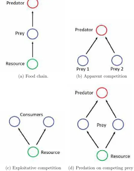
Between the bewildering complexity and richness of natural communities, and the simplicity of single population dynamics or pairwise interactions, a useful ap-proach in the study of population dynamics is to consider community modules. Community modules are systems consisting of a small number of species linked by a specified interaction structure. Some familiar examples of modules are: food chains, apparent competition, exploitative competition and predation on compet-ing prey (also known as keystone predation). These interactions are schematized in figures 1.1a-d. In some cases, systems under study are very similar to a partic-ular module, for it can be created in laboratory or it can be a system composed of few species interacting strongly. Furthermore, its expected that the study of community modules, at least in a qualitative way, reveals the behaviour of more complex communities [Holt, 1995].
(a) Food chain. (b) Apparent competition
(c) Exploitative competition (d) Predation on competing prey
1.1. The intraguild predation module 3
1.1
The intraguild predation module
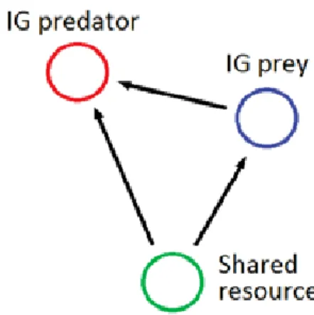
One module that has been accepted as being of great interest is that of intraguild predation (figure 1.2). This system, in its simplest form, is composed of two species which share a common vital resource, hence they compete, and addition-ally they engage in predation [Polis and Holt, 1992; Polis et al., 1989].
Figure 1.2: The intraguild predation module.
These consumer species are said to be members of a “guild”, defined according to Root [1967] as “ a group of species that exploit the same class of environmental resources in a similar way”. Intraguild predation (IGP) combines elements of both competition and predation and influences significantly distribution, abundance and evolution of many species [Polis and Holt, 1992]. Because consumer species can prey on more than one trophic level, IGP is also a subset of omnivory [Pimm and Lawton, 1978].
Only recently IGP has received greater attention by both empiric and the-oretical studies, possibly because thethe-oretical results point out that IGP has a destabilizing effect on communities (that is, coexistence of consumers is only pos-sible in very restricted conditions, see chapter 2), and, in this way, we would not expect so many examples in nature [Mylius et al., 2001]. However, it has become clear now that this module is ubiquitous in nature, and it is present in both freshwater, marine and terrestrial food webs [Polis and Holt, 1992; Polis et al., 1989].
In the simplest IGP module there is a top predator, frequently called intraguild predator (IG predator), which preys on its competitor (the intraguild prey (IG prey)). Competition is mediated by the consumption of a shared resource (see figure 1.2). There are many variations of this IGP composition.
frequently face great changes in their abilities for feeding, reproducing, avoiding predation (in the case of prey species), among other ecological relevant processes. In some cases adults of the prey can grow too large, resulting in that they become invulnerable to predation, creating a “prey size refugium” [Chase, 1999]. Many predation interactions in IGP are restricted to particular ages or stages [Polis et al., 1989]. Prey size refugia attenuate predation strength between IG prey and IG predator, and has been proposed as a potential mechanism promoting species persistence in IGP [Mylius et al., 2001; Polis and Holt, 1997]. We will address the consequences of including stage structure in models for IGP in chapter 5.
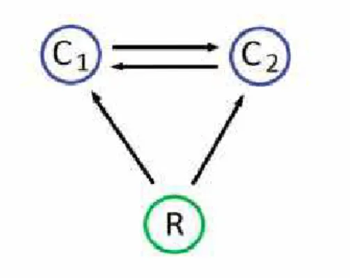
When both consumers can prey on each other we have a module called recip-rocal IGP (also known as symmetric IGP or crossed IGP). These interactions are very common in nature [Polis et al., 1989], but only few works have focused on its consequences for the community structure [HilleRisLambers and Dieckmann, 2003; van der Hammen et al., 2010]. Figure 1.3 shows an scheme of symmetric IGP. Both competitors, C1 and C2, can prey on each other, and then the
nomen-clature IG predator and IG prey is nonsense here 1
. This IGP variant is also commonly found between species which suffer ontogenetic diet shifts.
Figure 1.3: Symmetric IGP. Competitors, C1and C2, engage in mutual predation.
Given the omnipresence of these features in IGP, its of great interest the study of their implications for the evolution of IGP. Using models for populations dynamics, we approach these questions in chapters 5 and 6.
1.2
Models for population biology
A main question that comes naturally in population biology is to know how systems change with time. Mathematical models are essential tools in investigat-ing this question, since they put theoretical arguments about factors influencinvestigat-ing
1
1.2. Models for population biology 5
species dynamics in precise forms and can further be used for making predictions. In this section we briefly describe some basic models that describe the dynam-ics of populations on an ecological time-scale. We consider here population as being a group of individuals of the same species that have a high probability of interacting with each other [Hastings, 2001].
1.2.1
Models for a single species
In 1798, Malthus introduced a simple model describing population growth of a single species, making the simple hypothesis that the per capita birth and death rates are constant in a population. In continuous time this can be described by the relations
dN
dt =bN −dN, (1.1)
where N is the size of the population, b is its per capita birth rate and d is its
per capita death rate. We introduce the parameter r = b−d, which is the net
per capita growth rate, and rewrite equation 1.1 as
dN
dt =rN. (1.2)
Solution for this equation is of the formN =N0ert, whereN0is the population
in time t = 0. This is a geometrical population growth (also called Malthusian growth) and population grows unbounded as t → ∞ for r > 0, or it decays exponentially if r < 0. From these results, Malthus drove conclusions about persistence of humans, once he believed that natural resources could just grow arithmetically.
Population size can not grow unrestricted. Malthusian view is, of course, not strictly valid, for it considers that birth and death rates remain unaffected by population growth. In this context we say that equation 1.2 present density in-dependent growth rate. Verhulst [1838] introduced density dependence in growth rates in his famous logistic equation, that can be written in the form
dN dt =rN
1−N
K
. (1.3)
Although this is a nonlinear differential equation, its solutions are not very complicated and it can be solved analytically. When population size is low (N ≪
1.2.2
Models for interacting populations
Growth rates of interacting species will depend not only on their own size but also on the size of populations which they interact. Lotka [1925] and Volterra [1931] introduced models for interacting populations that have the general form
dPi
dt =
ai+ n
j=1
bijPj
Pi, i= 1,2, ..., n, (1.4)
wherePi is the size of populationi, ai is its size independent the net growth rate
and bij is a coefficient regulating interaction strength between species i and j.
The sign of bij can be adjusted to account for the different kinds of interactions
(predation, competition, mutualism, etc).
Let us consider now predator-prey interactions between populations. P2 will
be the predator and P1 the prey. It can be assumed, by putting b11<0, that, in
the absence of predation, the prey grows logistically. In Lotka-Volterra equations predator present a natural mortality (a2 < 0) and its growth is regulated by
the presence of the prey (b12 > 0). Species distribution over space is considered
homogeneous and encounter rates are assumed to be proportional to the product of species population sizes. Once predator encounters the prey, it is consumed immediately. And, finally, predator growth rate is taken proportional to consumed prey, so that the Lotka-Volterra equations for predator-prey can be written as
dP2
dt =(bP1−d)P2 (1.5a)
dP1
dt =rP1
1− P1
K
−aP2P1. (1.5b)
This formulation is, in some cases, problematic, for in the presence of a large number of prey, predator can grow very fast even when its population is small. Different assumptions about the predator-prey interactions can make models more accurate and specific. The way that the rate at which a predator can consume prey depends on the size of populations, such as functionaP1 in equation 1.5b, is
called functional response of the interaction. Predator satiety, for example, can be incorporated if we consider that once prey is encountered, predator takes a time different from zero for handling it. Given this assumption, the rate of prey consumption by a predator individual can be written asaP1/(1 +haP1), where h
is the handling time. This is the Holling type 2 functional response, derived by Holling [1959].
1.3. Theoretical perspectives on IGP 7
1.3
Theoretical perspectives on IGP
In this work we investigate some theoretical aspects about systems with IGP. Despite the great advances in the IGP theory in recent years, only few experi-ments have been carried to verify its predictions. As will be shown in chapter 2, one of these predictions is about the persistence of populations along an en-vironmental productivity gradient. According to theory, in low productivities, given the IG prey is the best competitor, only the IG prey persist with resource, the IG predator being eliminated. Coexistence occurs only at intermediate pro-ductivities and the IG predator dominates at high propro-ductivities, where the IG prey is suppressed [Polis and Holt, 1997]. Montserrat et al. [2008] tested these predictions in an experiment with two predatory mites which compose an IGP system with pollen being the basal resource. In preliminary tests, these authors carefully checked if their system fulfilled premises of the theory. One of these tests consisted of analysing the dynamics of each consumer alone with pollen for different abundances of this resource. Consumers were exposed to two different levels of resource (intermediate and high) but only the IG prey persisted in the two levels, while the IG predator persisted only in the high level of pollen. This, as will be explained better later, shows the competitive superiority of the IG prey. Then, the dynamics of the complete system (both consumers present) was anal-ysed for the same amounts of pollen used during the tests. In the high level of pollen the IG predator eliminated the IG prey in most of replicates, in agreement with theory. However, in the intermediate level unexpectedly it was observed the elimination of the IG prey followed by the decline of the IG predator. Since the IG predator cannot persist alone with resource for this amount of pollen, coex-istence or elimination of the IG predator were the expected outcomes for this resource level. Given the importance of experimental verifications of theoretical predictions and that this experiment was entirely designed for testing the theory, we believe these inconsistent results deserve a deeper analysis.
be very reasonable and highlights the risks of looking only for stationary states. In chapter 5 we extend the work of Mylius et al. [2001] and analyse the in-fluence of including stage structure in models for IGP on the dynamics of these systems. In that work, Mylius et al., through models of differential equations, first studied the dynamics of a system with stage structure only in the IG prey and later with stages only in the IG predator, but not in both. In our model we include stages in both consumers by considering two different classes (juvenile and adult) in each consumer species. In many IGP systems predation interactions are stage dependent (as cited in Polis and Holt [1997]). In the interaction between some mite species (as those studied by Montserrat et al. [2008]), for example, predation occurs only from adults of the IG predator on juveniles of the IG prey [van Rijn and Tanigoshi, 1999]. This feature can cause many complications for the system dynamics, once the IG prey faces a reduced predation pressure for, in this case, exists a non-predatory life stage of the IG predator (juvenile stage) and the IG prey has an invulnerable stage (adult stage). It has also long been believed that stage structure could have an stabilizing effect on the dynamics [Polis and Holt, 1997], favoring then coexistence. We check the outcomes of our model along a productivity gradient and compare with results from simple IGP and from Mylius et al. [2001].
2
Theory of intraguild predation
In this chapter we describe the basic theory of intraguild predation (IGP) as established by Polis and Holt [1997].
2.1
General model for simple IGP
Although IGP module had been in focus previously, the first work which set a formal theoretical framework for this system came only in 1997 with the paper by Polis and Holt [1997]. These authors studied the dynamics of the simple IGP module (figure 1.2) using differential equation models. First they introduced a very general model, of the form
dP
dt =P [b
′a′(R, N, P)R+βα(R, N, P)N−m′] (2.1a)
dN
dt =N[ba(R, N, P)R−α(R, N, P)P −m] (2.1b) dR
dt =R[φ(R)−a(R, N, P)N −a
′(R, N, P)P]. (2.1c)
In these equations, P, N and R are the population sizes of the IG predator, IG prey and basal resource, respectively. The rate at which an individual IG predator consumes IG prey is α(R, N, P). Note that it is given here in a very general form. The birth rate of IG predators is proportional to the rate at which they consume IG prey, parameterβis the constant of proportionality (also called
conversion rate). a′(R, N, P) and a(R, N, P) are, respectively, the consumption
rate of resource by an individual IG predator and IG prey. These rates, along with conversion rates of resource into consumers (b′ and b), measure the potential of
these individuals for consuming the resource and, furthermore, will dictate what consumer is the best competitor 1
. m′ and m are density independent natural
mortality rates of the consumers. And finally, its assumed that, in the absence of consumers, per capita birth rate of resource isφ(R) (the form of this function depends on the specific system under study). Given that it was not assumed an explicit form for the functional responses, this is a general model for IGP.
2.2
Necessary condition for coexistence
Polis and Holt [1997] analysed a system of equations slightly different from equa-tions 2.1, that comes when you introduce IGP to a system initially of exploitative competition of the form [Tilman, 1982]
dP
dt =P [fP(R)] (2.2a) dN
dt =N[fN(R)], (2.2b)
plus an equation for R that will not be important for the analysis that follows. In this formulation per capita growth rate of each competitor (fP(R)andfN(R))
depends on the resource availability only. It is also considered here that these functions increase with R. Incorporating IGP, through direct interaction terms in the consumers equations, we obtain
dP
dt =P[fP(R) +βα(R, N, P)N] (2.3a) dN
dt =N[fN(R)−α(R, N, P)P]. (2.3b)
This system is very similar to 2.1. They only differ by the dependence on consumer populations of consumption rates, a′ and a, in that model. The use
of this compact form, nevertheless, turns out to be useful for demonstrating the basic result for IGP shown bellow.
One of the main questions in IGP is if coexistence is possible, and if it is, under what conditions it is feasible. In the coexistence regime (P andN different from0) the stationary states of 2.3 are solutions of the following equations
1
2.2. Necessary condition for coexistence 11
fP(R∗) =−βα(R∗, N∗, P∗)N∗ (2.4a)
fN(R∗) = α(R∗, N∗, P∗)P∗. (2.4b)
Since both factors appearing in the right side of these equations are positive, we have
fN(R∗)>0> fP(R∗). (2.5)
This relation tells us that: when resource level is that of coexistence equilib-rium regime (R∗), per capita growth rate of the IG prey in the absence of the IG
predator is greater than zero and also greater than the per capita growth rate of the IG predator in the absence of the IG prey, which is negative for this resource level. Hence, N will increase and the resulting stationary state of resource when only this consumer is present(R∗
N) will be smaller thanR∗. The opposite occurs
for P, and the resource stationary state when only this consumer is present will be greater thanR∗. We thus come to the result that for coexistence to be possible
in this IGP system, we must have
R∗
P > R∗ > R∗N. (2.6)
The condition R∗
P > R∗N is simply the R∗ rule introduced by Tilman [1982]
for determining the best competitor in a system of exploitative competition (the best competitor being the one which takes the resource to the lowest level). Then, a necessary general condition for an IGP system to persist with both species is that the IG prey be superior at exploiting the shared resource. This condition is somewhat intuitive, once the IG prey suffers from negative influences by both competition and predation.
Relation 2.6 has many practical implications. If one wishes, for example, to control a pest in a plantation using biological agents which compose an IGP module along with the resource, it says that is better to introduce only the IG prey (when it is the best competitor) than to introduce both consumers or only the IG predator [Janssen et al., 2006]2
. On the other hand, if the shared resource is a species which one wishes to preserve, the best management alternative would be to eliminate the IG prey. Barton and Roth [2008] present a case where it is desirable to preserve sea turtle eggs, which are resources for raccoons (IG predator) and ghost crabs (IG prey).
Other important results can be obtained if we consider more specific models. In the next section we analyze the IGP model with logistic resource growth and linear functional responses, which was also studied by Polis and Holt [1997].
2
2.3
Logistic resource growth
Considering linear functional responses and a logistic resource growth. Then, equations 2.1 get the form
dP
dt =P [b
′a′R+βαN −m′] (2.7a)
dN
dt =N[baR−αP −m] (2.7b) dR
dt =R
r
1− R
K
−aN −a′P
, (2.7c)
where r is the intrinsic growth rate of resource and K is its carrying capacity. These parameters control the abundance of basal resource and are, for this system, a measure of environmental productivity.
2.3.1
Stationary states
This system has five distinct fixed points: i) both consumers and resource are null, ii) only the resource is present, iii) only the IG prey and resource persist, iv) only the IG predator and resource persist and v) a coexistence regime where both consumers persist with the resource. Stationary populations in these cases are:
i. P∗ = 0, N∗ = 0, R∗ = 0;
ii. P∗ = 0, N∗ = 0, R∗ =K;
iii. P∗ = 0, N∗ = r a 1−
m ba
1
K
,R∗ =R∗
N = m ba,
we write alternatively
N∗ = r
a
1− R
∗
N
K
; (2.8)
iv. P∗ = r a′ 1−
m′
b′a′
1
K
,N∗ = 0,R∗ =R∗
P = m′
b′a′, and again we can write
P∗ = r
a′
1− R
∗
P
K
2.3. Logistic resource growth 13
v.
P∗ =(Kaa′b′m+Kabrαβ −Ka2
bm′−mrαβ)/αD (2.10a)
N∗ =(Kaa′bm′+m′rα−Ka′2
b′m−Ka′b′rα)/αD (2.10b)
R∗ =K(rαβ+a′mβ −am′)/D, (2.10c)
where
D=Kaa′(bβ −b′) +rαβ. (2.11)
These states can also be written as a function of R∗
N and R∗P
P∗ =ba
α(R
∗−R∗
N) (2.12a)
N∗ =b′a′
βα(R
∗
P −R∗) (2.12b)
R∗ =K[aa′(bβR∗
N −b′R∗P) +rαβ]/D. (2.12c)
2.3.2
Stability of the stationary states
Stability of the above points can be determined, without difficulty, by the analysis of the eigenvalues of the Jacobian matrix for this system (for some examples of the use of this technique, see, for example, Murray [2002]). A state is stable if the real part of all its eigenvalues is negative. From this analysis we come to the following results:
i. The “all null” state is unstable;
ii. The resource-alone state is stable only if
K < m
′
b′a′ and K <
m
ba. (2.13)
This means that, when productivity is low, small populations of the IG predator and IG prey can not invade a system with resource alone. In other words, resource level is insufficient for consumers to persist.
iii. The state IG prey and resource exists (that is, 2.8 is positive) only if
K > R∗
N. (2.14)
R∗
N −R∗P +
βα b′a′
r a
1− R
∗
N
K
<0. (2.15)
Thus, a stable state with the IG prey persisting alone with the resource is possible, provided that environment is sufficiently productive(K > R∗
N)and
condition 2.15 is satisfied. Assuming the former holds, the latter requires that the IG prey be the best competitor (R∗
N < RP∗). Weak predation
level (low βα) favors stability of this state. Also it is noted that, for any combination of parameters, it always exist a critical value ofr above which this point is unstable. For environmental productivities (K) only slightly greater than R∗
N, this state is always stable (assuming IG prey is the best
competitor) and stability extends for some range inK.
iv. A positive state IG predator alone and resource exists only for
K > R∗
P. (2.16)
In this case, stability condition is
R∗
P −R∗N −
α ba
r a′
1− R
∗
P
K
<0. (2.17)
If the IG predator were the best competitor, assuming 2.16 is satisfied, this state would be always stable. In the case it is not, that is the more interesting case: by increasing attack rate on the IG prey (α) or r, stabil-ity is attained. Also, this state is more likely to be stable in productive environments (highK).
v. Imposing positivity ofP∗ andN∗ in equations 2.12 we recover the necessary
condition for coexistence (that the IG prey be superior at the resource exploitation), which has been shown earlier in more general forms but that here appears explicitly.
We can study two different cases, according to the sign of D (defined in equation 2.11):
1. CaseD >0: In this case, positivity of equations 2.10 requires:
a) a′mβ+rβα−am′ >0,
b) m′rα+Kaa′bm′ −Ka′2
b′m−Kb′a′rα >0,
c) Krbaβα+Kab′a′m−Ka2
bm′−mrβα >0.
(2.18)
2.3. Logistic resource growth 15
2.17) and IG prey and resource (condition 2.15). Thus, for D >0, co-existence arises only if the states with a single consumer and resource are unstable. This result indicates, then, that alternative states3
, with both coexistence and one single consumer states being stable simulta-neously for a fixed set of parameters (initial conditions determining what state would be attained), are not feasible when D >0.
2. CaseD <0: Now, conditions for positivity of equations 2.10 are simply the inverse of inequalities 2.18. For D to be negative, a necessary condition is that
bβ < b′. (2.19)
Nevertheless, stability condition of this state requires that D > 0. Hence, we can infer that: stable coexistence exists provided D > 0, which means that the IG predator should gain significant benefits from consumption of the IG prey (if β is small D is negative) and, in addition, relations 2.18 must be satisfied; once stable coexistence automatically requires that sin-gle consumers states be unstable, and these states in turn are stable in low productivities and high productivities, respectively, stable coexistence arises only in intermediate productive environments; and finally, if D < 0 alternative states can arise with both single consumer states being stable.
Although this analysis considered an specific system of IGP, it highlights the rich potential for alternative stable states and describes the important result that coexistence is possible only in intermediate productivities. Different formulations can have even more alternative states, as will be seen later in this work.
3
3
Tests of the theory
Since publication of Polis and Holt [1997] only few experiments have been per-formed to test the basic IGP predictions. Morin [1999], perper-formed a microcosm experiment with an IGP system composed of protozoans that feed on bacteria. Different outcomes were found for different productivities. At low productivities, in most of treatments, IG prey persisted with bacteria while the IG predator was excluded and, at higher levels of productivity, species coexisted for nearly the entire duration of the study. For practical difficulties of growing the IG preda-tor in high-productive environments, where it would be expected the persistence of the IG predator alone with resource, predictions for these productivities were not verified. This study, within experimental limitations, is consistent with IGP theory.
Borer et al. [2003], studying a system of two parasitoids,Aphytis melinus (the IG predator) andEncarsia perniciosi (the IG prey), which consume the California red scale, a pest of citrus, verified the prediction that as resource productivity increases the IG predator and resource abundance also increase, while the IG prey population is decreased.
There are some other important experiments which were not cited here.
3.1
Experiment with mites
The focus of our attention here will be in an experiment which failed in fully assessing IGP predictions. In this section we give a detailed description about this experiment and in chapter 4 we analyse the observed patterns.
18 Chapter 3. Tests of the theory
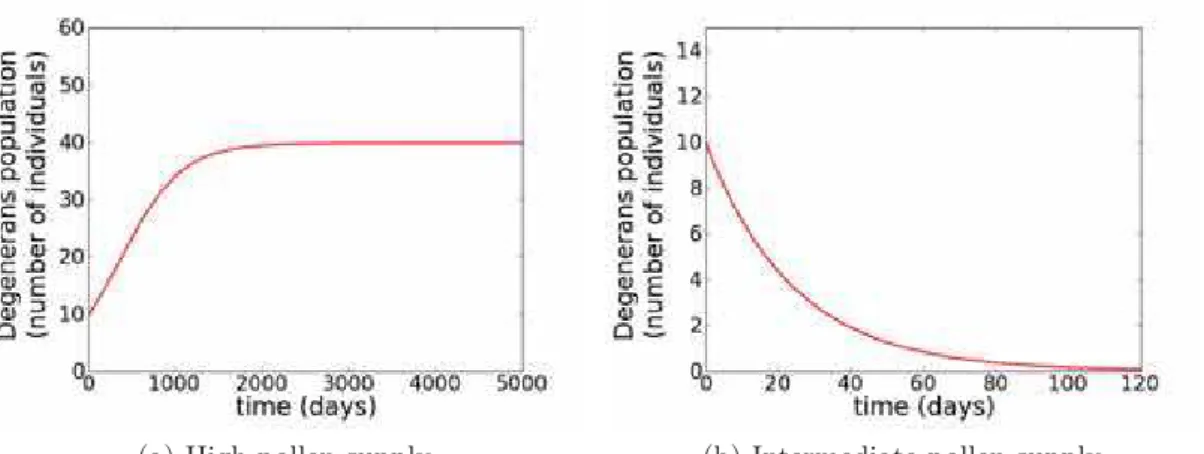
Montserrat et al. [2008] tested the patterns of exclusion along a productivity gradient predicted by IGP theory, in a microcosm experiment. The system was composed of two predatory mite species, Iphiseius degenerans (the IG predator) and Neoseiulus cucumeris (the IG prey), feeding on cattail pollen (the shared resource).
Before studying the dynamics of the complete system, assumptions of the theory were tested. In order to check the abilities of consumers at exploiting resource, preliminary experiments were carried with each competitor alone with pollen. Arenas were supplied twice a week with either4.8x10−3
g (high level) or 8 x 10⁻⁴
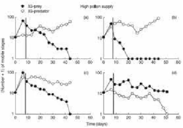
g (intermediate level) of pollen. These resource input rates are, in this experiment, a measure of the environmental productivity. Dynamics of the IG predator and the IG prey for these two resource levels are shown, respectively, in figure 3.1a and 3.1b.
Figure 3.1: Dynamics of the IG prey (figure a) and IG predator (figure b) in the presence of a high (solid lines) and intermediate (dashed lines) pollen supply. This figure was taken from Montserrat et al. [2008].
With high level of resource both consumers seemed to go to a stable equi-librium. However, at the intermediate level only the IG prey persisted, the IG predator went extinct for all replicas. Hence, the IG prey can persist with a smaller amount of resource than the predator, which shows its competitive su-periority. This experimental system then fulfill the prerequisites for coexistence of all three species, and, in addition, the usual IGP pattern, with IG prey domi-nating low productivities, coexistence possible only in intermediate productivities and IG predator dominating high productive environments, is expected.
is scarce). They checked this point by setting an female of I. degenerans with 30 juveniles ofN. cucumeris, with and without an abundant pollen supply. After 24 h, the number of dead juveniles and eggs laid by the female were counted. Results are shown in figure 3.2 (taken from Montserrat et al. [2008]). The number of dead juveniles in the presence or absence of resource does not present significant difference, implying the validity of the premise of intraguild predation in presence of resource. Having observed that premises of theory are met, they proceed to test the predictions of IGP theory.
Figure 3.2: Preliminary tests on the predation pattern of the IG predator. a) The number of dead IG prey juveniles for four different configurations, according to the presence or absence of the IG predator and pollen. b) Daily laid eggs by the IG predator in the presence of the IG prey and pollen, or in the presence of only pollen or only the IG prey.
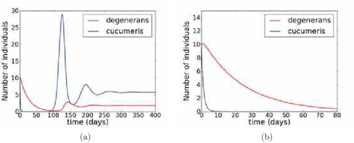
The same amounts of pollen used in the preliminary tests (intermediate and high) were used for the evaluation of the complete system dynamics. Suppression of the prey was observed in the high pollen supply experiments (see figure 3.3). This result agrees with theory if we assume that this is the productivity region of the IG predator dominance.
However, unexpectedly in experiments with intermediate level pollen supply the IG prey was eliminated in five out of six replicates (as shown in figure 3.4). This result is inconsistent with theory, once the IG predator doesn’t persist with the resource alone in this productivity level and, then, it would be expected either coexistence or persistence of only the IG prey.
20 Chapter 3. Tests of the theory
Figure 3.3: Population dynamics of I. degenerans,N. cucumeris and pollen for a high level pollen supply.
4
Transient dynamics in the simple IGP module
Studies on population dynamics have traditionally focused on equilibrium dynam-ics. This tendency can be easily understood due the complexity of the majority of systems of importance in ecology. These systems often present coupled non-linear equations and analytical solutions for the problem can only be found in limited cases. Analysis of stationary states, in turn, has been extensively employed as a powerful tool for assessing analytical results and, in numerous cases, successfully captures important features of real systems.
Yet in many cases, in natura or in laboratory, systems may have not reached equilibrium and analysis of the transient dynamics becomes an important issue [Hastings, 2001, 2004]. This is what happens in many experiments in IGP, in which, due obvious limitations, duration of observations are short relative to the generation time of species involved [Briggs and Borer, 2005].
Care must also be taken when systems present large oscillations during tran-sients, once populations can attain very low levels so that the only reasonable interpretation is that extinction is likely, although stationary states do not pre-dict exclusion of individuals [Hastings, 2001]. As will be shown in this chapter, models for intraguild predation potentially present large oscillations in short-term dynamics. We recall here that IGP theory is based on equilibrium states, then, focusing on transient dynamics, new interpretations for theory can be given.
In the next section, using a simple model for IGP, we analyze the experiment with mites described in the previous chapter.
4.1
Transient dynamics and patterns of exclusion
of mites
Because pollen (the basal resource in the experiments) supply was carried at a constant inflow rate, a chemostat resource growth equation, in the absence of consumers, best resembles experimental conditions. Hence, we propose the following set of differential equations to model the system
dP dt = b
′a′RP +βαN P −m′P (4.1a)
dN
dt = baRN −αP N −mN (4.1b)
dR
dt = µ−φR−aN R−a
′P R, (4.1c)
whereµ is the inflow rate of resources and can be directly obtained from experi-ment, once resource intake was completely controlled. Resource decays at a rate
φ. P and N are, respectively, the population numbers of I. degenerans (the IG predator) and N. cucumeris (the IG prey). The remaining parameters have the same interpretation as in 2.7.
We do not intend to mimic the exact dynamics observed in experiments. Our purpose, however, is to call attention for the fact that transient dynamics in IGP often presents prey populations that attain levels very close to extinction and that, applying these arguments to the experiment of Montserrat et al. [2008], we get an plausible explanation for the unexpected results found on it. Parameters were then estimated using preliminary results from experiment and from van Rijn et al. [2002] (see appendix A), and are shown in table 4.1.
Having fixed parameters, we first checked whether the dynamics of the model for each consumer alone with resource is consistent with observations. That is, if for intermediate pollen supply only N. cucumeris can persist with resource and if at high pollen supply both consumers persist with resource. Simulations are shown in figures 4.1a, 4.1b, 4.2a and 4.2b.
In order to evaluate the dynamics of the complete system, initial conditions were set following those of the experiment. Figure 4.3 shows the population dynamics of the complete system predicted by the model, for high level pollen supply. As verified experimentally, IG predator eliminates the IG prey at this resource level, and this result does not depend on initial conditions (this point is not shown here).
Interesting results appear when we look to intermediate pollen level, in which unexpected outcomes were verified in experiments. A typical dynamics found in simulations for this resource level is shown in figure 4.4a.
4.1. Transient dynamics and patterns of exclusion of mites 25
Table 4.1: Parameters used in simulations.
Parameter value unit
b′ 275 predator/mg
b 275 prey/mg
a′ 0.00037 1 / (predator.day)
a 0.012 1 / (prey.day)
m′ 0.05 1 / day
m 0.05 1 / day
β 0.075 predator/prey
α 0.1 1 / (predator.day)
µ 1.37(high) mg/day 0.229 (intermediate) mg/day 0.0286 (low) mg/day
φ 0.25 1 / day
(a) High pollen supply (b) Intermediate pollen supply
(a) High pollen supply (b) Intermediate pollen supply
Figure 4.2: As in figures 4.1a and 4.1b, but now for N and R (N. cucumeris
and pollen, respectively). IG prey can persist at high and intermediate levels of resource, showing its superiority at exploiting the resource.
4.1. Transient dynamics and patterns of exclusion of mites 27
(a) (b)
Figure 4.4: Dynamics of N. cucumeris and I. degenerans at intermediate pollen supply. a) complete dynamics. b) transient.
this occurs only for large times. If one looks to the short-term dynamics (figure 4.4b), it can be seen that the IG prey population attains very low levels. This deep valley presents high risk of extinction for the IG prey population, and in this simulation its population attains even numbers less than the unity (which is, of course, unrealistic for a real population). Hence, instead of looking to stationary states, in which usual theory is based, we reinterpret results assuming that extinction occurred during transient. Interpreting results in this form we get exactly what was found in experiments, in which, for most of repetitions, it was observed IG prey elimination followed by the IG predator decline (figure 3.4).
Transient dynamics, as opposed to asymptotic outcomes, can be strongly af-fected by changes on the initial conditions. We integrated the model with the same initial conditions in the experiments (not shown) and the qualitative results of figure 4.4b didn’t change.
5
IGP and stage structure
In the previous chapters, we introduced models for IGP in which the hole popula-tion, regardless of size and age of individuals, was characterized into only one big class. Nevertheless, stage structure can play an important role in IGP. Different stages may differ greatly in feeding abilities and in their intra and inter-specific interactions.
Mylius et al. [2001] included stage structure of consumers into models for IGP and studied its implication for the dynamics. Two distinct cases were analyzed, one with stage structure only in the IG prey and the other with stages in the IG predator. In this first case, IG prey population was divided into two classes, adult and juvenile, it was assumed that both classes feed on the basal resource, but only juveniles are preyed by the IG predator (see figure 5.1a). This way, the IG prey has a “stage refugium” in which it is invulnerable to predation. In the other case, the IG predator population presents two stages. Only adult stage can prey and both stages feed on the resource (see figure 5.1b). These two scenar-ios present advantage for the prey and it was believed that these benefits would favor IG prey persistence. Then, these authors assessed outcomes of the models along a productivity gradient, and no great qualitative changes were found, com-pared to the simple IGP module. That is, the usual IGP picture, with the IG prey persisting alone with the resource in low-productive environments, coexis-tence occurring only for intermediate and IG predator dominance in productive environments, still holds in these stage structured systems.
In the next section we extend this analysis and study a system of IGP with stage structure in both consumers.
30 Chapter 5. IGP and stage structure
(a) (b)
Figure 5.1: Scenarios of stage structured IGP systems studied by Mylius et al. [2001]. a) Stage structure appears only in the IG prey, N2 are adults andN1 are
juveniles of the IG prey. b) Stage structure is included only in the IG predator,
P2 and P1 are, respectively, adult and juvenile population of this consumer.
5.1
Stage structure in both consumers
Here we introduce a more general IGP system, in which stage structure appears in both consumers. We consider each consumer presenting two life stages, juvenile and adult, so that benefits for the IG prey, such as non-predatory stage of the IG predator and an invulnerable IG prey stage, operate simultaneously. Differently from the models studied by Mylius et al. [2001], in our model we consider that the juvenile class neither reproduces nor feeds on shared resource. Figure 5.2 shows an scheme of the interactions.
Figure 5.2: System of IGP with stage structure in both consumers. IG predator presents two stages, juvenile and adult, represented by P1 and P2, respectively.
N2 and N1, are the adult and juvenile stage of the IG prey.
5.1.1
The model
dP2
dt =mpP1−dpP2 (5.1a)
dP1
dt =
brparpR+bnpanpN1
1 +hrparpR+hnpanpN1
P2−(dp +mp)P1 (5.1b)
dN2
dt =mnN1−dnN2 (5.1c)
dN1
dt =
brnarnR
1 +hrnarnR
N2−
anpP2
1 +hrparpR+hnpanpN1
N1−(dn+mn)N1 (5.1d)
dR
dt =ρ(K−R)−
arnR
1 +hrnarnR
N2−
arpR
1 +hrparpR+hnpanpN1
P2. (5.1e)
P2 and P1 are the adult and juvenile IG predator populations, respectively.
N2 and N1 correspond to the populations of adults and juveniles of the IG prey,
and R is the shared resource population. Because only adults reproduce, growth terms in equations 5.1b and 5.1d are proportional to adults population, P2 and
N2, only. All feeding relations follow Holling type 2 functional responses, so
that consumption rates saturate when prey numbers become large. Adults of the IG predator feed either on juveniles of the IG prey and on the basal resource, with attack rates anp and arp, respectively. Both juveniles and adults of the IG
predator have a natural mortality rate dp. Juveniles of the IG predator leave
this class by a constant maturation rate mp, and then become adults. The IG
prey feeds on resource only, with attack rate arn. Juveniles and adults of this
consumer die with constant rates dn. And mn is the maturation rate of the IG
prey juveniles. bij is the conversion rate of individuals j when feeding on i and
hij is the handling time of species j for the consumption of i. Finally, resource
presents a semichemostat growth in the absence of consumers,ρis the inflow rate of resources and K is the equilibrium state of resource when no consumers are present.
Equilibrium states
i. Trivial case. P∗
2 =P1∗ = N2∗ = N1∗ = 0, R∗ = 0
R∗ =K;
ii. IG prey and resource state. P∗
2 = P1∗ = 0. N2∗, N1∗ and R∗ = R∗N are
32 Chapter 5. IGP and stage structure
R∗
N =
dn+mn
αrn (5.2a) N∗ 2 = mn dn N∗ 1 (5.2b) N∗ 1 =
dnρ(K −R∗N)(1 +hrnarnR∗N)
arnmnR∗N
, (5.2c)
where
αrn=arn
mn
dn
brn−(dn+mn)hrn
.
From equation 5.2c we see that this state is only positive when K > R∗
N.
This means that for the IG prey to persist with resource the environment must be sufficiently productive.
iii. IG predator and resource state. N∗
2 = N1∗ = 0. P2∗, P1∗0and R∗ =R∗P are
not null
R∗
P =
dp+mp
αrp (5.3a) P∗ 2 = mp dp P∗ 1 (5.3b) P∗ 1 =
dpρ(K−R∗P)(1 +hrparpR∗P)
arpmpR∗P
, (5.3c)
where
αrp =arp
mp
dp
brp−(dp+mp)hrp
.
Note that, without the term corresponding to the consumption of the IG prey by the IG predator, system 5.1 is symmetric according to changes in subscripts and variables denoting IG prey and IG predator. Hence, this sta-tionary state differs from the previous one only by the indices of parameters, which here refer to the IG predator. As for the IG prey, the state with IG predator persisting alone with the resource can only exist for productivities above a threshold, K > R∗
P in this case.
iv. Coexistence of consumers.
arn mn dn αrp αnp
−αrn
arp
anp
−ρhrnarn
R2
+
ρKhrnarn−ρ−arn
mn
dn
αrp
αnp
R∗
P +αrn
arp anp R∗ N R
+ρK = 0, (5.4)
where
αnp =anp
mp
dp
bnp−(dp+mp)hnp
.
The stationary states of consumers are
N∗ 2 = mn dn N∗ 1 (5.5a) N∗ 1 =
(R∗
P −R∗)αrp
αnp (5.5b) P∗ 2 = mp dp P∗ 1 (5.5c) P∗
1 =(R∗−R∗N)αrn
dp
mpanp
1 +hrparpR∗+hnpanpN1∗
1 +hrnarnR∗
. (5.5d)
Stability and states dependence on productivity
Determination of the stability of these points with arbitrary constants demands dispendious calculations and probably results do not assume a compact and easily interpretable form. In order to capture the basic outcome of this system, we parametrized the model using constants used by Mylius et al. [2001]. These are parameters for the interaction between Eurasian perch (IG predator), roach (IG prey) and zooplankton (bottom resource), their values are shown in the table 5.1. For this parameters choice the IG prey is competitively superior, for we have
R∗
P = 24> R∗N = 2.4.
We calculated the stationary states and verified their stability for a range of productivity (K) values, using a routine implemented in Python programming language. This process was carried by first calculating the Jacobian matrix (J) of system 5.1, as a function of K and the values of fixed points, which was done using a package for symbolic computational algebra in python, Sympy [SymPy Development Team, 2009]. For each value of K, the equilibrium points and J
34 Chapter 5. IGP and stage structure
Table 5.1: Parameters used in simulations of model 5.1. Values were taken from Mylius et al. [2001].
Parameter value unit
bnp 0.3 predator/prey
brp 10−
5
predator/resource
brn 10−
5
prey/resource
anp 100 1 / (predator.day)
arp 500 1 / (predator.day)
arn 5000 1 / (prey.day)
hnp 0.11 predator/(day.prey)
hrp 5x 10−
5
predator/(day.resource)
hrn 5x 10−
5
prey/(day.resource)
dp 0.05 1 / day
dn 0.05 1 / day
mp 0.1 1 / day
mn 0.1 1 / day
ρ 0.5 1 / day
K varied resource
of the real part of eigenvalues of J. Figure 5.3 shows the outcomes of the system as a function of productivity. Except for the coexistence region (in orange) we only show stable states.
There is a small region in very low productivities where neither of the con-sumers can persist on the basal resource. This is because the resource available is not enough for consumers growth to suppress their mortality. In this region the stationary state of resource is simply K. Increasing productivity, for K > R∗
N
(numerical verification), IG prey persists alone with resource (states in blue) and its population increases linearly with productivity. For its competitive advantage, the IG prey takes resources to levels that are insufficient for maintenance of the IG predator population, even with the additional nutrition taken from consump-tion of the IG prey. As productivity grows the state IG predator and resource becomes stable, but, as the state IG prey and resource remains stable, it first appears in a short bistable region with exclusion of one of the competitors. Then, still for intermediate productivities, coexistence state becomes stable, solid or-ange lines show stable states, while dashed lines are unstable densities. The state IG predator and resource is also stable for this same region of parameters, and, hence, we have alternative states with either coexistence or IG predator and re-source. Finally, for high productivities the stable state IG predator and resource dominates the dynamics.
36 Chapter 5. IGP and stage structure
with the usual theory and is very similar to results found by Mylius et al. [2001]. Recall, however, that our system structure differs from the one presented by these authors. Then, in order to compare our results, we also studied models with stage structure in only one of the consumers, but that follow feeding relations that we used in equations 5.1 (this point will become clear in the next section).
5.1.2
Both consumers with stages x stage structure in only
one of consumers
If we keep the same features of model 5.1, which means that: when species present stages, only adults feed on resource and reproduce, and that also all feeding relations follow a Holling type 2 functional response, a model with stage structure only in the IG prey can be written in the form
dP dt =
brparpR+bnpanpN1
1 +hrparpR+hnpanpN1
P −dpP (5.6a)
dN2
dt =mnN1−dnN2 (5.6b)
dN1
dt =
brnarnR
1 +hrnarnR
N2−
anpP
1 +hrparpR+hnpanpN1
N1−(dn+mn)N1 (5.6c)
dR
dt =ρ(K−R)−
arnR
1 +hrnarnR
N2−
arpR
1 +hrparpR+hnpanpN1
P. (5.6d)
The IG prey continues here with the advantage of having an invulnerable stage but now there is no non-predatory stage of IG predator. All parameters have the same interpretation as in equations 5.1.
In the case where stages appear only in the IG predator, equations are
dP2
dt =mpP1−dpP2 (5.7a)
dP1
dt =
brparpR+bnpanpN
1 +hrparpR+hnpanpN
P2−(dp+mp)P1 (5.7b)
dN dt =
brnarnR
1 +hrnarnR
N− anpP2
1 +hrparpR+hnpanpN
N −dnN (5.7c)
dR
dt =ρ(K−R)−
arnR
1 +hrnarnR
N − arpR
1 +hrparpR+hnpanpN
P2. (5.7d)
A non-predatory stage of the IG predator in this case decreases predation pressure on the IG prey, and no invulnerable stage is present.
(a) Stage structured IG prey. (b) Stage structured IG predator.
Figure 5.4: Equilibrium states along a productivity gradient for: a) model 5.6, with stage structure in the IG prey only, and b) model 5.7, with stage structure in the IG predator only.
Comparing figures 5.4a and 5.4b with figure 5.3 we see that the productivity range in which the state IG prey and resource is stable is greater when we in-clude stages in both consumers. When stages appear in both consumers the two favorable factors enjoyed by the IG prey sum, reducing both the number of IG prey available for consumption and the number of potential predators. Hence, invasion of the IG predator requires greater productivities, once higher amounts of the alternative resource can then maintain its population. Coexistence region size does not differ greatly between the IG predator stage structured model and the model with stages in both consumers. What happens, nevertheless, is that in the latter, for this set of parameters, coexistence appears only in a bistable region.
5.1.3
Lifetime fractions
The lifetime spend in the consumers juvenile stage depends on mortality rates in this stage as well as on the maturation rates, in a way that (di +mi)−
1
is a measurement of the characteristic juvenile lifetime (index iindicates the IG prey or the IG predator). Adult lifetime, in turn, depends only on its mortality rate andd−1
i is a characteristic lifetime in this stage. We can then define the parameter
38 Chapter 5. IGP and stage structure
τi =
di
di+mi
.
Figures 5.5a and 5.5b show how system behaves along different productivities and lifetime fractions.
(a) (b)
Figure 5.5: Phase portrait for different combinations of: a)K and the vulnerable IG prey lifetime fraction (τN), b)K and the nonpredatory lifetime fraction (τP).
In figure 5.5a all parameters other than K and mn were kept constant at
their values in table 5.1. State (or states) attainable by the system for different combinations of parameters K and τN are indicated in each delimited regions
of the figure. Again stability of states were found computationally using Python programming language, following similar processes and packages described earlier. As in figure 5.5a, figure 5.5b shows the possible states for combinations ofK and
τP.
When the IG prey spends most part of its life in the invulnerable stage (low
τN in figure 5.5a) it dominates the system, for it be the best competitor and in
this region of space predation pressure is low. As its vulnerable lifetime increases two effects operates simultaneously, the most immediate one is that, for spending more time vulnerable, predation pressure is increased and its persistence becomes limited to the low-productive region. The other is that once we are considering only adults reproduce, as time spend in the juvenile stage is increased less adults are “being generated” and also, consequently, less newborn individuals. Hence, persistence of the IG prey is negatively affected by this factor. These two effects operating generate the abrupt phase transition seen in the figure, where above some critical value ofτN the state IG prey and resource is not feasible for any K
In figure 5.5b, for low non-predatory lifetime fraction of the IG predator it can suppress the IG prey in high productivities, as it is expected in usual models for IGP. However as its lifetime in the non-predatory stage increases, predation pressure on the IG prey is reduced, increasing productivity range in which IG prey can persist. For high τP, predation is very weak, and also less reproductive
predator individuals are present, making this region favorable for the IG prey persistence. Hence, this consumer dominates the right most region of this figure. The great potential for exclusion of one of consumers in models for IGP has long been attributed to the absence of age structure in these models [Polis and Holt, 1997]. Nevertheless, inclusion of stages in consumers, the way it is done in this work, does not favor coexistence. Stage structure induce asymmetrical benefits in the consumers, given that only the IG prey is favored. And, although the region in which the IG prey can persist with resource increases, exclusion of one of consumers continues being the more likely state attainable.
6
Reciprocal IGP in stage structured systems
The presence of reciprocal IGP in systems in which individuals present different stages of development is a common trait [Polis and Holt, 1992; van der Hammen et al., 2010]. In this case predation often occurs from adult consumers on juvenile stages of the opponent. Yet, little is known about the implications of this feature on the dynamics of IGP.
We studied, through mathematical modeling, a system of IGP presenting this symmetry in predation between consumers. The structure of interactions is the same as that showed in the previous chapter, but here both consumers prey on each other. Figure 6.1 shows a scheme of interactions.
Figure 6.1: Scheme of interactions considered in this chapter. Two consumers, P and C, compete for resource R and also engage in reciprocal predation.
Note that now we do not have the notion of a IG predator and a IG prey, for
both consumers can prey on their competitor. We still bear, however, the same nomenclature of previous chapters, P and N for consumers. P and N present two stages, juvenile and adult. Adults (index 2) feed on the basal resource and on the juvenile stage (index 1) of their competitors. Juveniles give rise to adults and only then they can reproduce.
6.1
Equations representing the system
The following set of differential equations were used as a representation of these interactions
dP2
dt = mpP1 −dpP2 (6.1a)
dP1
dt = (brparpR+bnpanpN1)P2−apnN2P1−(dp+mp)P1 (6.1b) dN2
dt = mnN1−dnN2 (6.1c)
dN1
dt = (brnarnR+bpnapnP1)N2−anpP2N1−(dn+mn)N1 (6.1d) dR
dt = ρ(K−R)−arnRN2−arpRP2. (6.1e)
For simplicity, we used linear functional responses rather than saturating. All parameters, except apn and bpn, have the same interpretation as in model 5.1.
bpn is the conversion efficiency of consumer N in generating newborn individuals
from consumption of P, and apn is the attack rate of N on P.
6.1.1
Equilibrium points
i) Trivial state, P∗
2 =P1∗ =N2∗ =N1∗ = 0.
R∗ =K;
ii) Only consumer N and resource state, P∗
2 =P1∗ = 0.
R∗
N =
(dn+mn)dn
brnarnmn
(6.2a) N∗ 2 = mn dn N∗ 1 (6.2b) N∗ 1 =
ρdn(K −R∗N)
arnmnR∗N
6.1. Equations representing the system 43
iii) Only consumer P and resource state, N∗
2 =N1∗ = 0.
R∗
P =
(dp +mp)dp
brparpmp
(6.3a) P∗ 2 = mp dp P∗ 1 (6.3b) P∗ 1 =
ρdp(K−R∗P)
arpmpR∗P
; (6.3c)
iv) Coexistence state.
Defining the constants
γn =
bnpanp−apn
mn
dn
dp
mp
/brparp
and
γp =
bpnapn−anp
mp
dp
dn
mn
/brnarn,
R∗ is given by the solutions of equation
arnmn
dnγn
+arpmp
dpγp
R2
+
−ρ− arnmn
dnγn
R∗
P −
arpmp
dpγp
R∗
N
R
+ρK = 0. (6.4)
N∗ 2 = mn dn N∗ 1 (6.5a) N∗ 1 =
(R∗
P −R∗)
γn (6.5b) P∗ 2 = mp dp P∗ 1 (6.5c) P∗ 1 =
(R∗
N −R∗)
γp
6.2
States dependence on environmental
produc-tivity
This system was also parametrized with constants of table 5.1. bpn was assumed
as being equal to bnp and apn was varied. With this parametrization N
contin-ues being the best competitor and in addition, here, has also the advantage of attacking the weaker. Figures 6.2a-d show the system outcomes alongK in order of increasing apn.
(a)apn= 0. (b)apn= 10.
(c)apn= 20. (d)apn= 50.
6.2. States dependence on environmental productivity 45
Figure 6.2a is simply a case without crossed predation and serves as a reference for comparisons. The case of a low defending N is showed in figure 6.2b. Recall that the attack rate of P on N (anp) is 100. At low productivities, as it is
expected, the best competitor-consumer continues dominating the system, once besides being the best competitor, it also attacksP. Productivity range in which
N dominates increases when predation is reciprocal, and continues this tendency as apn is augmented (see figure 6.2c). Hence, the more N attacks, the more
difficult is for P to invade a system with N and R. Coexistence region seems to increase with increasingapn, although region with only coexistence shrinks and a
great extension of coexistence stable states are in a bistable region with states of the consumerP and R also being possible. And finally, above some critical value of apn coexistence region vanishes, giving place to alternative states of P +R or
N +R, which dominate productive environments.
Coexistence in IGP occurs due the presence of trade-offs in the consumption abilities of consumers [Amarasekare, 2010]. The IG prey, in usual IGP system, compensates its non-predatory behaviour on the IG predator by being the best competitor. The IG predator, in turn, though not being superior at exploiting the shared resource, can prey on its competitor. For some range in productivity, even it being sometimes small, there is a balance in these abilities and coexistence is possible. In reciprocal IGP both consumers have abilities of consuming basal resource as well as their competitors, and now coexistence will depend on the strength of interactions. In figure 6.2, for example, while N attacked P weakly, coexistence regions were observed. However, as strength of these attacks increase, the balance in abilities is broken and gives place to a large region of bistability, where one of consumers is excluded.
These results become clearer when we look to a phase portrait indicating states as a function of productivities and the attack rate of N on P (apn), see
figure 6.3. As pointed earlier, for low defended N this system is very similar to the asymmetrical case. However, when attack rate ofN is nearly20%ofP attack rate, coexistence is absent and a large bistable region appears. While in usual IGP one consumer (the IG predator) dominates high-productive environments, when predation is reciprocal for a great range of attack rates (apn) two states
are possible, either N +R or P +R. And even when N attack rate is close, or greater, than P attack rate on N, this picture remains the same. That is, a weaker competitor and also a weaker predator (P, when apn > anp) can still
persist with resource alone, when N is rare, but can not invade the state N and
R.
This picture illustrates well how system behaves as we change predation strengths of one consumer on the other, extending from a weak defending N
to the most symmetrical case where both competitors attack each other with the same strength. Another interesting question to address is the dependence of states according to changes in the abilities of resource consumption. Having fixed
states as a function of these parameters are shown in figure 6.4.
For low attack rates of P on R, N, besides attacking P, is much stronger competitor. This way, great attack rates of P on N are required for it persist and make a region of coexistence. Increasing arp competition becomes more