www.earth-surf-dynam.net/4/407/2016/ doi:10.5194/esurf-4-407-2016
© Author(s) 2016. CC Attribution 3.0 License.
Modeling long-term, large-scale sediment storage using
a simple sediment budget approach
Victoria Naipal1, Christian Reick1, Kristof Van Oost2, Thomas Hoffmann3, and Julia Pongratz1 1Department of Land in the Earth System, Max Planck Institute for Meteorology, Hamburg, Germany 2Université catholique de Louvain, TECLIM – Georges Lemaître Centre for Earth and Climate Research,
Louvain-la-Neuve, Belgium
3Department of Geography, University of Bonn, Bonn, Germany
Correspondence to:Victoria Naipal ([email protected])
Received: 22 December 2015 – Published in Earth Surf. Dynam. Discuss.: 18 January 2016 Revised: 14 April 2016 – Accepted: 3 May 2016 – Published: 20 May 2016
Abstract. Currently, the anthropogenic perturbation of the biogeochemical cycles remains unquantified due to the poor representation of lateral fluxes of carbon and nutrients in Earth system models (ESMs). This lateral transport of carbon and nutrients between terrestrial ecosystems is strongly affected by accelerated soil erosion rates. However, the quantification of global soil erosion by rainfall and runoff, and the resulting redistribution is missing. This study aims at developing new tools and methods to estimate global soil erosion and redistribution by presenting and evaluating a new large-scale coarse-resolution sediment budget model that is compatible with ESMs. This model can simulate spatial patterns and long-term trends of soil redistribution in floodplains and on hillslopes, resulting from external forces such as climate and land use change. We applied the model to the Rhine catchment using climate and land cover data from the Max Planck Institute Earth System Model (MPI-ESM) for the last millennium (here AD 850–2005). Validation is done using observed Holocene sediment storage data and observed scaling between sediment storage and catchment area. We find that the model reproduces the spatial distribution of floodplain sediment storage and the scaling behavior for floodplains and hillslopes as found in observations. After analyzing the dependence of the scaling behavior on the main parameters of the model, we argue that the scaling is an emergent feature of the model and mainly dependent on the underlying topography. Furthermore, we find that land use change is the main contributor to the change in sediment storage in the Rhine catchment during the last millennium. Land use change also explains most of the temporal variability in sediment storage in floodplains and on hillslopes.
1 Introduction
Soil erosion by rainfall and the resulting soil redistribution in a landscape play an important role in the cycling of soil carbon and nutrients in ecosystems (Van Oost et al., 2007). On the one hand, vertical fluxes of carbon and nutrients occur due to either mineralization on eroded landscapes and during sediment transport or sequestration in depositional sites (Lal, 2003, 2005; Van Oost et al., 2007; Quinton et al., 2010). On the other hand, significant lateral fluxes of soil carbon and nutrients can take place when soil redistribution promotes the
lateral transport of these elements in and between terrestrial ecosystems (Van Oost et al., 2007; Quinton et al., 2010).
erosion being a net source (Lal et al., 2004) or a net uptake or sink of CO2(Stallard, 1998; Van Oost et al., 2007).
However, data on global soil erosion and redistribution are scarce to non-existent. There exist several modeling ap-proaches to estimate global soil erosion rates (Yang et al., 2003; Ito, 2007; Montgomery, 2007; Doetterl et al., 2012; Naipal et al., 2015). These modeling approaches mainly ad-dress the soil detachment process only, and do not simulate soil redistribution by ignoring processes such as sediment de-position and transport. There is, to our knowledge, no spa-tially explicit model that can simulate soil redistribution on large spatial scales, for the past, present and future. The lack of such kind of large-scale models on soil redistribution sub-stantially limits the understanding of the interaction of soil erosion and redistribution with the global biogeochemical cy-cles. Therefore, the net global effect of accelerated soil ero-sion on the vertical and lateral fluxes of soil carbon and nu-trients is still unknown.
Consequently, the land components of Earth system mod-els (ESMs), which are the main tools to investigate the ter-restrial carbon cycle and the carbon flux between soil and the atmosphere, ignore the lateral carbon fluxes associated with soil redistribution (Regnier et al., 2013; Van Oost et al., 2012). Therefore, they miss an important aspect of the cou-pling between land and the ocean. In addition, omitting soil erosion from soil organic carbon cycling schemes results in uncertainties in the soil organic carbon flux with various im-plications (Chappell et al., 2015). Including soil redistribu-tion processes in ESMs is thus essential to create the pos-sibility to study the full interactions and feedbacks between the soil and atmosphere with respect to the global biogeo-chemical cycles, and to better understand the anthropogenic perturbation of these cycles.
The holistic understanding of the interaction and linkages between soil erosion, deposition and transport can be ad-dressed using the sediment budget approach (Walling and Collins, 2008). Slaymaker (2003) defined the sediment bud-get as a mass balance where the mass of sediments is con-served in the considered system so that the net increase in sediment storage is equal to the excess of inflow over outflow of sediment. However, long-term large-scale sediment bud-gets are very scarce to non-existent. Sediment budbud-gets that have been constructed previously range from small catch-ments (Verstraeten and Poesen, 2000; Walling et al., 2001) to large river catchments (Milliman and Meade, 1983; Ludwig and Probst, 1998; Syvitski et al., 2003; Slaymaker, 2003). However, these sediment budgets are usually for present day only as they are mostly based on measurements using meth-ods such as sediment tracing or fingerprinting. Also, most of these studies only focus on the sediment delivery from a catchment. They are thus of limited use for assessing the spatial distribution of sediment sources and storage or in pre-dicting long-term sediment yields. Considering explicitly the spatial distribution of these variables within a catchment is essential not only for a proper land management strategy to
combat land degradation but also for a detailed assessment of how soil erosion and redistribution interact with the carbon and nutrient cycles. Furthermore, it is also essential to con-sider long-term sediment budgets, as they can provide essen-tial information on the forces behind sediment, carbon and nutrient fluxes in a catchment such as human activities and climate change.
There exist different spatial models of suspended sediment flux that also consider the soil redistribution or sediment dy-namics in a catchment (Merritt et al., 2003; de Vente and Poesen, 2005; Ward et al., 2009). However, many of them are developed to simulate single events or require input data that are not available for large spatial scales (Wilkinson et al., 2009). There are also partly empirical models which can op-erate on the catchment scale such as the WATEM/SEDEM model and the suspended sediment model from Wilkinson et al. (2009). The WATEM/SEDEM model is used to pre-dict hillslope sediment storage and sediment yield (de Moor and Verstraeten, 2008; Nadeu et al., 2015), while the sus-pended sediment model also simulates some other processes such as floodplain deposition, gully and riverbank erosion. However, these models are not compatible for a global-scale application as they require parameters for which data are not available on a global scale. In addition, these types of mod-els also need to be calibrated to measured sediment yields of the studied area (Van Rompaey et al., 2001). Pelletier (2012) proposed a global applicable model for long-term suspended sediment discharge, where he used various environmental controlling parameters to simulate soil detachment and sed-iment transport. However, in his study he mainly focuses on the sediment discharge and delivery of catchments and his model does not take into account the full dynamics of sed-iment in a catchment, which would also include the spatial distribution of sediment deposition and storage in the dif-ferent reservoirs of a catchment. Additionally, he does not consider land use change and thus his approach is limited to natural catchments only.
2 Methods
2.1 Basic model concept
The main purpose of the sediment budget model presented here is to estimate large-scale, long-term floodplain and hill-slope sediment storage and lateral fluxes of sediment. The model should, therefore, be spatially explicit and capable of estimating erosion, deposition and sediment transport pro-cesses. For this purpose we will use a grid-cell-based ap-proach. Compatibility of this new model with ESMs is im-portant for a future extension of the model to include the carbon and nutrient cycling. Furthermore, it is essential to distinguish between floodplain and hillslope systems due to the distinct differences in sediment dynamics between these systems (Hoffmann et al., 2013). Human activities usually lead to a stronger increase in sediment deposits on hillslopes compared to floodplains, and an overall decreased export of sediment out of a catchment, despite increased soil ero-sion (de Moor and Verstraeten, 2008). In this way, sediments stored in floodplains and on hillslopes over long timescales can significantly delay or alter the human-induced changes to the carbon and nutrient cycles (Hoffmann et al., 2013).
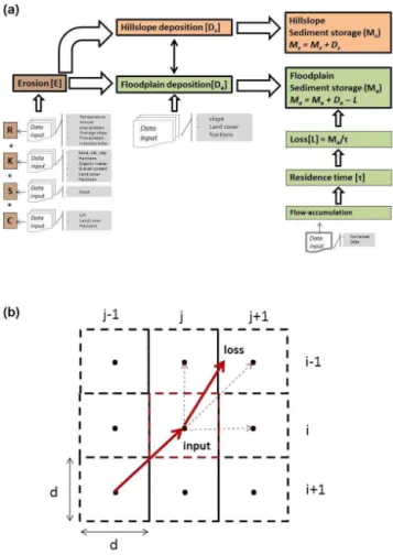
Before we can define a model that satisfies the above-mentioned conditions we have to make some basic assump-tions. First, as it is difficult to disentangle the floodplains and hillslopes in available soil data sets, we assume that each grid cell contains both a hillslope and a floodplain reservoir. When estimating large-scale sediment storage with the aim of predicting the effects of soil redistribution on the biogeo-chemical cycles, the focus is to get the large-scale spatial patterns right, rather than accurate numbers for the sediment storage and fluxes. Second, we assume that the sediment de-position and transport behave differently between the flood-plain and hillslope reservoirs on the timescale of the last mil-lennium. Third, erosion is considered to mainly take place on hillslopes, where part of the eroded sediment is directly transported from hillslopes and deposited in the floodplains. The underlying model framework (Fig. 1a) that consists of the erosion, deposition and sediment transport modules is based on the sediment mass-balance method. The change in sediment storage (M) within a certain unit of time and space is given by the difference between sediment input and sediment output (Slaymaker, 2003). For sediment stored in floodplains (Ma), this leads to
dMa
dt =Da−L. (1)
Here, Da is the sediment deposition rate in floodplains,
and L is the sediment loss. Equation (1) can be seen as a representation of the net soil redistribution flux, and is ap-proximated by the following as function of time:
dMa
dt =Da(t)−k×Ma(t), (2)
Figure 1.Model scheme(a)with multiple flow routing(b).
whereDa(t) is the time-dependent input rate in the model,
which is independent ofMa(t),k×Ma(t) is the loss term of
the floodplain reservoir, andk is the specific rate for flood-plains.
The specific rate is the inverse of the residence time (1/τ) for floodplain sediment.τ is defined as the time (in years) a soil particle stays in the floodplain reservoir of a certain grid cell. Here, we assume that τ is independent of time for timescales in the order of a few thousands of years. We also assume that τ is increasing exponentially with catch-ment area or weighted flow accumulation (FlowAcc):
τ=e
(FlowAcc−aτ)
bτ , (3)
aτ andbτ are the adjustment parameters of the model that
the system capable of storing sediment for long time peri-ods. The opposite is true for small catchment areas, where the connectivity is usually high, resulting in short residence times for sediment (Hoffmann, 2015).
Dacan be defined as a certain fraction of the erosion rate
(E). In this way Eq. (2) can be rewritten as
dMa
dt =f(t)×E(t)− Ma(t)
τ , (4)
wheref is the dimensionless floodplain deposition fraction ranging between 0 and 1.
E (t ha−1year−1) is computed according to the adjusted Revised Universal Soil Loss Equation (RUSLE) model (Naipal et al., 2015), which computes annual averaged rill and inter-rill erosion rates and is formulated as a product of a a slope steepness factor (S, dimensionless), a rainfall erosivity factor (R, MJ mm ha−1h−1year−1), a land cover factor (C, dimensionless), and a soil erodibility factor (K, t ha h ha−1MJ−1mm−1):
E=S×R×C×K. (5)
The underlying RUSLE model stems from the original Universal Soil Loss Equation (USLE) model developed by USDA (USA Department of Agriculture), which is based on a large set of experiments on soil loss due to water erosion from agricultural plots in the United States (Renard et al., 1997). These experiments covered a large variety of agri-cultural practices, soil types and climate conditions, making it a potentially suitable tool on a regional to global scale. Although RUSLE was originally developed for agricultural land, model parameters for other land cover types such as forest and grassland have also been estimated using obser-vational data (Dissmeyer and Foster, 1981; Millward and Mersey, 1999; Lu et al., 2004).
In the adjusted RUSLE model, as presented above, the ef-fects of the slope length (L factor) and support practice (P factor) are excluded. In the original RUSLE model (Renard et al., 1997), these factors are part of the model; however, on a large to global scale there are too few data available on these factors. Including them in the model would only result in additional uncertainties, and we try to keep the model sim-ple so as to be able to capture and quantify the main processes and drivers behind large-scale sediment mobilization. We do, however, agree that leaving these two factors out could intro-duce some biases in erosion rates, especially in agricultural areas.
f is calculated by a simple growth function where deposi-tion is a funcdeposi-tion of the average percent topographical slope (θ) and the main land cover type in a grid cell:
f =af×e
(
bf× θ
θmax )
, (6)
whereaf andbf are adjustment parameters that relatef to
the average slope depending on the land cover type andθmax
is the maximum percent slope. According to Eq. (6), an in-crease in the overall average slope of a grid cell leads to a larger transport of eroded soil from the hillslopes to the plains, leading to an increased deposition rate to the flood-plain reservoir of that specific grid cell. Hereby, we assume the increase inf to be exponential.
The effect of the land cover type onf in our model rep-resents mainly the interaction of the landscape connectiv-ity with sediment transport. The connectivconnectiv-ity of a natural landscape, consisting out of mainly forest, is largely based on the vegetation density and morphological structures (Gu-miere et al., 2011; Bracken and Croke, 2007). In crop and grassland, however, the landscape connectivity is strongly affected by anthropogenic structures. Several recent studies (Hoffmann et al., 2013; de Moor and Verstraeten, 2008; Gu-miere et al., 2011) show that these anthropogenic structures and activities reduce the sediment transport from hillslopes to the floodplains. In this way, the stored hillslope sediment is disconnected from the fluvial system on timescales of 100 to a few 1000 years. Based on this, we assume in our model that for crop and grassland the sediment connectivity is disturbed. A disturbed sediment connectivity will result in a larger frac-tion of eroded soil that remains on the hillslopes compared to the fraction that flows along the hillslopes and is deposited in the floodplains. For natural landscapes we assume a better sediment connectivity, meaning that an equal or larger frac-tion of the eroded soil will be deposited in the floodplains compared to the fraction that remains on the hillslope. Here we ignore morphological conditions that can cause discon-nectivity in the landscape.
After calculating erosion and deposition, the sediment is transported between grid cells based on the multiple flow sediment routing scheme such as presented by Quinn et al. (1991) (Fig. 1b). In the multiple flow routing scheme the weight (W, dimensionless), which specifies the part of the flow that comes in from a neighboring grid cell, is calculated as
Wk,l(i, j)=
θk,l(i, j)×ck,l(i, j)
P1
k,l=−1
θk,l(i, j)×ck,l(i, j)
, (7)
wherecis the contour length and is 0.5 in the cardinal direc-tion and 0.354 in the diagonal direcdirec-tion. (i, j) is the grid cell in consideration whereicounts grid cells in the latitude di-rection andjin the longitude direction.i+kandj+lspecify the neighboring grid cells, wherekandl can be−1, 0 or 1. θis calculated here as
θk,l(i, j)=
h(i, j)−hk,l(i, j)
d , (8)
wherehis the elevation in meters derived from a digital ele-vation model anddis the grid size in meters.
each time steptas
Ma(i, j, t+1)= (9)
Ma(i, j, t)+
f(i, j, t+1)×E(i, j, t+1)−Ma(i, j, t)
τ(i, j)
+
1
X
k,l=−1
M
a k,l(i, j, t)
τk,l(i, j)
×Wk,l(i, j)
.
For hillslopes the change in sediment storage is assumed to be equal to the input rate (Eq. 10), because we assume that the stored hillslope sediment has an infinite residence time on the timescale of the last millennium in accordance with the study of Hoffmann (2015). This means that the hillslope sediment storage will increase linearly with time (Eq. 11). The hillslope sediment deposition rate (Dc) is here defined
as the remaining part of the eroded soil that has not be been transferred to the floodplain directly (1−f). The equations for the hillslope sediment storage rate (Mc, t ha−1year−1) are
represented by
dMc
dt =Dc=(1−f(t))×E(t), (10) and
Mc(i, j, t+1)= (11)
Mc(i, j, t)+(1−f(i, j, t+1))×E(i, j, t+1).
The modeling approach as presented by the equations above focuses on the net soil redistribution by separately modeling the main processes of soil redistribution, which are erosion, deposition and transport. In the following para-graphs we will show how this dynamical modeling approach performs when applied on the Rhine catchment.
2.2 Model implementation and parameter estimation The resolution of the sediment budget model is 5 arcmin. The main reason for choosing this particular model resolution is based on the assumption that this resolution is optimal when considering that each grid cell contains a floodplain and hill-slope fraction. Here, a higher resolution could lead to cases where this assumption is not met. Also, the 5 arcmin reso-lution fits well with the resoreso-lution of the adjusted RUSLE model.
The sediment budget model uses climate and land cover data from simulations of the Max Planck Institute Earth Sys-tem Model (MPI-ESM) that have been performed under the Coupled Model Intercomparison Project Phase 5 (CMIP5) framework (Hurrell and Visbeck, 2011; Taylor et al., 2009). As these data were given at a resolution of approximately 1.875◦, we had to downscale the data to the resolution of the sediment budget model. For the period AD 1850–2005 three ensemble members from MPI-ESM (r1i1p1, r2i1p1, r3i1p1) were available, while for the period AD 850–1850 only one
ensemble member (r1i1p1) was available. These data existed on a 6-hourly, monthly or yearly time step for the last mil-lennium.
Calculation of soil erosion according to the adjusted RUSLE model is mostly based on the methods presented in the study of Naipal et al. (2015). However, the calculation of theRandCfactors had to be adapted due to the very coarse resolution of the data from MPI-ESM or the lack of data on certain parameters of the model. A detailed description of erosion estimation with the adjusted RUSLE model in com-bination with data from the MPI-ESM model is presented in the Supplement.
Additionally, due to the overestimation of erosion rates by the adjusted RUSLE model in the Alps, we defined a mean soil erosion rate of 20 t ha−1year−1for this region based on high-resolution erosion data from Bosco et al. (2008).
We chosef to range between 0.5 and 0.8 for forest, and between 0.2 and 0.5 for crop and grassland. These numbers are based on findings from the study of de Moor and Ver-straeten (2008), where they show a deposition rate in flood-plains that is approximately equal to that on hillslopes be-fore agricultural activities started in the Geul River catch-ment in the Netherlands. However, for present day they show that much more sediment is trapped on hillslopes than is transferred to the floodplains. Based on the chosen ranges forf and Eq. (6) we calculatedaf andbf for forest to be
0.5 and 0.47, respectively, and for crop and grassland to be 0.2 and 0.917, respectively. This means that for low slopes (<±0.2 %) in a forest an equal amount of sediment is de-posited in floodplains as on hillslopes, while for crop and grassland only 20 % of the eroded soil from the hillslopes will reach the floodplains.
The floodplain residence time is made to range between the median and maximum residence time of floodplain sedi-ment in the Rhine catchsedi-ment of 260 and 1500 years, respec-tively. This is in accordance with the residence times derived from observed sediment storage in the Rhine catchment. Fur-thermore, Wittmann and von Blanckenburg (2009) found a residence time of 600 years for floodplain sediments at Rees in the Rhine catchment, which falls in the range of the flood-plain residence times of our study. We used the median and maximum residence times and the maximum flow accumu-lation of the Rhine catchment to determine theaτ andbτ in
Eq. 3. The exact values foraτ andbτ are−922 442.54 and
165 886.77, respectively.
2.3 Criteria for model evaluation
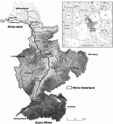
in-Figure 2.The Rhine catchment (Hoffmann et al., 2013).
vestigate the impact of human activities on erosion and sed-iment yields through history. The Rhine catchment (Fig. 2) has a size of∼185 000 km2with a main river channel length of∼1320 km and drains large parts of the area between the European Alps and the North Sea. It has a complex topog-raphy where the elevation ranges between−180 and 1967 m with a mean topographical percent slope of 0.07, where per-cent slopes can go up to 1.2. It consists of two large sedi-mentary catchments (i.e., upper Rhine Graben and the lower Rhine Embayment–southern North Sea Basin) that serve as large floodplain sinks for sediment and some upland areas, such as the Black Forest and the European Alps, that serve as major sediment production areas.
From observed Holocene sediment storage, Hoffmann et al. (2013) derived scaling relationships between sediment storage S (109kg=1 Mt) and catchment area A(km2) for floodplains and hillslopes. They found that for floodplains the sediment storage increases in a non-linear way with catchment area, while for hillslopes this increase is linear. With these scaling relationships, for the first time, a direct comparison is made between the behavior of soil redistribu-tion on hillslopes and in floodplains at large spatial scales. This is an essential difference between hillslopes and flood-plains that large-scale sediment budget models like ours need to capture in order to reliably simulate the spatial distribution of sediment on such a scale. The scaling relationships, given by Eq. (12) for hillslopes and Eq. (13) for floodplains, will be used as a simple validation test for our coarse-resolution sediment budget model.
S=(364±168)106× A
Aref
(1.06±0.07)
(12)
S=(184±24)106×
A
Aref
(1.23±0.06)
(13)
Here,Aref is an arbitrary chosen reference area, in this case 103km2. The observation data contain 41 hillslope and 36 floodplain sediment storage values, derived from a large number of auger and bore holes that are used to measure sed-iment thickness related to human-induced soil erosion.
With the estimated scaling exponents (Eqs. 12 and 13) Hoffmann et al. (2013) showed that, even for large catch-ments (in the order of 105km2), hillslopes store an equal amount of sediment as floodplains. They pointed out that this is a substantial sink that needs to be considered in sediment budgets of large catchments.
Furthermore, Hoffmann et al. (2007) established a Holocene sediment budget for sediments in the floodplains and the delta of the non-Alpine part of the Rhine catchment. They derived sediment thickness of Holocene deposits from borehole data that consist of 563 drillings and available ge-ological maps. This was then multiplied with floodplain ar-eas to calculate floodplain volumes. Sediments on hillslopes were not addressed in this study. A total floodplain sediment mass of 53.5±12.4×10⁹t was found for the whole Rhine catchment, of which 50 % is stored in the Rhine Graben and the delta. The spatial variability in this observed sediment storage in floodplains will be a second validation test for our model.
Finally, Hoffmann et al. (2007) also found an average ero-sion rate of 0.55±0.16 t ha−1year−1for the last 10 000 years, with extreme minimum and maximum values of 0.3 and 2.9 t ha−1year−1. However, Hoffmann et al. (2013) also in-cluded hillslope sediment storage and calculated a total sedi-ment storage of 126±41 Gt for the Rhine catchment, which requires a minimum Holocene erosion rate of approximately 1.2±0.32 t ha−1year−1. This shows that hillslopes are not only the main sources of eroded sediment but can also be major millennial-scale sinks for eroded sediment that comes from agriculture. We will use the average erosion rates from the abovementioned studies as a comparison to the rates de-rived from our sediment budget model.
2.4 Simulation setup
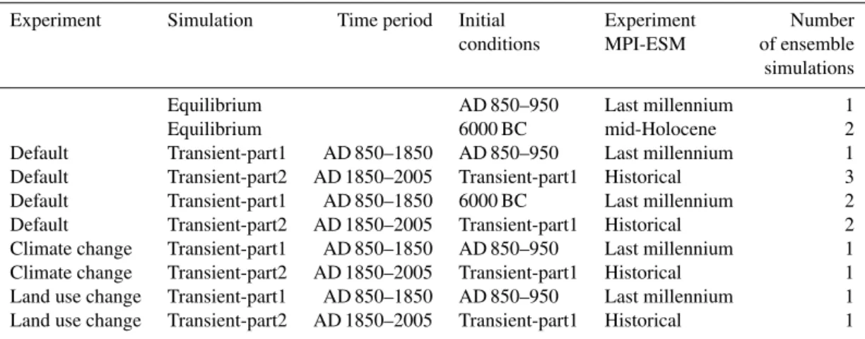
Table 1.Simulation specifications for the application of the sediment budget model on the Rhine catchment. For each experiment with the sediment budget model, the type of simulation (equilibrium or transient), the time period, and the initial conditions on which the simulation is based are given. Furthermore, we also provide the number of simulations we made with the model for a certain type of simulation, and the experiment from MPI-ESM that we used to derive the input data to force the sediment budget model.
Experiment Simulation Time period Initial Experiment Number
conditions MPI-ESM of ensemble
simulations
Equilibrium AD 850–950 Last millennium 1
Equilibrium 6000 BC mid-Holocene 2
Default Transient-part1 AD 850–1850 AD 850–950 Last millennium 1
Default Transient-part2 AD 1850–2005 Transient-part1 Historical 3
Default Transient-part1 AD 850–1850 6000 BC Last millennium 2
Default Transient-part2 AD 1850–2005 Transient-part1 Historical 2
Climate change Transient-part1 AD 850–1850 AD 850–950 Last millennium 1
Climate change Transient-part2 AD 1850–2005 Transient-part1 Historical 1
Land use change Transient-part1 AD 850–1850 AD 850–950 Last millennium 1
Land use change Transient-part2 AD 1850–2005 Transient-part1 Historical 1
into a transient state. In the case of the Rhine catchment the period directly after the Last Glaciation Maximum (LGM) could be of major importance due to strong erosion that was triggered by the retreating ice sheets. From today’s observa-tions on sediment yields or erosion rates we cannot determine when the Rhine catchment was in an equilibrium state. Ad-ditionally, there are no observations of sediment storage be-fore the start of agricultural activities in the Rhine catchment. This poses a problem in simulating and interpreting present-day absolute values of sediment storage and yields with our sediment budget model.
In order to still be able to interpret the simulated results for the Rhine catchment, we will only focus on the change in sediment storage due to land use and climate change since AD 850. Considering mainly the changes induced by external forcing, it is not necessary to know whether the system was in an equilibrium or transient state at AD 850. Based on this reasoning, we use the environmental conditions of the period between AD 850 and 950 to determine the equilibrium state of the model.
In the rest of this study, we will refer to the period between AD 850 and 950 as the “default equilibrium state” that we define based on the mean environmental conditions between AD 850 and 950, while one should keep in mind that this is not the “real” equilibrium state of the catchment. The period AD 850–950 is used here as the equilibrium state due to rea-sons related to data availability, and because human impact in this time period is still small compared to present day.
Hence, our simulation setup structure is generally defined by an equilibrium simulation based on the mean climate and land cover conditions of the period between AD 850 and 950, followed by a transient simulation for the last millennium.
We performed three equilibrium simulations: one based on the mean climate and land cover conditions of the pe-riod AD 850–950, and the two others based on the mean
cli-mate and land cover conditions of the mid-Holocene period (6000 years ago) from the mid-Holocene experiment of the MPI-ESM (Table 1). The reason for performing an equilib-rium simulation for the mid-Holocene period is to investigate how different initial conditions for climate and land cover in-fluence the overall sediment storage change during the last millennium.
In the equilibrium simulations the erosion and deposition rates are kept constant and the model is run with a yearly time step until the total floodplain sediment storage of a catch-ment does not change by more than 1 t year−1. The flood-plain and hillslope sediment storage at equilibrium were then used as a starting point for the transient simulation that cov-ers the period AD 850–2005. In the transient simulation, ero-sion and deposition rates are averaged over time steps of 100 and 50 years, based on the time resolution of the rainfall ero-sivity factor (R) that is part of the erosion module.
Table 2.Summary of regression results of the scaling of sediment storage at the end of the equilibrium and transient simulations. Here we consider only the grid cells that correspond to the observation points from Hoffmann et al. (2013) and fall into the borders of the Rhine catchment. Thervalue is the Pearson correlation coefficient, and the slope and intercept are the scaling parameters.
Floodplains Hillslopes
Slope Intercept rvalue Slope Intercept rvalue
Equilibrium 1.659±0.037 3.123±0.130 0.99 1.085±0.060 6.429±0.180 0.94 Transient ensemble 1 1.198±0.038 3.877±0.133 0.98 1.050±0.064 4.963±0.193 0.93 Transient ensemble 2 1.202±0.038 3.853±0.133 0.98 1.048±0.065 4.971±0.194 0.93 Transient ensemble 3 1.203±0.038 3.85±0.133 0.98 1.048±0.065 4.972±0.194 0.93
Hoffmann et al. (2013) 1.230±0.060 4.450 0.96 1.080±0.070 5.380 0.96
3 Application of the sediment budget model
3.1 Scaling test
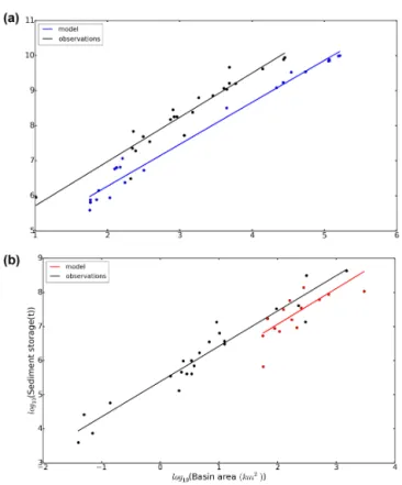
In order to validate the sediment budget model we tested whether the model can reproduce the scaling relationships found by Hoffmann et al. (2013) for the non-Alpine part of the Rhine catchment (Eqs. 12 and 13). For this we chose the grid cells in the Rhine catchment that correspond to the ob-servation points from Hoffmann et al. (2013). Obob-servation points that fell outside the Rhine catchment were not consid-ered. When considering only the selected grid cells and ap-plying the same scaling approach as in the study of Hoffmann et al. (2013), we find average scaling exponents of 1.2±0.04 and 1.05±0.07 for floodplains and hillslopes, respectively (Table 2). These values fall in the range of floodplain and hillslope scaling exponents of 1.23±0.06 and 1.08±0.07, respectively, found by Hoffmann et al. (2013). The uncer-tainty in the scaling exponents is mainly due to the regres-sion, while the uncertainty due to different ensemble simula-tions is very small (Table 2). These results indicate that our model reproduces the characteristic differences in scaling be-tween floodplains and hillslopes as found by Hoffmann et al. (2013) (Fig. 3a and b). One should note that the grid resolu-tion of the model limits the predicresolu-tion of sediment storage to grid points with a catchment area≥102km2.
When considering all the grid cells of the Rhine catch-ment we find a scaling exponent for floodplain storage of 1.33±0.02 (Table 3). This is somewhat higher than the value found when only the selected grid cells are used, which can be explained by the inclusion of grid cells located in the Alpine region of the Rhine catchment. Including the Alpine region thus leads to a stronger gradient in sediment storage and catchment area between the Alps and the Rhine delta. In the Alpine region the model predicts much less sediment storage due to the low residence time and high sediment con-nectivity, while for the Rhine delta the sediment storage is large due to high residence times and low sediment con-nectivity. For hillslope storage the scaling exponent is also slightly higher when including all grid cells in the scaling approach (Table 3). This can also be explained by including the Alpine region, where the model predicts more sediment
Figure 3.Scaling of floodplain(a)and hillslope(b)sediment stor-age from the transient simulation in the non-Alpine part of the Rhine catchment. The black dots and black trend line correspond to the observed sediment storage values from Hoffmann et al. (2013). The colored dots and colored trend line correspond to modeled sediment storage values that correspond to the observation points from Hoff-mann et al. (2013) and fall into the borders of the Rhine catchment.
storage on hillslopes in contrast to the rest of the Rhine catch-ment as a result of high erosion rates.
Table 3.Summary of regression results of the scaling of sediment storage after the equilibrium and transient simulations. Here we consider all grid cells in the Rhine catchment area. Ther value is the Pearson correlation coefficient, and the slope and intercept are the scaling parameters.
Floodplains Hillslopes
Slope Intercept rvalue Slope Intercept rvalue
Equilibrium 1.685±0.015 2.827±0.039 0.80 1.118±0.016 6.327±0.040 0.62 Transient ensemble 1 1.330±0.017 3.406±0.042 0.67 1.111±0.015 4.741±0.039 0.63 Transient ensemble 2 1.332±0.017 3.401±0.042 0.67 1.112±0.015 4.740±0.039 0.63 Transient ensemble 3 1.332±0.017 3.400±0.042 0.67 1.112±0.015 4.741±0.039 0.63
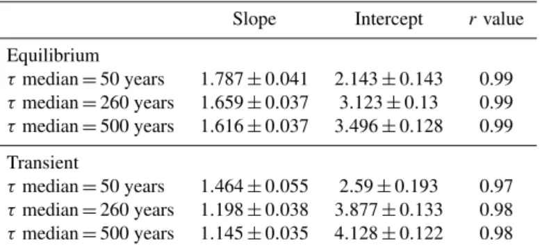
Table 4.Summary of regression results of the sensitivity analysis on floodplain sediment storage scaling. Here we consider only the previ-ously mentioned selected grid cells in the Rhine catchment area.τ is the residence time of floodplain sediment. Thervalue is the Pearson correlation coefficient, and the slope and intercept are the scaling parameters.
Slope Intercept rvalue
Equilibrium
τmedian=50 years 1.787±0.041 2.143±0.143 0.99 τmedian=260 years 1.659±0.037 3.123±0.13 0.99 τmedian=500 years 1.616±0.037 3.496±0.128 0.99
Transient
τmedian=50 years 1.464±0.055 2.59±0.193 0.97 τmedian=260 years 1.198±0.038 3.877±0.133 0.98 τmedian=500 years 1.145±0.035 4.128±0.122 0.98
the catchment. The relatively small difference can be partly attributed to biases in simulated erosion and deposition rates and the floodplain residence times.
Finally, we find that keeping either the climate or land cover constant throughout the last millennium has very little impact on the scaling exponent for floodplain storage. Here, the climate change simulation results in a slightly higher and the land use change simulation in a slightly lower scaling exponent. The different forcings have a stronger impact on the scaling for hillslope storage, as hillslope storage is only dependent on erosion and deposition rates. In the climate change simulation the scaling exponent for hillslope storage increases by 3.8 %, while in the land use change simulation a small decrease of 0.1 % is found. This decrease can result from the fact that most land use change took place in the lower parts of the Rhine catchment resulting in an increased sediment storage there. In contrast, the land use conditions in the Alpine region did not change that rapidly, resulting in a decreased difference in sediment storage on hillslopes be-tween the upper and lower areas of the catchment.
With the above results we show that the scaling relation-ships are a general feature for the entire Rhine catchment and are independent of the selected observation points. As the Rhine catchment is a large catchment with a complex to-pography, this indicates that the scaling relationships might also be applicable for other large river catchments.
3.2 Origin of scaling between sediment storage and catchment area
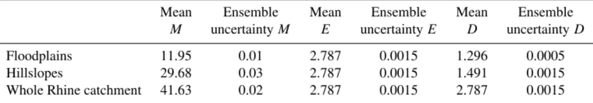
Table 5.Summary of sediment storageM(Gt), erosion (E) and deposition (D) rates in t ha−1year−1, and the related uncertainty ranges for the Rhine catchment for the period AD 850–2005. The uncertainty values represent the range in the mean values due to different ensemble simulations.
Mean Ensemble Mean Ensemble Mean Ensemble
M uncertaintyM E uncertaintyE D uncertaintyD
Floodplains 11.95 0.01 2.787 0.0015 1.296 0.0005
Hillslopes 29.68 0.03 2.787 0.0015 1.491 0.0015
Whole Rhine catchment 41.63 0.02 2.787 0.0015 2.787 0.0015
exponent. However, here the 10-fold change in the residence time leads to a slightly larger change in the scaling exponent. Next, we investigated the dependence of the scaling ex-ponents for floodplain and hillslope storage on erosion. We changed the spatial variability in erosion in the Rhine catch-ment by changing the spatial variability in theRfactor. We increased the R values in the Alpine region and decreased the R values in the rest of the catchment. This results in a larger difference between the sediment storage in small catchment areas and sediment storage in large catchment ar-eas. Although the resulting scaling exponent for floodplain storage is still much higher than the scaling exponent for hill-slope storage, both scaling exponents increase significantly.
For the deposition we find a minor effect on the scaling parameters, which can be neglected.
Overall we find that changing erosion and residence time does not change the basic property of the scaling, which is that floodplain storage increases in a non-linear way with catchment area while hillslope storage increases linearly with catchment area. As the residence time is determined by flow accumulation and flow accumulation determines the spatial variability in floodplain sediment storage, we expect that the scaling parameters for floodplain sediment storage are also mainly determined by flow accumulation. Erosion is mainly determined by the slope, and slope determines the spatial variability in hillslope sediment storage. Therefore, we ex-pect that the slope determines the scaling parameters for hill-slope sediment storage. Based on this we argue that the scal-ing for both floodplain and hillslope storage is an emergent property of the model and that the scaling parameters are controlled by the underlying topography.
3.3 Last millennium sediment storage
We estimate an average soil erosion rate of 2.8±
0.002 t ha−1year−1 for the last millennium for the entire Rhine catchment. We find that this value is twice as high as the 1.2±0.32 t ha−1year−1, which was estimated as the minimum average soil erosion rate for the Holocene by Hoff-mann et al. (2013).
The average soil erosion rate for the last millennium re-sults in a mean floodplain and hillslope sediment storage change for the last millennium of 11.95±0.01 and 29.68±
0.03 Gt, respectively (Table 5). Altogether, floodplain and
hillslope storage result in 41.63±0.02 Gt of sediment, which can be considered as the contribution of climate and land use change to sediment storage in the last millennium. It is, how-ever, hard to say what the range in the change of sediment storage should be for this period, as there are no related stud-ies for this specific time period. The total sediment storage we find is lower than the total Holocene sediment storage of 126±41 Gt found by Hoffmann et al. (2007) for the Rhine catchment. This is logical as we consider only the last mil-lennium and not the past 7500 years as in the study of Hoff-mann et al. (2007). Our results show that the sediment stor-age of the last millennium forms 25 to 50 % of the total sed-iment storage of the last 7500 years. This indicates that the average sediment storage rate during the last millennium is higher than the average rate during the last 7500 years. This also supports the findings from previous studies (Bork, 1989; Notebaert et al., 2011), which show that land use change has a significant and long-term impact on erosion and sediment mobilization.
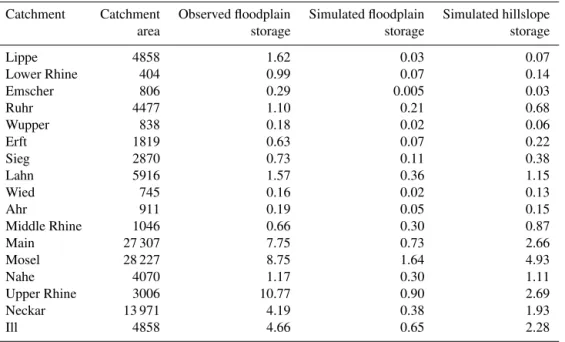
Table 6.Observed versus simulated sediment storage (Gt) for Rhine sub-catchments. The sub-catchment area is given in km2. Data on the observed sediment storage are taken from Hoffmann et al. (2007).
Catchment Catchment Observed floodplain Simulated floodplain Simulated hillslope
area storage storage storage
Lippe 4858 1.62 0.03 0.07
Lower Rhine 404 0.99 0.07 0.14
Emscher 806 0.29 0.005 0.03
Ruhr 4477 1.10 0.21 0.68
Wupper 838 0.18 0.02 0.06
Erft 1819 0.63 0.07 0.22
Sieg 2870 0.73 0.11 0.38
Lahn 5916 1.57 0.36 1.15
Wied 745 0.16 0.02 0.13
Ahr 911 0.19 0.05 0.15
Middle Rhine 1046 0.66 0.30 0.87
Main 27 307 7.75 0.73 2.66
Mosel 28 227 8.75 1.64 4.93
Nahe 4070 1.17 0.30 1.11
Upper Rhine 3006 10.77 0.90 2.69
Neckar 13 971 4.19 0.38 1.93
Ill 4858 4.66 0.65 2.28
Figure 4.Observed vs. simulated floodplain sediment storage for Rhine sub-catchments. The values are in percent (actual storage di-vided by the sum times 100). Data on the observed sediment storage are taken from Hoffmann et al. (2007). RMSE is the root-mean-square error.
sheets, for example, can produce a lot of sediment that is not captured by our model. In this way the total stored sediment in the catchment could be underestimated. Furthermore, it is likely that our model is too coarse for an accurate represen-tation of floodplain storage for the Mosel due to the highly complex topography of this sub-catchment.
For hillslope sediment storage we find a similar spatial trend to that for the floodplain sediment storage, with some more variation between the minimum and maximum val-ues (Table 6). Also here, the Mosel sub-catchment stores the most sediment. Furthermore, when comparing floodplain
to hillslope sediment storage we find that the floodplain-to-hillslope ratio varies significantly between the various sub-catchments. The highest ratio of 0.48 is found for the Lower Rhine sub-catchment, while the lowest ratio of 0.14 is found for the Emscher sub-catchment. The ratios seem not to be correlated with slope or catchment area and can be assumed as independent features of the model.
The sediment budget model presented here has been de-veloped to simulate long-term trends and to determine the main drivers behind these trends. Figure 5 shows the land use change and the 10-year mean precipitation averaged over the Rhine catchment for the last millennium. There are two in-teresting periods, AD 1350–1400 and 1750–1950, that show increased precipitation amounts correlating with a sudden increase in land use change (increase in crop and pasture). These periods lead to maxima in the erosion time series of 2.8 and 4.3 t ha−1year−1, respectively (Fig. 6a and b). These rates correspond to increased erosion rates during the 14th and 18th century found by Bork (1989) and Lang et al. (2003) for Germany.
Figure 5.Land cover and precipitation variability averaged over the Rhine catchment for the last millennium. The red line is the 10-year mean total precipitation for the Rhine catchment. The background colors are land cover types, starting from the darkest grey to the lightest: forest, bare soil, grass, crop and pasture. Land cover and precipitation data are from MPI-ESM.
Figure 6.(a)Time series of simulated average erosion (black line), average deposition (green line) and the total change in sediment storage (blue line) with respect to AD 850–950 for floodplains in the last millennium in the Rhine catchment.(b)Time series of sim-ulated average erosion (black line), average deposition (green line) and the total change in sediment storage (blue line) with respect to AD 850–950 for hillslopes in the last millennium in the Rhine catchment.
sediment loss from the catchment. In the period AD 1750– 1850 land use change started to increase in the Alpine re-gion. This region did not experience such a strong change in land use before AD 1750 compared to the downstream re-gions of the catchment. During the period AD 1750–1850, the deposition to floodplains increased significantly due to the increased erosion rates as a result of land use change. As land use change started to impact the Alpine region, steep slopes and short residence times led to a strong sediment flux downstream. However, due to the long residence time of the areas located downstream, the sediment loss from the entire catchment did not increase as much, leading to an in-creased sediment storage in the floodplains. This is in accor-dance with the findings of Asselman et al. (2003), who found that due to an inefficient sediment delivery, an increase in soil erosion in the Alps will have a little effect on sediment load downstream the Rhine catchment.
Furthermore, if we disentangle the effects of land use and climate on the sediment storage in floodplains and on hill-slopes, we find that land use change explains most of the change in sediment storage. For floodplains climate change also has a non-negligible impact on the temporal variability in sediment storage. For example, in the periods AD 1350– 1400 and 1750–1950, the sediment storage rate is increased due to increased precipitation that lead to a strong sediment flux downstream. If the land use conditions of the period AD 850–950 are kept constant, the total change in sediment storage in floodplains and on hillslopes during the last mil-lennium is 2.9 and 15.4 Gt, respectively. This is 4 and 2 times, respectively, less than the change in floodplain and hillslope sediment storage when land use change is variable (Fig. 7a and b). Here, the overall sediment storage still increases due to the overall increased trend in precipitation during the last millennium. If only the climate conditions are kept constant, the resulting change in sediment storage in floodplains and on hillslopes is 10 and 27.4 Gt, respectively.
3.4 Uncertainty assessment and limitations of the modeling approach
Figure 7.Simulated change in(a)floodplain and(b)hillslope sed-iment storage for the Rhine catchment during the last millennium. Shown is the sediment storage for the climate change simulation, where land cover is set to the conditions of the period AD 850– 950 (CC – blue line), the sediment storage for the land use change simulation, where the climate is set to the conditions of the period AD 850–950 (LUC – red line), and the sediment storage where both climate and land cover change during the last millennium (CC and LUC – black line).
Comparing our simulated erosion rates for present day with high-resolution estimates from Cerdan et al. (2010), we find that our rates are overestimated for the entire Rhine catchment. We expect that the overestimation is mainly due to uncertainties related to the coarse input data sets on cli-mate and land cover, and biases in the adjusted RUSLE model. For example, we find that precipitation is generally overestimated by MPI-ESM for the Rhine catchment. Even after introducing a correction factor, which partly adjusted the Rvalue estimation to values from present-day observa-tional data sets, biases related to the R factor remain. It is, therefore, also important to test the sensitivity of the sedi-ment budget model with input data on precipitation and land cover from other ESMs.
Furthermore, using coarse-resolution data to calculate the C factor of the adjusted RUSLE model results in discrepan-cies between theC andS factors. For example, consider a coarse-resolution grid cell with a complex topography where cropland is located in flat areas and forest in the steeper areas. Even though theCfactor is calculated correctly as
combina-tion of cropland and forest fraccombina-tions, it is applied to the whole grid cell. This leads to an overestimation of erosion rates for flat areas, as erosion is in the first order controlled by the slope through theS factor. We attempted to correct for this by introducing slope classes for each coarse grid cell with the resolution of MPI-ESM (1.875◦). The cropland was then al-located to the flatter areas, while other land cover types were allocated to the steeper areas. However, this only had a minor effect on the overall erosion rates, indicating that this is not the major source for the overestimation in erosion rates.
Additionally, the absence of the seasonality in theCfactor results in discrepancies between theCandRfactors.
Neglecting the support practice (P) and slope-length (L) factors in agricultural regions, where they may play an im-portant role, results in an overestimation of the increases in soil erosion, especially during the 1950s. However, we ex-pect that this does not affect the overall trends. This assump-tion is also supported by Doetterl et al. (2012), who show that theLandP factors explain only up to 22 % of the variability in water erosion rates on cropland in the USA.
Also, biases in the adjusted RUSLE model, such as the unadjustedCandKfactors and the low performance of the model in mountainous areas, have an equally important effect on the total erosion rates.
Another large uncertainty in our sediment budget model, besides the biases in erosion rates, is the choice of the equilibrium state. We find a decreasing trend in the flood-plain sediment storage in the transient simulation when us-ing the equilibrium state based on the mean conditions of 6000 BC. This can be attributed to the different spatial dis-tribution of erosion and the average high erosion rate for the mid-Holocene of 7.8 t ha−1year−1. When switching from the equilibrium state to the transient state, the erosion rates drop and its spatial distribution changes significantly. This leads to a decreased sediment flux from upstream areas and overall decreased sediment production rates that result in a decrease in sediment storage in the floodplains. For hillslopes we find that the equilibrium state has minimal to no influence on the total sediment storage for the last millennium.
The initial conditions determine the amount and spatial distribution of erosion in the catchment during the time that the model runs to equilibrium. Therefore, the equilibrium state that is then reached largely determines the spatial distri-bution, trend, and amount of the sediment storage during the transient period.
Furthermore, the different ensemble simulations for the period AD 1850–2005 do not differ strongly in precipitation and land cover/land use and therefore do not contribute much to the uncertainty in the overall erosion rates and sediment storage. This period is also too short to find significant ef-fects on the sediment storage change using different ensem-ble simulations.
accurate data input on climate and land cover, the model can be made applicable for tropical catchments on the timescale of the last millennium, after adjusting the model parameters for these catchments. This is because we expect the effect of the last glaciation to be minimal on tropical catchments. In combination with few human activities during AD 850–950, assuming an equilibrium state for these catchments in this time period seems reasonable. This can be tested in a future application of the model on other large catchments.
Furthermore, a more concrete parameterization for the res-idence time and deposition of floodplain sediment, and a pos-sible new parameterization for the residence time of hillslope sediment, could lead to an improvement of the model. Fi-nally, more validation with long-term sediment storage from other catchments, especially tropical catchments, would be an important contribution in making the model applicable on the global scale.
4 Conclusions
In this study we introduced a new model to simulate long-term, large-scale soil erosion and redistribution based on the sediment mass-balance approach. The main objective here was to develop a sediment budget model that is compatible with Earth system models (ESMs) in order to simulate large-scale spatial patterns of soil erosion and redistribution for floodplains and hillslopes following climate change and land use change. We applied this sediment budget model on the Rhine catchment as a first attempt to investigate its behav-ior and validate the model with observed data on sediment storage and erosion rates.
We show that the model reproduces the scaling behavior between catchment area and sediment storage found in ob-served data from Hoffmann et al. (2013). The scaling behav-ior shows that the floodplain storage increases non-linearly with catchment area in contrast to hillslope storage. The scal-ing exponents can be modified by changscal-ing the spatial dis-tribution of erosion or by changing the residence time for floodplains. However, the main feature of the scaling behav-ior is not changed. Based on this we conclude that the scaling behavior is an emergent feature of the model and mainly de-pendent on the underlying topography.
We find a mean soil erosion rate of 2.8±
0.002 t ha−1year−1 for the last millennium (here AD 850– 2005). This is an overestimation when compared to the minimum Holocene erosion rate of 1.2±0.32 t ha−1year−1 from Hoffmann et al. (2013). Also, for present day the erosion rates from our model are overestimated. We argue that this is mainly due to the coarse-resolution input data on climate and land cover, and the fact that the land cover factor of the erosion model is not adjusted for a coarse-resolution application. Additionally, the absence of the seasonality in theC factor plays a role, and other biases of the adjusted RUSLE model, such as the neglection of the
land management and slope-length factors. However, with the sediment budget model we aim to distinguish between the floodplain and hillslope sediment storage, simulate their long-term behavior, and more specifically estimate the spatial distributions of sediment rather than the total amounts. For this objective a coarse estimation of erosion is sufficient.
The simulated erosion rates result in a change in floodplain and hillslope sediment storage during the last millennium of 11.95±0.03 and 29.68±0.01 Gt, respectively. Based on this and the observed data we estimate that the climate and land use changes during the last millennium contribute between 25–50 % to the total sediment storage for the past 7500 years. In disentangling the contribution from climate change and land use change to the change in sediment storage during the last millennium for the Rhine catchment, we find that land use change contributes the most to the total change in sediment storage.
Furthermore, the model reproduces the overall spatial dis-tribution of sediment storage in floodplains during the last millennium. However, there are some outliers, such as the Mosel sub-catchment, for which the model simulates too much sediment. This could be a result of biases in the ero-sion rates and the fact that our model is limited to the last millennium. We also found that the hillslope storage of the sub-catchments shows a similar spatial pattern to the flood-plain storage.
When analyzing the time series of erosion and storage dur-ing the last millennium we find that the model reproduces the timing of the maxima in erosion rates as found in the study of Bork (1989). We also find that land use change is the main driver behind the trends in erosion and sediment storage for both floodplains and hillslopes. For floodplains, however, climate change has a non-negligible impact on the temporal variability in sediment storage. When keeping the land cover constant to the conditions in the period AD 850– 950, we find that the sediment storage still increases due to an increased trend in precipitation during the last millennium.
We conclude that our sediment budget model is a promis-ing tool for estimatpromis-ing large-scale long-term sediment redis-tribution. An advantage of this model is its capability to use the framework of ESMs to predict trends in sediment storage and yields for the past, present and future.
The next steps in quantifying soil redistribution on the global scale are the application of the sediment budget model on other large catchments and validation of the model with existing data on net soil redistribution, sediment storage or yields. Furthermore, in order to make the soil redistribu-tion model better applicable on a global scale and to prevent conflict with the underlying assumption of the simultaneous presence of floodplains and hillslopes in each grid box, the model needs to be made independent of grid resolution.
as wind erosion (Chappell et al., 2015), tillage erosion (Van Oost et al., 2009) and gully erosion (Poesen et al., 2003).
The Supplement related to this article is available online at doi:10.5194/esurf-4-407-2016-supplement.
Acknowledgements. We would like to thank Bertrand Guenet and Adrian Chappell for reviewing this manuscript. The article processing charges for this open-access publication were covered by the Max Planck Society. Julia Pongratz was supported by the German Research Foundation’s Emmy Noether Programme (PO 1751/1-1).
Edited by: A. Temme
References
Asselman, N. E. M., Middelkoop, H., and van Dijk, P. M.: The im-pact of changes in climate and land use on soil erosion, transport and deposition of suspended sediment in the River Rhine, Hy-drol. Proc., 17, 3225–3244, doi:10.1002/hyp.1384, 2003. Auerswald, K., Fiener, P., and Dikau, R.: Rates of sheet and rill
ero-sion in Germany – A meta-analysis, Geomorphology, 111, 182– 193, doi:10.1016/j.geomorph.2009.04.018, 2009.
Bauer, J. E., Cai, W.-J., Raymond, P. A., Bianchi, T. S., Hopkinson, C. S., and Regnier, P. A. G.: The changing carbon cycle of the coastal ocean., Nature, 504, 61–70, doi:10.1038/nature12857, 2013.
Bork, H.-R.: Soil Erosion During The Past Millennium In Central Europe And Its Significance Within The Geomorphodynamics Of The Holocene, Catena, 15, 121–131, 1989.
Bosco, C., Rusco, E., and Montanarella, L.: Actual soil erosion in the Alps, Tech. rep., European Commission, Joint Research Cen-ter, Institute for Environment and Sustainability, 2008.
Bracken, L. J. and Croke, J.: The concept of hydrological connectivity and its contribution to understanding runoff-dominated geomorphic systems, Hydrol. Proc., 21, 1749–1763, doi:10.1002/hyp.6313, 2007.
Cerdan, O., Govers, G., Le Bissonnais, Y., Van Oost, K., Poe-sen, J., Saby, N., Gobin, a., Vacca, a., Quinton, J., Auer-swald, K., Klik, a., Kwaad, F., Raclot, D., Ionita, I., Rej-man, J., Rousseva, S., Muxart, T., Roxo, M., and Dostal, T.: Rates and spatial variations of soil erosion in Europe: A study based on erosion plot data, Geomorphology, 122, 167–177, doi:10.1016/j.geomorph.2010.06.011, 2010.
Chappell, A., Baldock, J., and Sanderman, J.: The global sig-nificance of omitting soil erosion from soil organic car-bon cycling schemes, Nat. Clim. Change, 6, 187–191, doi:10.1038/NCLIMATE2829, 2015.
de Moor, J. J. W. and Verstraeten, G.: Alluvial and colluvial sediment storage in the Geul River catchment (The Nether-lands) – Combining field and modelling data to construct a Late Holocene sediment budget, Geomorphology, 95, 487–503, doi:10.1016/j.geomorph.2007.07.012, 2008.
de Vente, J. and Poesen, J.: Predicting soil erosion and sediment yield at the basin scale: Scale issues and semi-quantitative models, Earth-Sci. Rev., 71, 95–125, doi:10.1016/j.earscirev.2005.02.002, 2005.
Dissmeyer, G. E. and Foster, G. R.: Estimating the cover-management (C) factor in the universal soil loss equation for for-est conditions, J. Soil Water Conserv., 36, 235–240, 1981. Dix, A., Burggraaff, P., Kleefeld, K., Küster, H., Schirmer, W.,
and Zimmermann, A.: Human Impact and Vegetation Change as Triggers for Sediment Dynamics in the River Rhine, Erdkunde, 276–293, 2016.
Doetterl, S., Van Oost, K., and Six, J.: Towards constraining the magnitude of global agricultural sediment and soil or-ganic carbon fluxes, Earth Surf. Proc. Land., 37, 642–655, doi:10.1002/esp.3198, 2012.
Gumiere, S. J., Le Bissonnais, Y., Raclot, D., and Cheviron, B.: Veg-etated filter effects on sedimentological connectivity of agricul-tural catchments in erosion modelling: a review, Earth Surf. Proc. Land., 36, 3–19, doi:10.1002/esp.2042, 2011.
Hoffmann, T.: Sediment residence time and connectivity in non-equilibrium and transient geomorphic systems, Earth Sci. Rev., 150, 609–627, doi:10.1016/j.earscirev.2015.07.008, 2015. Hoffmann, T., Erkens, G., Cohen, K. M., Houben, P., Seidel, J., and
Dikau, R.: Holocene floodplain sediment storage and hillslope erosion within the Rhine catchment, The Holocene, 17, 105–118, doi:10.1177/0959683607073287, 2007.
Hoffmann, T., Schlummer, M., Notebaert, B., Verstraeten, G., and Korup, O.: Carbon burial in soil sediments from Holocene agri-cultural erosion, Central Europe, Glob. Biogeochem. Cy., 27, 828–835, doi:10.1002/gbc.20071, 2013.
Houben, P., Hoffmann, T., Zimmermann, A., and Dikau, R.: Land use and climatic impacts on the Rhine system (RheinLUCIFS): Quantifying sediment fluxes and human impact with avail-able data, Catena, 66, 42–52, doi:10.1016/j.catena.2005.07.009, 2006.
Hurrell, J. and Visbeck, M.: WCRP Coupled Model Intercom-parison Project – Phase 5 Editorial WCRP Modelling Strategy Developments, World Climate Research Programme (WCRP), 2011.
Ito, A.: Simulated impacts of climate and land-cover change on soil erosion and implication for the carbon cycle, 1901 to 2100, Geo-phys. Res. Lett., 34, L09403, doi:10.1029/2007GL029342, 2007. Kalis, A. J. and Merkt, J.: Environmental changes during the Holocene climatic optimum in central Europe – human im-pact and natural causes, Quaternary Sci. Rev., 22, 33–79, doi:10.1016/S0277-3791(02)00181-6, 2003.
Lal, R.: Soil erosion and the global carbon budget, Environ. Int., 29, 437–450, doi:10.1016/S0160-4120(02)00192-7, 2003.
Lal, R.: Soil erosion and carbon dynamics, Soil Till. Res., 81, 137– 142, doi:10.1016/j.still.2004.09.002, 2005.
Lal, R., Griffin, M., Apt, J., Lave, L., and Morgan, G. M.: Managing Soil Carbon, Science, 304, p. 393, doi:10.1126/science.1093079, 2004.
Lang, A., Bork, H.-R., Mäckel, R., Preston, N., Wunderlich, J., and Dikau, R.: Changes in sediment flux and storage within a flu-vial system: some examples from the Rhine catchment, Hydrol. Proc., 17, 3321–3334, doi:10.1002/hyp.1389, 2003.
G., Moriarty, R., Sitch, S., Tans, P., Arneth, A., Arvanitis, A., Bakker, D. C. E., Bopp, L., Canadell, J. G., Chini, L. P., Doney, S. C., Harper, A., Harris, I., House, J. I., Jain, A. K., Jones, S. D., Kato, E., Keeling, R. F., Klein Goldewijk, K., Körtzinger, A., Koven, C., Lefèvre, N., Maignan, F., Omar, A., Ono, T., Park, G.-H., Pfeil, B., Poulter, B., Raupach, M. R., Regnier, P., Röden-beck, C., Saito, S., Schwinger, J., Segschneider, J., Stocker, B. D., Takahashi, T., Tilbrook, B., van Heuven, S., Viovy, N., Wan-ninkhof, R., Wiltshire, A., and Zaehle, S.: Global carbon budget 2013, Earth Syst. Sci. Data, 6, 235–263, doi:10.5194/essd-6-235-2014, 2014.
Lu, D., Li, G., Valladares, G. S., and Batistella, M.: Mapping Soil Erosion Risk In Rondonia, Brazilian Amazonia: Using Rusle, Remote Sensing And GIS, Land Degrad. Dev., 15, 499–512, doi:10.1002/ldr.634, 2004.
Ludwig, W. and Probst, J.-L.: River sediment discharge to the oceans: present-day controls and global budgets, Am. J. Sci., 298, 265–295, 1998.
Merritt, W. S., Letcher, R., and Jakeman, A. J.: A review of erosion and sediment transport models, Environ. Model. Softw., 18, 761– 799, doi:10.1016/S1364-8152(03)00078-1, 2003.
Milliman, J. D. and Meade, R. H.: World-wide delivery of river sed-iment to the oceans, J. Geol., 91, 1–21, 1983.
Millward, A. A. and Mersey, J. E.: Adapting the RUSLE to model soil erosion potential in a mountainous tropical water-shed, Catena, 38, 109–129, doi:10.1016/S0341-8162(99)00067-3, 1999.
Montgomery, D. R.: Soil erosion and agricultural sustainability, 104, 13268–13272, 2007.
Nadeu, E., Gobin, A., Fiener, P., van Wesemael, B., and Van Oost, K.: Modelling the impact of agricultural management on soil car-bon stocks at the regional scale: the role of lateral fluxes, Glob. Change Biol., 21, 3181–3192, doi:10.1111/gcb.12889, 2015. Naipal, V., Reick, C., Pongratz, J., and Van Oost, K.: Improving
the global applicability of the RUSLE model – adjustment of the topographical and rainfall erosivity factors, Geosci. Model Dev., 8, 2893–2913, doi:10.5194/gmd-8-2893-2015, 2015.
Notebaert, B., Verstraeten, G., Vandenberghe, D., Marinova, E., Poesen, J., and Govers, G.: Changing hillslope and fluvial Holocene sediment dynamics in a Belgian loess catchment, J. Quat. Sci., 26, 44–58, doi:10.1002/jqs.1425, 2011.
Pelletier, J. D.: A spatially distributed model for the long-term sus-pended sediment discharge and delivery ratio of drainage basins, J. Geophys. Res., 117, F02028, doi:10.1029/2011JF002129, 2012.
Poesen, J., Nachtergaele, J., Verstraeten, G., and Valentin, C.: Gully erosion and environmental change : importance and research needs, Catena, 50, 91–133, doi:10.1016/S0341-8162(02)00143-1, 2003.
Quinn, P., Beven, K., and Chevallier, P.: The Prediction Of Hillslope Flow Paths For Terrain Models, Hydrol. Proc., 5, 59–79, 1991. Quinton, J. N., Govers, G., Van Oost, K., and Bardgett, R. D.: The
impact of agricultural soil erosion on biogeochemical cycling, Nat. Geosci., 3, 311–314, doi:10.1038/ngeo838, 2010.
Regnier, P., Friedlingstein, P., Ciais, P., Mackenzie, F. T., Gruber, N., Janssens, I. A., Laruelle, G. G., Lauerwald, R., Luyssaert, S., Andersson, A. J., Arndt, S., Arnosti, C., Borges, A. V., Dale, A. W., Gallego-Sala, A., Goddéris, Y., Goossens, N., Hartmann, J., Heinze, C., Ilyina, T., Joos, F., LaRowe, D. E., Leifeld, J.,
Meysman, F. J. R., Munhoven, G., Raymond, P. A., Spahni, R., Suntharalingam, P., and Thullner, M.: Anthropogenic perturba-tion of the carbon fluxes from land to ocean, Nat. Geosci., 6, 597–607, doi:10.1038/ngeo1830, 2013.
Renard, K. G., Foster, G. R., Weesies, G. A., Mccool, D. K., and Yo-der, D. C.: Predicting Soil Erosion by Water: A Guide to Conser-vation Planning with the Revised Universal Soil Loss Equation (RUSLE), United States Department of Agriculture (USDA), Agriculture Handbook No. 703, 1997.
Slaymaker, O.: The sediment budget as conceptual framework and management tool, Hydrobiologia, 494, 71–82, 2003.
Stallard, R. F.: Terrestrial Sedimentation and the Carbon Cycle: coupling weathering and erosion to carbon burial, Global Bio-geochem. Cy., 12, 231–257, doi:10.1029/98GB00741, 1998. Syvitski, J. P. M., Peckham, S. D., Hilberman, R., and
Mul-der, T.: Predicting the terrestrial flux of sediment to the global ocean: a planetary perspective, Sediment. Geol., 162, 5–24, doi:10.1016/S0037-0738(03)00232-X, 2003.
Taylor, K. E., Stouffer, R. J., and Meehl, G. A.: A Summary of the CMIP5 Experiment Design, CMIP6 Coupled Model Intercom-parison Project, World Climate Research Programme (WCRP), 1–33, 2009.
Van Oost, K., Quine, T. A., Govers, G., De Gryze, S., Six, J., Harden, J. W., Ritchie, J. C., McCarty, G. W., Heckrath, G., Kos-mas, C., Giraldez, J. V., da Silva, J. R. M., and Merckx, R.: The impact of agricultural soil erosion on the global carbon cycle, Science, 318, 626–629, doi:10.1126/science.1145724, 2007. Van Oost, K., Cerdan, O., and Quine, T. A.: Accelerated sediment
fluxes by water and tillage erosion on European agricultural land, Earth Surf. Proc. Land., 34, 1625–1634, doi:10.1002/esp.1852, 2009.
Van Oost, K., Verstraeten, G., Doetterl, S., Notebaert, B., Wiaux, F., and Broothaerts, N.: Legacy of human-induced C erosion and burial on soil – atmosphere C exchange, PNAS, 109, 19492– 19497, doi:10.1073/pnas.1211162109, 2012.
Van Rompaey, A. J. J., Verstraeten, G., Van Oost, K., Govers, G., and Poesen, J.: Modelling Mean Annual Sediment Yield Using A Distributed Approach, Earth Surf. Proc. Land., 26, 1221–1236, doi:10.1002/esp.275, 2001.
Verstraeten, G. and Poesen, J.: Estimating trap efficiency of small reservoirs and ponds: methods and implications for the assess-ment of sediassess-ment yield, Prog. Phys. Geog., 24, 219–251, 2000. Wall, D. H. and Six, J.: Give soils their due, Science, 347, 695–695,
2015.
Walling, D. E. and Collin,s A. L.: The catchment sediment bud-get as a management tool, Environ. Sci. Policy, 11, 136–143, doi:10.1016/j.envsci.2007.10.004, 2008.
Walling, D. E., Collins, A. L., Sichingabula, H. M., and Leeks, G. J. L.: Integrated Assessment Of Catchment Suspended Sediment Budgets: A Zambian Example, Land Degrad. Dev., 415, 387– 415, 2001.
Ward, P. J., van Balen, R. T., Verstraeten, G., Renssen, H., and Vandenberghe, J.: The impact of land use and cli-mate change on late Holocene and future suspended sediment yield of the Meuse catchment, Geomorphology, 103, 389–400, doi:10.1016/j.geomorph.2008.07.006, 2009.
erosion processes to sediment yields, Environ. Model. Softw., 24, 489–501, doi:10.1016/j.envsoft.2008.09.006, 2009.
Wittmann, H. and von Blanckenburg, F.: Cosmogenic nuclide bud-geting of floodplain sediment transfer, Geomorphology, 109, 246–256, doi:10.1016/j.geomorph.2009.03.006, 2009.