A numerical study of mountain waves in the upper troposphere and lower stratosphere

(1)

ACPD

11, 4487–4532, 2011

A numerical study of mountain waves

A. Mahalov et al.

Title Page

Abstract Introduction

Conclusions References

Tables Figures

◭ ◮

Back Close

Full Screen / Esc

Printer-friendly Version Interactive Discussion

Discussion

P

a

per

|

Dis

cussion

P

a

per

|

Discussion

P

a

per

|

Discussio

n

P

a

per

Atmos. Chem. Phys. Discuss., 11, 4487–4532, 2011 www.atmos-chem-phys-discuss.net/11/4487/2011/ doi:10.5194/acpd-11-4487-2011

Atmospheric Chemistry and Physics Discussions

This discussion paper is/has been under review for the journal Atmospheric Chemistry and Physics (ACP). Please refer to the corresponding final paper in ACP if available.

A numerical study of mountain

waves in the upper troposphere

and lower stratosphere

A. Mahalov1, M. Moustaoui1, and V. Grubi ˇsi ´c2

1

School of Mathematical and Statistical Sciences, Center for Environmental Fluid Dynamics, Arizona State University, Tempe, USA

2

Department of Meteorology and Geophysics, University of Vienna, Vienna, Austria

Received: 21 December 2010 – Accepted: 28 January 2011 – Published: 8 February 2011

Correspondence to: A. Mahalov (mahalov@asu.edu)

(2)

ACPD

11, 4487–4532, 2011

A. Mahalov et al.

Title Page

Tables Figures

◭ ◮

Back Close

Full Screen / Esc

Discussion

P

a

per

|

Dis

cussion

P

a

per

|

Discussion

P

a

per

|

Discussio

n

P

a

per

|

Abstract

A numerical study of mountain waves in the Upper Troposphere and Lower Strato-sphere (UTLS) is presented for two Intensive Observational Periods (IOPs) of the Terrain-induced Rotor Experiment (T-REX). The simulations use the Weather Research and Forecasting (WRF) model and a microscale model that is driven by the finest WRF 5

nest. During IOP8, the simulation results reveal presence of perturbations with short wavelengths in zones of strong vertical wind shear in the UTLS that cause a reversal of momentum fluxes. The spectral properties of these perturbations and the atten-dant vertical profiles of heat and momentum fluxes show strong divergence near the tropopause indicating that they are generated by shear instability along shear lines lo-10

cally induced by the primary mountain wave originating from the lower troposphere. This is further confirmed by results of an idealized simulation initialized with the tem-perature and wind profiles obtained from the microscale model. For IOP6, we analyse distributions of O₃ and CO observed in aircraft measurements. These show small scale fluctuations with amplitudes and phases that vary along the path of the flight. 15

Comparison between these fluctuations and the observed vertical velocity show that the behavior of these short fluctuations is due not only to the vertical motion, but also to the local mean vertical gradients where the waves evolve, which are modulated by larger variations. The microscale model simulation results shows favorable agreement with in situ radiosonde and aircraft observations. The high vertical resolution off_ered

20

(3)

ACPD

11, 4487–4532, 2011

A. Mahalov et al.

Title Page

Tables Figures

◭ ◮

Back Close

Full Screen / Esc

Discussion

P

a

per

|

Dis

cussion

P

a

per

|

Discussion

P

a

per

|

Discussio

n

P

a

per

1 Introduction

The extended region consisting of the bulk of the upper troposphere and lower strato-sphere (UTLS) represents a significant challenge for numerical prediction. The combi-nation of strong stratification and shear in this region leads to many small scale grav-ity wave-induced physical phenomena, which have been observed in the distributions 5

of tracers and in the dynamical structures of the UTLS. For example, observations as well as high resolution idealized simulations have shown that waves above over-shooting moist convection may cause small scale mixing in the UTLS through local turbulence and instabilities that can be triggered during gravity wave breaking events (e.g. Wang, 2003; Moustaoui et al., 2004; Lane and Sharman, 2006). Other sources of 10

small scales structures include mountain wave breaking (e.g. Dornbrack et al., 1999; Bacmeister and Schoeberl, 1989; Prusa et al., 1996; Satomura and Sato, 1999), upper tropospheric jet streams (i.e. Mahalov and Moustaoui, 2010; Joseph et al., 2004) grav-ity wave-critical level interactions (Lott and Teitelbaum, 1992; Teitelbaum et al., 1999; Moustaoui et al., 2004), shear instability induced by non-parallel flows (Mahalov et al., 15

2009) and nonlinear wave-wave interactions (Danielsen et al., 1992; Moustaoui et al., 1999, 2010).

Adequate representation in mesoscale models for these small scale phenomena requires high resolution in both the horizontal and the vertical. The lack of vertical res-olution in the UTLS implies that the vertical grid spacing typically used in operational 20

Numerical Weather Prediction (NWP) models, including mesoscale models, is insuffi

-cient to resolve all necessary vertical scales. For non-research applications as well as many research applications, NWP models are still used with a limited number of grid points in the vertical that is typically well below 100. Usually, grid stretching is imple-mented to increase the vertical resolution in the boundary layer and lower tropospheric 25

(4)

ACPD

11, 4487–4532, 2011

A. Mahalov et al.

Title Page

Tables Figures

◭ ◮

Back Close

Full Screen / Esc

Discussion

P

a

per

|

Dis

cussion

P

a

per

|

Discussion

P

a

per

|

Discussio

n

P

a

per

|

wave breaking and secondary wave generation near the tropopause and in the lower stratosphere that are associated with vertically propagating mountain waves.

There are several recent numerical studies of mountain waves in real atmospheric conditions (Dornbrack et al., 2002; Serafimovich et al., 2006; Vosper and Worthington, 2002; Alexander and Teitelbaum, 2007; Doyle et al., 2005). More recently, Kirkwood 5

et al. (2010) used radar observations and WRF model simulations to study turbulence associated with mountain waves over Northern Scandinavia. They found that WRF can accurately match the vertical wind signatures at the radar site. They also noted that WRF underestimates wind-shear and the occurrence of thin layers with very low static stability, so that vertical mixing by turbulence associated with mountain waves may be 10

significantly more than suggested by the model. Pluogonven et al., 2008, used WRF to study mountain waves over the Antarctic peninsula. There results highlighted several consequences of the mountain wave on the stratosphere including forcing of the mean flow, generation of secondary inertia-gravity waves, and turbulence and mixing. The highset horizontal resolution used in the above studies was the one used in Kirkwood 15

et al., 2010 (∆_x=_{1 km and 23, 56 and 66 vertical levels); while the highest vertical}

resolution was used in Pluogonven et al., 2008 (∆_x=_{7 km and 112 vertical levels).}

In this study, we examine some characteristics of mountain wave dynamics in the UTLS region that were observed during the Terrain-induced Rotor Experiment (T-REX). We treat the physical and computational aspects of the physical problem with a particu-20

lar emphasis on improved vertical resolution of atmospheric flows in UTLS. Toward this end we make use of the capability to refine the numerical grid in the vertical direction off_{ered by a microscale model that is driven by WRF. The microscale model used in this}

study was presented in Mahalov and Moustaoui, 2009. Here we present results from high-resolution numerical simulations (∆_x=_{1 km and 180 vertical levels) of two T-REX}

25

Intense Observing Periods (IOP8 and IOP6), which shed new light on dynamical pro-cess in UTLS that lead to secondary generation of small-scale fluctuations induced by shear instability there (IOP6). The same simulations also off_{er an improved resolution}

(5)

ACPD

11, 4487–4532, 2011

A. Mahalov et al.

Title Page

Tables Figures

◭ ◮

Back Close

Full Screen / Esc

Discussion

P

a

per

|

Dis

cussion

P

a

per

|

Discussion

P

a

per

|

Discussio

n

P

a

per

we use an idealized model to study and explain the generation mechanism and charac-teristics of the small-scale fluctuations in the UTLS. For IOP8, we analyze variations of amplitudes and phases observed in O3and CO along an aircraft flight. Similar analysis

has been presented for the first time in Moustaoui et al., 2010. Here we extend these analysis to other legs of the flight, and we also show that although the tracer distribu-5

tions is produced by vertical motions, the observed magnitude of vertical velocity does not explain alone the amplitudes found in the tracers.

The paper is organized as follows. The T-REX campaign and radiosonde observa-tions are described in Sect. 2. The model formulation, the computational approach and the numerical experiment setup are described in Sect. 3. Section 4 delivers the 10

simulation results and the comparison with observations from T-REX IOP8. Section 5 focuses on computational results, the ability of the microscale model to resolve fine-scale dynamical processes in the UTLS, and gives a detailed study of the secondary generation mechanism of these processes. In Section 6, we analyze and explain rela-tionships between O3, CO and vertical velocity observed during IOP6. Summary and

15

conclusion are given in Sect. 7.

2 T-REX field campaign and observations

2.1 T-REX field campaign

The field campaign of the Terrain-Induced Rotor Experiment (T-REX) took place in March and April 2006 in Owens Valley in the lee of southern Sierra Nevada in eastern 20

California (Grubiˇsi´c et al., 2008). The Sierra Nevada is a nearly two-dimensional mountain range that is about 640 km long and 60–130 km wide with gentle upwind and steep (≈30 degrees) lee side slopes. The southern part of the range is the tallest and steepest; the ridge line there has an average altitude of 3500 m and a number of peaks above 4 km, including the highest peak in the 48 contiguous states (Mt. Whitney 25

(6)

ACPD

11, 4487–4532, 2011

A. Mahalov et al.

Title Page

Tables Figures

◭ ◮

Back Close

Full Screen / Esc

Discussion

P

a

per

|

Dis

cussion

P

a

per

|

Discussion

P

a

per

|

Discussio

n

P

a

per

|

town of Independence, where a dense cluster of ground-based in situ and remote-sensing instruments was installed.

In this study, we exploit data on terrain-induced gravity-wave structures obtained within UTLS during IOP 6 (24 March, 20:00 UTC–26 March, 05:00 UTC) and IOP 8 (31 March, 11:00 UTC–1 April, 17:00 UTC). There were two instrument platforms in T-REX 5

that collected in situ data in UTLS. In addition to the NSF/NCAR G-V (HIAPER) aircraft, the measurements in the UTLS region were obtained by vertical profiling with radioson-des and dropsonradioson-des. Most of these were GPS sonradioson-des for obtaining high-resolution ver-tical profiles of temperature, relative humidity as well as wind speed and direction. The radiosonde systems were deployed both on the upstream and downstream sides of the 10

Sierra Nevada, including one mobile and two stationary systems on the upwind side, and two stationary systems in Owens Valley downstream (near 36.78◦N, 118.17◦W). The stationary system at Three Rivers, CA (36.49◦N, 118.84◦W), on the upwind side of the Sierra Nevada, was deployed by the Air Force Research Laboratory (AFRL).

For the analysis of gravity wave properties and the model verification in this study, 15

we exploit radiosonde data from T-REX IOP 8 and G-V aircraft data from IOP 6.

2.2 IOP 8 observations

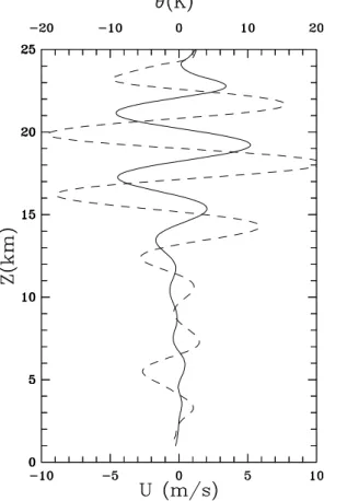
Figure 1a shows vertical profiles of potential temperature and eastward wind com-ponent obtained by the AFRL radiosonde launched on 1 April 2006, 10:05 UTC from the Three Rivers site during T-REX IOP 8. The sonde crossed the Sierra Nevada 20

during its ascent while drifting to the north-east. By the time the sonde reached the lower-stratospheric levels, it was located over the Owens Valley target region (Fig. 3d). Strong mountain wave activity is evident in these profiles, with a large amplitude wave in the lower stratosphere with a dominant vertical wavelength between 3 and 4 km as seen by the radiosonde along its slanted path. Figure 2 shows the fluctuations of po-25

(7)

ACPD

11, 4487–4532, 2011

A. Mahalov et al.

Title Page

Tables Figures

◭ ◮

Back Close

Full Screen / Esc

Discussion

P

a

per

|

Dis

cussion

P

a

per

|

Discussion

P

a

per

|

Discussio

n

P

a

per

phenomenon (Hamming, 1983). The potential temperature and the wind perturbations have large amplitudes and are in quadrature of phase. Based on the polarization rela-tions for gravity waves, which are given by−iωˆθ_¯′

θ =

N2k gmu

′

(Fritts and Alexander, 2003), the latter suggests that these perturbations are gravity waves. We will show in Sect. 4 that these waves are generated by mountains. The apparent vertical wavelength from 5

the radiosonde profile is around 3.8 km. This wavelength reflects both the vertical and horizontal variations in the wave field. As the balloon follows a slanted path through mountain waves with phases lines that are tilted upstream, the radiosonde encounters two equivalent phase surfaces after a vertical displacement that is less than the ac-tual vertical wavelength of the mountain wave (Teitelbaum et al., 1996; Wang et al., 10

2009). Assuming the waves are hydrostatic, i.e. that the horizontal wavelength is much larger than the vertical wavelength, the latter can be estimated fromλ_z=₂_{π U/N}_{. The}

mean wind and stability (U andN) are estimated from the profiles shown in Fig. 1 after smoothing out all fluctuations with wavelengths shorter than 10 km, and averaging the resulting profiles ofU and N between 15 km and 22 km in height. This gives a ver-15

tical wavelength of 4.5 km, which is comparable to the wavelength obtained from the simulation results discussed in Sect. 4.

Similar structures in the stratosphere are also evident in the sounding that was launched from Owens Valley, on the downstream side of the Sierra Nevada on 1 April, 08:00 UTC (Fig. 1b). The downstream sounding features a sharper definition 20

of tropopause around 11 km MSL due to mountain-wave-induced changes to stability. In addition, these profiles reveal pronounced perturbations at low- to mid-tropospheric levels such as a wind reversal near the ground with negative values around−5 m s−1 near 1.8 km MSL, and wind increasing above this altitude and reaching approximately 25 m s−1 around 5 km MSL. The potential temperature is well mixed at low levels with 25

(8)

ACPD

11, 4487–4532, 2011

A. Mahalov et al.

Title Page

Tables Figures

◭ ◮

Back Close

Full Screen / Esc

Discussion

P

a

per

|

Dis

cussion

P

a

per

|

Discussion

P

a

per

|

Discussio

n

P

a

per

|

3 Computational method and numerical setup

The simulations presented in this study use WRF and microscale models. The WRF model is run first, and the output from its innermost nest is used as a coarse grid input for the microscale model. The WRF fields are archived with a frequency of 30 min. The output from WRF is then interpolated in time and space, the latter in both 5

the horizontal and vertical directions, to provide initial and boundary conditions for the microscale model run that is carried out separately. The use of the microscale model is motivated by the fact that the version of the WRF model used in this study does not allow vertical grid refinement.

3.1 WRF simulations

10

The Weather Research and Forecasting (WRF) model is a next generation mesoscale NWP model (Skamarock and Klemp, 2008). It is the first fully compressible conservative-form nonhydrostatic atmospheric model suitable for both research and weather prediction applications. All WRF simulations presented in this study use ver-sion WRF3.1 of WRF-ARW. Among the important upgrades included in verver-sion 3 is 15

the implementation of a new scheme to handle gravity wave reflections near the top of the domain (Klemp et al., 2008). The new technique, based on implicit absorbing layer placed near the top of the domain, is eff_{ective and robust.}

The WRF simulations were performed with three nested domains using two-way nesting. The three WRF domains have the horizontal grid spacing of 27, 9 and 3 km. 20

The number of vertical sigma pressure levels used in all three WRF domains is 61, with a non-uniform distribution in the vertical. The purpose of the non-uniform distri-bution was to achieve an improved resolution near the tropopause and in the lower stratosphere. The pressure at the top is ptop=10 hPa. Numerical simulations were

performed for two events that correspond to IOP 6 and IOP 8 of the T-REX campaign. 25

(9)

ACPD

11, 4487–4532, 2011

A. Mahalov et al.

Title Page

Tables Figures

◭ ◮

Back Close

Full Screen / Esc

Discussion

P

a

per

|

Dis

cussion

P

a

per

|

Discussion

P

a

per

|

Discussio

n

P

a

per

For T-REX IOP 8 case, the WRF simulations were conducted for the period from 31 March, 00:00 UTC to 2 April 2006, 00:00 UTC . Figures 3a–c show the three WRF domains used for this case study. The domains are centered at (36.49◦N, 118.8◦W). Also shown in Figs. 3a–c are the topography and the simulated wind field on 1 April 2006, 08:00 UTC atz=_{12 km. The winds are predominantly south-westerly over the}

5

Sierra Nevada. The thick black curves in Fig. 3 represent the trajectories of two IOP 8 radiosondes from Fig. 1. The black ellipsoidal curve indicates the racetrack pattern of the NSF/NCAR G-V research aircraft in IOP 6.

The WRF simulations were initialized with the high-resolution data provided by the European Centre for Medium-Range Weather Forecasts (ECMWF) global spectral 10

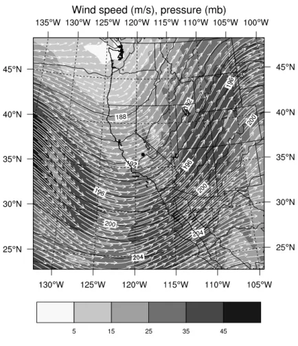
model T799L91. This model has a very high resolution with a spectral triangular trun-cation at horizontal wave number 799, corresponding approximately to a grid spacing of 25 km in the horizontal, and 91 vertical levels up to 0.01 hPa (80 km altitude). Fig-ure 4 shows the synoptic-scale conditions near the T-REX target area on 1 April 2006 during T-REX IOP 8 from the parent WRF domain. Strong southwesterly winds as-15

sociated with a deformed jet are nearly perpendicular to the orientation of the Sierra Nevada creating conditions favorable for mountain wave generation and strong wave dynamics in the stratosphere (Grubiˇsi´c and Billings, 2008).

For the IOP 6 case study, the WRF simulation was conducted for the period from 24 March 2006, 12:00 UTC to 26 March 2006, 12:00 UTC using the same domains as 20

in the IOP 8 case. The synoptic-scale conditions during T-REX IOP 6 were similar to those described above for IOP 8.

3.2 Microscale model

The microscale code used in this study solves the 3-D, fully-compressible, non-hydrostatic equations for atmospheric dynamics. To ensure consistency with WRF, 25

these equations are cast in conservative form and are formulated using a terrain-following pressure coordinate (Laprise, 1992) denoted by η and defined as: η=

(10)

ACPD

11, 4487–4532, 2011

A. Mahalov et al.

Title Page

Tables Figures

◭ ◮

Back Close

Full Screen / Esc

Discussion

P

a

per

|

Dis

cussion

P

a

per

|

Discussion

P

a

per

|

Discussio

n

P

a

per

|

column andpdh,pdht andpdhs represent, respectively, the hydrostatic pressure of the

dry atmosphere, and the hydrostatic pressure at the top and bottom of the dry atmo-sphere. The formulated moist equations are:

∂tU+(∇ ·Vu)η+(α/αd)(αd∂xp+∂ηp∂xφ)=FU (1)

∂tV +(∇ ·Vv)η+(α/αd)(αd∂yp+∂ηp∂yφ)=FV (2) 5

∂tW +(∇ ·Vw)η−g[(α/αd)∂ηp−µd]=FW (3)

∂_tΘ +_{(∇ ·}_V_θ₎

η=Fθ (4)

∂_tµ_d+₍∇ ·V)_η=₀ ₍₅₎

∂tφ+µ−_d1[(V· ∇φ)η−gW]=0 (6)

∂tQm+(∇ ·Vqm)η=FQm (7) 10

In these equations v(u,v,w) is the physical velocity vector, θ is the potential tem-perature, p is the pressure, g is the acceleration of gravity, φ=_gz _{is the}

geopoten-tial, (U,V,W,Ω_,Θ₎=_µ

d(u,v,w,ω,θ), where ω=d η/d t is the vertical velocity in the computational space, and V=₍_U,V,Ω_{) is the coupled velocity vector. The}

right-hand-side terms F_U, F_V, F_W, and F_θ represent forcing terms arising from model physics, 15

subgrid-scale mixing, spherical projections, and the earth’s rotation. The microphysics parametrization uses the Thompson scheme (Thompson et al., 2004). The eddy vis-cosities used for subgrid-scale mixing are computed from the prognostic turbulent ki-netic energy (TKE) equation. The prognostic TKE equations is integrated, including terms for advection, heat flux sources, Reynolds stress sources, diff_{usion and}

dissipa-20

tion (Lilly, 1966). The eddy mixing coeffi_cient_K

m is the related to the turbulence kinetic energy (e) through the expression:K_m=_C

kl e

0.5

(11)

ACPD

11, 4487–4532, 2011

A. Mahalov et al.

Title Page

Tables Figures

◭ ◮

Back Close

Full Screen / Esc

Discussion

P

a

per

|

Dis

cussion

P

a

per

|

Discussion

P

a

per

|

Discussio

n

P

a

per

∂ηφ=−αd (8)

and the diagnostic relation for the full pressure (vapor plus dry air) p =

p0(RdΘm/p0αd)γ. In these equations, αd is the coupled inverse density of the dry air (αd =µd/ρd) and α is the coupled inverse density taking into account the full parcel density α=_α

d(1+qv+qc+qr+qi +...) −1

where q_⋆ are the mixing ra-5

tios (mass per mass of dry air) for water vapor, cloud, rain, ice, etc. Additionally,

Θ

m= Θ(1+(Rv/Rd)qv)≈Θ(1+1.61qv), andQm=µdqm;qm=qv,qc,qi,....

The details of the microscale code and the implicit relaxation used for the bound-ary conditions are described in Mahalov and Moustaoui, 2009. The implicit relaxation boundary scheme consists of progressively constraining the main prognostic variables 10

of the limited area model to match the corresponding values from the coarse grid model in a 9-point large relaxation zone next to the boundary. The microscale nest uses 259 ×241 grid points in the horizontal (1 km grid spacing) and 181 vertical levels up to 10 hPa. Figure 3d shows the topography and the simulated wind at 12 km altitude within the microscale domain on 1 April 2006, 08:00 UTC. As in the WRF simulation, 15

the wind directions are predominantly SW. We note a very smooth relaxation of the wind field at the boundaries of the microscale domain.

4 Simulation results and comparison with observations for T-REX IOP 8

4.1 Comparison between simulations and observations

The comparison between the vertical profiles of potential temperature and the east-20

(12)

ACPD

11, 4487–4532, 2011

A. Mahalov et al.

Title Page

Tables Figures

◭ ◮

Back Close

Full Screen / Esc

Discussion

P

a

per

|

Dis

cussion

P

a

per

|

Discussion

P

a

per

|

Discussio

n

P

a

per

|

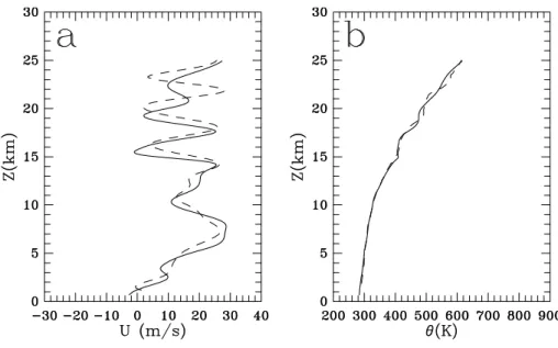
The simulated profiles are interpolated in time and space to the slanted path of the radiosonde. The measured and simulated soundings are fairly close except for some phase errors. Evidently, the microscale model is able to reproduce the fine vertical structure and amplitude of the horizontal wind variation observed by the radiosonde. We note that the apparent vertical wavelength of 3.8 km, reproduced by the microscale 5

model, is smaller than the actual vertical wavelength (4.5 km) and reflects both the ver-tical and horizontal variations along the slanted path of the balloon. Both the potential temperature and wind speed profiles show the well-developed waves and nearly adia-batic layers collocated at the same altitudes (e.g.,z=_{16 km). Another comparison of}

the observed and simulated soundings from IOP 8 is provided in Fig. 6; this one for the 10

sonde launched from Owens Valley on 1 April 2006, 08:00 UTC (cf. Fig. 1b). As with the profile in Fig. 5a, the observed wind profile was filtered to remove small-scale fluc-tuations. In both of these cases the potential temperature profile shows an inversion layer around 5 km and high stability at the tropopause. The observed and simulated profiles are in good agreement.

15

4.2 Simulation results

Figure 7a–d show longitude-altitude cross sections of potential temperature and east-ward wind component on 1 April 2006, 08:00 UTC from the three WRF domains and the microscale nest. These vertical cross-sections show clear evidence of mountain waves, with high activity primarily occurring on the downstream side of the Sierra 20

Nevada. The phase lines of potential temperature exhibit upstream tilt with height that is typical of mountain waves. Comparison of the WRF solutions at diff_{erent horizontal}

resolutions shows a progressive increase in detail in the simulated potential temper-ature and velocity fields with increasing horizontal resolution (Fig. 7a–c). Comparing the solutions from the finest WRF mesoscale nest to that obtained by the microscale 25

(13)

ACPD

11, 4487–4532, 2011

A. Mahalov et al.

Title Page

Tables Figures

◭ ◮

Back Close

Full Screen / Esc

Discussion

P

a

per

|

Dis

cussion

P

a

per

|

Discussion

P

a

per

|

Discussio

n

P

a

per

In addition to improvements in the resolution of fine-scale structures of potential tem-perature and velocity in the UTLS region, noticeable diff_{erences are also evident in the}

flow structure at low levels over Owens Valley, where the microscale model results show a well developed trapped lee wave (Fig. 7d). The trapped lee wave is charac-terized by vertical phase lines (betweenx=_{40 km and} _x=_{60 km in Fig. 7d), and its}

5

amplitude is particularly pronounced around the inversion layer near 5 km, which is also evident in the valley soundings (cf. Fig. 1b). The east-west component of wind shows negative values near the ground (easterly wind), as well as strong shear and positive (westerly) wind near the inversion layer. This clockwise circulation, together with a nearly uniform well-mixed potential temperature field within the valley are indica-10

tive of the presence of a rotor (Grubiˇsi´c and Billings, 2007). An overall similar structure is evident in the finest WRF nest result (Fig. 7c); however, the fine-scale detail within the rotor region is not well resolved and the inversion layer around 5 km is not well developed over the valley.

Figure 8a–b show vertical cross sections of potential temperature and horizontal 15

wind speed across and along Owens Valley on 1 April 2006, 08:00 UTC. The hori-zontal wind speed shown in these figures is the velocity component transverse to the NNW-SSE-oriented valley axis. The cross-valley vertical sections show flow field due to trapped lee waves in the lower troposphere downwind of the Sierra Nevada, and a vertically propagating mountain wave with vertical wavelength around 4.5 km in UTLS 20

above Owens Valley (Fig. 8a). The alternate layers of high and low stability in the stratosphere, with two low stability pockets around 13 km and 18 km MSL, are induced by the vertically propagating mountain wave. The attendant wind field variations fol-low the same pattern with weak winds in the fol-low stability regions and strong winds in the high stability zones. These relationships are similar to those observed in the 25

radiosonde profiles in Fig. 1a.

(14)

ACPD

11, 4487–4532, 2011

A. Mahalov et al.

Title Page

Tables Figures

◭ ◮

Back Close

Full Screen / Esc

Discussion

P

a

per

|

Dis

cussion

P

a

per

|

Discussion

P

a

per

|

Discussio

n

P

a

per

|

field, in between two zones of strong cross-valley flow reaching close to the valley floor (Fig. 8b). This along-valley variation of the flow appears to be related to the lee-side terrain of the Sierra Nevada and the attendant position of the leading edge of the lee wave and rotor. Where the along-valley cross section cuts closer to the high terrain (0< x <20 km in Fig. 8b) we find evidence of downslope winds in a lee-wave trough: 5

a shallow stably-stratified layer of strong winds reaching down to the ground, topped by weaker stratification and weaker winds aloft. In the middle portion of this vertical cross-section, where the Sierra Nevada terrain curves slightly away from line IV in Fig. 3d (30< x <70 km in Fig. 8b), the vertical cross section cuts through the lee wave close to its crest and the rotor zone underneath: the flow near the ground is weak, 10

in places even reversed, and potential temperature well mixed; on top of this there is a pronounced inversion and strong flow in the troposphere above 5 km MSL. In the stratosphere, where the flow is dominated by the vertically propagating mountain wave, there is less variation of the flow structure in the along-valley direction; nevertheless, small-scale three-dimensional variation of the flow is evident there as well (Fig. 8b). 15

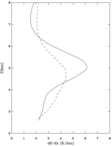
In Fig. 8c-d the same cross-sections are shown at 06:00 UTC. While the overall struc-ture of the flow at these two times is similar, a closer inspection reveals diff_{erences both}

at the lower tropospheric levels as well as in the UTLS region. At 06:00 UTC, the in-version around 5 km MSL is not nearly as well developed as it is at 08:00 UTC. The concentration of the lower-tropospheric stability near the inversion is even more evi-20

dent in Fig. 9, in which profiles of vertical gradients of potential temperature at lower levels above Owens Valley (36.78◦N, 118.28◦W) are compared at the two times.

In the UTLS region above Owens Valley (20< x <40 km in Fig. 8c), we note the presence of secondary wave-like fluctuations that are collocated with strong vertical shear of the horizontal wind. The wind shear owes its origin to the primary mountain 25

(15)

ACPD

11, 4487–4532, 2011

A. Mahalov et al.

Title Page

Tables Figures

◭ ◮

Back Close

Full Screen / Esc

Discussion

P

a

per

|

Dis

cussion

P

a

per

|

Discussion

P

a

per

|

Discussio

n

P

a

per

is more evident in Fig. 10a, which provides a zoom view of potential temperature and vertical velocity in this region. The perturbations are reflected in the vertical velocity field as well, giving rise to strong updrafts and downdrafts reaching up to±5–7ms−1. The horizontal wavelength of these small-scale perturbations is close to 7 km – too short to be directly excited by topography. Furthermore, there is not much evidence 5

for such short waves at upper tropospheric levels below 10 km. In the next section, we examine the properties and generation mechanisms of these small-scale perturbations in more detail.

5 Characteristics and generation mechanism of short fluctuations in UTLS

during IOP 8

10

In this section we examine in more detail the characteristics and generation mechanism of short fluctuations in UTLS illustrated in Figs. 8 and 10 described in Sect. 4. As noted earlier, these fluctuations form in regions of high vertical wind shear due to the primary mountain wave. Before focusing on the physical properties of these short-wavelike fluctuations we note that the vertical grid refinement appears critical for resolving these 15

fine-scale features. In Fig. 10b the same zoomed cross section is shown as in Fig. 10a but with results from the microscale simulation in which the grid refinement was applied in the horizontal direction only. The absence of the fine-scale features in Fig. 10b (no vertical grid refinement) is striking. This shows that the vertical grid refinement is critical for resolving small-scale structures and for numerically simulating dynamical processes 20

in UTLS that lead to their generation.

5.1 Characteristics of short fluctuations

Figure 11 shows co-spectra of the eastward wind component and vertical velocity simu-lated by the microscale model. These co-spectra were calcusimu-lated at each vertical level along a horizontal segment ofL=_{100 km in length over the valley (a portion of dashed}

(16)

ACPD

11, 4487–4532, 2011

A. Mahalov et al.

Title Page

Tables Figures

◭ ◮

Back Close

Full Screen / Esc

Discussion

P

a

per

|

Dis

cussion

P

a

per

|

Discussion

P

a

per

|

Discussio

n

P

a

per

|

line II in Fig. 3d). The two curves in Fig. 11 show vertically averaged co-spectra within UTLS (10 km< z <14 km) and at mid- and upper-tropospheric levels (6< z <10 km). The mountain wave dominates the spectra in both regions. The co-spectra show a peak at horizontal wavenumberkL/2π=_{2, which corresponds to the horizontal wavelength}

of λ≈50 km. Around this wavelength the co-spectra are negative. Negative values 5

of the horizontal and vertical velocity co-spectra are expected for upward propagating mountains waves in the westerly mean flow. The UTLS co-spectrum shows another peak at shorter wavelengths around λ≈7.4 km, which corresponds to wavenumber

kL/2π=₁₃_._{5. This peak is positive indicating a reversal in sign of the co-spectrum.}

The short-wavelength co-spectrum peak is not present at lower levels; this confirms 10

that these short-wavelike fluctuations do not originate at mid- and upper-tropospheric levels.

Based on these co-spectra, the model fields were filtered at each level to remove the primary mountain wave. The band pass filter spans a range of wavelengths between 5 and 12 km. The filtered fields are then used to calculate the local distribution of mo-15

mentum flux associated with the short-wavelike fluctuations. This spatial distribution is obtained by locally averaging the momentum flux within a running window of 24 km in width. Figure 12 shows the vertical cross section of momentum flux associated with the wavelike fluctuations. The positive momentum flux associated with the short-wavelike fluctuations is confined betweenz=_{11 km and}_z=_{13 km in the UTLS region}

20

(Fig. 12). No wave-like activity of this type is found belowz=_{10 km. In the horizontal,}

these fluctuations are found above Owens Valley only (40 km< x <60 km). The verti-cal profile of momentum flux averaged over the valley (Fig. 13) is positive with strong divergence near z=_{12 km – the level at which the primary mountain wave induces}

high vertical shear of the horizontal wind (Fig. 8c). The vertical profile of heat flux, also 25

(17)

ACPD

11, 4487–4532, 2011

A. Mahalov et al.

Title Page

Tables Figures

◭ ◮

Back Close

Full Screen / Esc

Discussion

P

a

per

|

Dis

cussion

P

a

per

|

Discussion

P

a

per

|

Discussio

n

P

a

per

fluxes associated with these short fluctuations are such that the flux divergences tend to mix the potential temperature and to reduce the shear induced by the primary wave (∂u/∂t=₋₁_/ρ_×_∂₍_ρu′_w′₎_/∂z_,_∂θ/∂t₌₋₁_/ρ_×_∂₍_ρθ′_w′₎_/∂z_).

5.2 Generation mechanism

In order to show that the characteristics of the short-wavelike perturbations in the UTLS 5

described above are associated with shear instability, an idealized simulation was car-ried out using a two-dimensional Boussinesq version of the anelastic spectral model presented in Mahalov et al. (2007). The domain is 100 km wide with periodic boundary conditions in the horizontal, and 15 km deep extending from 5 km to 20 km in altitude. The background potential temperature and horizontal wind profiles used in the ideal-10

ized simulation are shown in Fig. 14a. These profiles are obtained from the IOP 8 microscale model run after locally smoothing out the short-wavelike fluctuations and keeping the primary mountain wave. The Richardson number calculated from these profiles shows that the necessary condition for KHI (Ri≤0.25) is satisfied in the altitude range between 12 and 13 km (Fig. 14b). Consequently, the idealized model simulation 15

is initialized by adding a very small random perturbation to the background tempera-ture profile. Figure 15a shows a vertical cross section of potential temperatempera-ture and vertical velocity from the idealized simulation. The corresponding cross section from the real-data IOP 8 microscale simulations is shown in Fig. 15b. It should be noted that the intent here is not to reproduce the exact structure obtained in the real-data simu-20

lation but to investigate the shear instability as a possible generation mechanism for the short-wavelike fluctuations; the shear layer from the real-data simulation is slightly tilted reflecting the upstream tilt of the mountain wave, whereas the temperature and the wind used in the idealized simulation depend on the altitude only. The horizon-tal wavelength of short-wavelike perturbations in the idealized simulation results is 25

(18)

ACPD

11, 4487–4532, 2011

A. Mahalov et al.

Title Page

Tables Figures

◭ ◮

Back Close

Full Screen / Esc

Discussion

P

a

per

|

Dis

cussion

P

a

per

|

Discussion

P

a

per

|

Discussio

n

P

a

per

|

(Fig. 15a) are similar to those in the real-data simulation (Fig. 15b). Furthermore, the vertical profiles of heat and momentum fluxes obtained from the idealized model run (Fig. 16) show strong divergence near the maximum of the wind shear (z≈12 km) with signs and shapes that are in remarkable agreement with those obtained for the real case simulation (Fig. 13). Since the only mechanism present in the idealized case is 5

the shear instability, we conclude that the short-wavelike fluctuations observed in the UTLS region are due to Kelvin-Helmholtz instability.

6 Distributions of O3, CO, temperature and vertical velocity observed in UTLS

during IOP 6

6.1 Comparison between simulations and observations

10

Further validation of the model is provided by the comparison of aircraft measurements and model-simulated potential temperature, vertical velocity, eastward and northward wind components along a large portion of the NSF/NCAR G-V track during IOP 6 on 25 March 2006 (Figs. 17a–c). The fields simulated by the microscale model have been interpolated in time and space to the path of the aircraft. The selected portion of the 15

aircraft flight is about 5.5 h long and was flown between 12 and 13 km in altitude in the lower stratosphere along the racetrack pattern (cf. Fig. 3d). Pronounced and regu-lar fluctuations – signatures of mountain waves – are evident in all fields. The vertical velocity shows updrafts and downdrafts up to±6 m s−1. A good agreement is found be-tween the measured and model simulated fields, which are shown in the same panels. 20

(19)

ACPD

11, 4487–4532, 2011

A. Mahalov et al.

Title Page

Tables Figures

◭ ◮

Back Close

Full Screen / Esc

Discussion

P

a

per

|

Dis

cussion

P

a

per

|

Discussion

P

a

per

|

Discussio

n

P

a

per

6.2 Impact of vertical velocity and gradients on short fluctuations of O₃and CO

6.2.1 Variations in the amplitudes of O3and CO

Figure 19 compares observed variations of vertical velocity (Fig. 19a); and O3, CO

and potential temperature (Fig. 19b) along the same portion of the aircraft flight as in (Fig. 18b). Overall, the amplitudes of the short fluctuations in O₃ and CO follows the 5

amplitudes observed in vertical velocity. For example, around times 2.5 h and 2.8 h, the magnitude of vertical velocity is more than 4 m/s, and the amplitudes of the short fluctuations observed in O₃ and CO around these times are also higher compared to those found at other times (i.e. around 2.6 h). The amplitudes of the short fluctuations in O3and CO vary along the path of the flight. They are relatively high between 2.3 h and

10

2.52 h, and between 2.74 h and 2.80 h (note that the amplitude of CO between 2.74– 2.80 h is smaller than that found between 2.30–2.52 h); and are small between times 2.52 h–2.74 h, where the vertical velocity also shows values with small magnitudes. A closer look to Fig. 19a–b reveals, however, that there are flight times where the amplitude of O₃ and CO do not follow those of vertical velocity. For instance, around 15

times 2.38 h and 2.68 h, the magnitude of vertical velocity have comparable values that are between 1 m/s and 2 m/s. On the other hand, the amplitude of the fluctuations found in CO and O₃ at 2.68 h are very small compared to those present at 2.38 h. This suggests that, although the vertical motion induced by waves is responsible for the fluctuations found in the tracers, the variation of the amplitude of vertical motion 20

observed along the flight track does not explain by itself the variation of the amplitudes seen in the fluctuations of tracers.

6.2.2 Variations in the phases of O₃and CO

Comparison between the phases observed in the short fluctuations of O3and potential

temperature (Fig. 19b) reveals that O₃and potential temperature have same phases, 25

(20)

ACPD

11, 4487–4532, 2011

A. Mahalov et al.

Title Page

Tables Figures

◭ ◮

Back Close

Full Screen / Esc

Discussion

P

a

per

|

Dis

cussion

P

a

per

|

Discussion

P

a

per

|

Discussio

n

P

a

per

|

the relationship between these phases changes sign, and the correlation between O₃ and potential temperature becomes negative. On the average, the phase relationship between the short fluctuations of CO and potential temperature shows negative corre-lation with higher amplitudes for times less than 2.52 h. The correcorre-lations are not well defined beyond 2.52 h because the amplitude of CO is much smaller.

5

6.2.3 The role of the vertical gradients

As shown above the vertical motion does not explain by itself the changes in ampli-tudes and phases of O₃ and CO. Previous studies have shown that the fluctuations of tracers produced by the vertical motion in the presence of gravity waves depends on the vertical mean gradients of tracers (Moustaoui et al., 2010; Teitelbaum et al., 10

1996; Moustaoui et al., 1999). We therefore expect the mean gradients of O₃ and CO to change in magnitude along the portion of the flight presented in Figs. 19a–b. The mean gradient of O3 is also expected to change sign along the same portion in order

to account for the reversal of phases and correlations between O₃ and potential tem-perature. Figure 20 shows the mean vertical profiles of O3 and CO derived from the

15

aircraft measurements. The way these profiles were calculated is described in detail in Moustaoui et al. (2010). Here we give a brief explanation. The mean profiles of O₃and CO are obtained by collecting each individual value of ozone, CO and potential tem-perature from the observations during the entire flight. Then for each value of potential temperature, the collected values of O3and CO are averaged. The resulting O3 and

20

CO profiles are then smoothed using a running mean to obtain the mean O₃and CO profiles presented in Fig. 20.

The mean O3have a positive gradient between 330 K and 342 K, and negative

gra-dient within a layer between 342 K and 356 K. The mean gragra-dient of CO shows high negative value below 342 K, and small values above 342 K. Looking back to Fig. 19b, 25

(21)

ACPD

11, 4487–4532, 2011

A. Mahalov et al.

Title Page

Tables Figures

◭ ◮

Back Close

Full Screen / Esc

Discussion

P

a

per

|

Dis

cussion

P

a

per

|

Discussion

P

a

per

|

Discussio

n

P

a

per

expected to produce fluctuations of O₃ (CO) with relatively high amplitudes that are positively (negatively) correlated with potential temperature. This explains the behavior observed in the fluctuations of O3and CO for times between 2.30 and 2.52 (Fig. 19b).

On the other hand, beyond flight times of 2.52h, the potential temperature is on the average between 340 K and 350 K where the mean gradient of O3 is negative, and

5

where that of CO is small (Fig. 20). The waves evolving in these gradients will then produce fluctuations with negative correlations for O₃ and small amplitudes for CO. This behavior is also clearly seen in O3and CO fluctuations. Thus our explanation for

the variations of amplitudes and phases, and the role of the vertical motion and the mean gradients is supported by the observations.

10

To further confirm the above explanation, the variations of O₃ and CO are recon-structed from those of potential temperature shown in Fig. 19b and from the smoothed mean profiles of these tracers presented in Fig. 20. For each observed value of poten-tial temperature along the portion of the flight, we calculate O₃and CO corresponding to that value from the mean profiles (Fig. 20). The resulting reconstructed fluctuations 15

of CO and O3 are presented in Fig. 19c. These profiles are in good agreement with

those observed along the aircraft path (Fig. 19b). The observed changes in ampli-tudes and phases of O3 and CO are very well reproduced. The correlations between

reconstructed and the observed variations are 0.91 for O3, and 0.91 for CO. Thus, the

reconstructed variations support our explanation of the behavior of the fluctuations ob-20

served in O3 and CO, and confirm the role of both the vertical motion and the mean

gradients on the distributions of these tracers.

7 Conclusions

In this paper we presented results of high-resolution simulations of mountain waves un-der real atmospheric conditions documented during two Intense Observational Periods 25

(22)

ACPD

11, 4487–4532, 2011

A. Mahalov et al.

Title Page

Tables Figures

◭ ◮

Back Close

Full Screen / Esc

Discussion

P

a

per

|

Dis

cussion

P

a

per

|

Discussion

P

a

per

|

Discussio

n

P

a

per

|

Refined vertical gridding has been developed and applied within a microscale model that is driven by data from the finest domain of the WRF model. In the vertical, this refined grid had 181 points with a significantly improved resolution in the UTLS region. This number of grid points in the vertical is significantly higher than the number of vertical levels typically used in NWP models.

5

Comparisons of in situ radiosonde and aircraft observations obtained during the two T-REX IOPs with fields simulated by the microscale model show favorable agreement with comparable wavelengths and amplitudes of perturbations related to the primary mountain wave as well as the secondary short perturbations in the UTLS. For the comparison the model simulated fields were interpolated in space and time to the ra-10

diosonde trajectories as well as to the flight path of the HIAPER aircraft. The degree of agreement between the microscale model simulations and the observations is encour-aging given the diffi_{culty in accurately predicting the exact timing and location of}

small-scale features such as those associated with secondary perturbations in the UTLS and given many uncertainties related to initial conditions, interpolation of simulation results 15

to the positions of measurements, phase lag between the simulated and observed dis-turbances, etc. Despite all these limitations, the comparisons between the simulation results and observations is more than reasonable and provides a solid verification for the microscale model.

We showed that the vertical grid refinement, achieved in this study with the use of 20

the microscale model, is critical for resolving small-scale perturbations in UTLS and for numerically simulating dynamical processes that lead to their generation. Hori-zontal nesting alone was proved to be insuffi_{cient for this purpose. Furthermore, the}

increased vertical resolution aff_{orded by the vertical grid refinement was proved also to}

be beneficial for resolving the inversion layer related to the trapped lee waves at lower 25

(23)

ACPD

11, 4487–4532, 2011

A. Mahalov et al.

Title Page

Tables Figures

◭ ◮

Back Close

Full Screen / Esc

Discussion

P

a

per

|

Dis

cussion

P

a

per

|

Discussion

P

a

per

|

Discussio

n

P

a

per

fluctuations in UTLS and the attendant vertical profiles of heat and momentum fluxes show that they are generated by Kelvin-Helmholtz instability along shear lines locally induced by the primary mountain wave. The idealized numerical simulation carried out using real temperature and wind profiles obtained from the microscale simulation con-firmed that the short perturbations, despite visual resemblance, are not trapped gravity 5

waves but instead small-scale wave motions resulting from Kelvin-Helmholz instability. We also showed that the variations found in the magnitude of vertical velocity do not explain alone those observed in the amplitudes of O3and CO, even though the latter

are produced by the vertical motion induced by mountain waves. We showed that the combination of both the vertical motion and the local vertical gradients of O₃ and CO 10

account for the modulations of amplitudes and phases found in the variations of these tracers.

Finally, while the grid refinement provided by the microscale model in this study al-lowed resolution of certain scales of shear instability, the full dynamics of perturbations at these scales remains constrained by the allowable resolution and the subgrid-scale 15

parametrization. Much higher resolution, in both the horizontal and vertical directions, is needed to fully resolve fine turbulence scales associated with shear instability.

Acknowledgements. This work is sponsored in part by AFOSR contract FA9550-08-1-0055 and by the NSF CMG grant 0934592 to the Arizona State University; and NSF grant ATM-0524891 to the Desert Research Institute which provided support to VG in early stages of this 20

work. We thank the WRF group at NCAR for providing the WRF code.The outstanding eff_orts of the T-REX field campaign participants and the T-REX staff_{are greatly appreciated. We are} thankful to T. L. Campos for CO data and I. B. Pollack for O₃data.

References

Alexander, M. J. and Teitelbaum, H.: Observation and analysis of a large amplitude 25

(24)

ACPD

11, 4487–4532, 2011

A. Mahalov et al.

Title Page

Tables Figures

◭ ◮

Back Close

Full Screen / Esc

Discussion

P

a

per

|

Dis

cussion

P

a

per

|

Discussion

P

a

per

|

Discussio

n

P

a

per

|

Bacmeister, J. T. and Schoeberl, M. R.: Breakdown of vertically propagating two-dimensional gravity waves forced by orography, J. Atmos. Sci., 46, 2109–2134, 1989.

Danielsen, E. F., Hipskind, R. S. Starr, W. L. Vedder, J. F. Gaines, S. E., Kley, D., and Kelly K. K.: Irreversible transport in the stratosphere by internal waves of short vertical wavelength, J. Geophys. Res., 96, 17433–17452, 1991.

5

Dornbrack, A.: Turbulent mixing by breaking gravity waves, J. Fluid Mech., 375, 113–141, 1998.

Dornbrack, A., Birner, T., Fix, A., Flentje, H., Meister, A., Schmid, H., Bromwell, E., and Ma-honey, M.: Evidence for intertia gravity waves forming polar stratospheric clouds over Scan-dinavia, J. Geophys. Res., 107, 8287, doi:10.1029/2001JD000452, 2002.

10

Doyle, J., Shapiro, M., Jiang, Q., and Bartels, D.: Large-amplitude mountain wave breaking over Greenland, J. Atmos. Sci., 62, 3106-3126, 2005.

Grubiˇsi´c, V and Billings, B. J.: The intense lee-wave rotor event of Sierra Rotors IOP 8, J. Atmos. Sci., 64, 4178–4201, 2007.

Grubiˇsi´c, V. and Billings, B. J.: Climatology of the Sierra Nevada mountain-wave events, Mon. 15

Wea. Rev., 136, 757–768, 2008.

Grubiˇsi´c, V., Doyle, J. D., Kuettner, J., Mobbs, S., Smith, R. B., Whitman, D., Dirks, R., Czyzyk, S., Cohn, S. A, Vosper, S., Weissmann, M., Haimov, S., De Wekker, S. J. F., Pan, L. L., and Chow, F. K.: The Terrain-induced Rotor Experiment: A field campaign overview with some highlights of special observations, Bull. Amer. Meteor. Soc., 89, 1513–1533, 2008.

20

Hamming, R. W.: Digital filters, Englewood Cliff_{s, N. J.: Prentice-Hall, 1983.}

Joseph, B., Mahalov, A., Nicolaenko, B. and Tse, K. L.: Variability of turbulence and its outer scales in a nonuniformly stratified tropopause jet, J. Atmos. Sci., 41, 524–537, 2004. Kirkwood, S., Mihalikova, M., Rao, T. N., and Satheesan, K.: Turbulence associated with

moun-tain waves over Northern Scandinavia a case study using the ESRAD VHF radar and the 25

WRF mesoscale model, Atmos. Chem. Phys., 10, 3583–3599, doi:10.5194/acp-10-3583-2010, 2010.

Klemp, J. B., Dudhia J., and Hassiotis, A.: An upper gravity wave absorbing layer for NWP applications, Mon. Wea. Rev., 136, 3987–4004, 2008.

Lane, T. P. and Sharman, R. D.: Gravity wave breaking, secondary wave generation, and mixing 30

above deep convection in a three-dimensional cloud model, Geophys. Res. Lett., 33, L23813, doi:10.1029/2006GL027988, 2006.

(25)

vari-ACPD

11, 4487–4532, 2011

A. Mahalov et al.

Title Page

Tables Figures

◭ ◮

Back Close

Full Screen / Esc

Discussion

P

a

per

|

Dis

cussion

P

a

per

|

Discussion

P

a

per

|

Discussio

n

P

a

per

able, Mon. Wea. Rev., 120, 197–207, 1992.

Lott, F., and Teitelbaum, H.: Nonlinear dissipative critical level interaction in a stratified shear flow: instabilities and gravity waves, Geophys. Astro. Fluid., 66, 133–167, 1992.

Lilly, D. K.: On the instability of Ekman boundary flow, J. Atmos. Sci., 23, 481–494, 1966. Mahalov, A. and Moustaoui, M.: Vertically nested non-hydrostatic model for multi-scale reso-5

lution of flows in the Upper Troposphere and Lower Stratosphere, J. Comp. Physiol., 228, 1294–1311, 2009.

Mahalov, A. and Moustaoui, M.: Characterization of atmospheric optical turbulence for laser propagation, Laser Photonics. Rev., 4, 144–159, doi:10.1002/lpor.200910002, 2010.

Mahalov, A., Moustaoui, M., Nicolaenko, B., and Tse, K. L.: Computational studies of inertia-10

gravity waves radiated from upper tropospheric jets, Theor. Comput. Fluid. Dyn., 21, 399– 422, 2007.

Mahalov, A., Moustaoui, M., and Nicolaenko, B.: 3-D Instabilities in shear stratified non-parallel flows, Kinetic and Related Models, 2, 215–229, 2009.

Moustaoui, M., Teitelbaum, H., Van Velthoven, P. F. J., and Kelder, H.: Analysis of gravity waves 15

during the POLINAT experiment and some consequences for stratosphere-troposphere ex-change, J. Atmos. Sci., 56, 1019–1030, 1999.

Moustaoui, M., Joseph, B., and Teitelbaum, H.: Mixing layer formation near the tropopause due to gravity wave-critical level interactions in a cloud-resolving model, J. Atmos. Sci., 61, 3112–3124, 2004.

20

Moustaoui, M., Mahalov, A., Teitelbaum, H. and Grubiˇsic’, V.: Nonlinear modulation of O₃ and CO induced by mountain waves in the upper troposphere and lower stratosphere during terrain-induced rotor experiment, J. Geophys. Res., 115, D19103, doi:10.1029/2009JD013789, 2010.

Pluogonven, R., Hertzog, A., and Teitelbaum, H.: Observations and simulations of a large-25

amplitude mountain wave breaking over the Antarctic Peninsula, J. Geophys. Res., 113, D16113, doi:10.1029/2007JD009739, 2008.

Prusa, J. M., Smolarkiewicz, P. K., and Garcia, R. R.: Propagation and breaking at high altitudes of gravity waves excited by tropospheric forcing, J. Atmos. Sci., 53, 2186–2216, 1996. Satomura, T. and Sato, K.: Secondary generation of gravity waves associated with the breaking 30

of mountain waves, J. Atmos. Sci., 56, 3847–3858, 1999.

(26)

ACPD

11, 4487–4532, 2011

A. Mahalov et al.

Title Page

Tables Figures

◭ ◮

Back Close

Full Screen / Esc

Discussion

P

a

per

|

Dis

cussion

P

a

per

|

Discussion

P

a

per

|

Discussio

n

P

a

per

|

investigations and modelling studies, Ann. Geophys., 24, 2863-2875, 2006, http://www.ann-geophys.net/24/2863/2006/.

Skamarock, W. C. and Klemp, J. B.: A time-split nonhydrostatic atmospheric model for weather research and forecasting applications, J. Comp. Physiol., 227, 3465–3485, 2008.

Smith, R. B., Woods, B. K., Jensen, J., Cooper, W. A., Doyle, J. D., Jiang, Q., and Grubiˇsi´c, V.: 5

Mountain waves entering the stratosphere, J. Atmos. Sci., 65, 2543–2562, 2008

Teitelbaum, H., Moustaoui, M., Ovarlez, J., and Kelder, H.: The role of atmospheric waves in the laminated structure of ozone profiles at high latitude, Tellus, 48A, 442–455, 1996. Teitelbaum, H., Moustaoui, M., Sadourny, R., and Lott, F.: Critical levels and mixing layers

induced by convectively generated gravity waves during CEPEX, Quart. J. Roy. Meteor. Soc., 10

125, 1715–1734, 1999.

Thompson, G., Rasmussen, R. M., and Manning, K.: Explicit forecasts of winter precipitation using an improved bulk microphysics scheme. Part 1: Description and sensitivity analysis, Mon. Wea. Rev., 132, 519–542, 2004.

Vosper, S. B. and Worthington, R. M.: VHF radar measurements and model sim-15

ulations of mountain waves over Wales, Q. J. Roy. Meteor. Soc., 128, 185-204, doi:10.1256/00359000260498851, 2002.

Wang, P. K.: Moisture plumes above thunderstorm anvils and their contributions to cross-tropopause transport of water vapor in midlatitudes, J. Geophys. Res., 108 , 4194, doi:10.1029/2002JD002581, 2003.

20

Wang J., Bian, J., Brown, W. O. J., Cole, H., Grubiˇsi´c, V. , and Young, K.: Vertical air motion from T-REX radiosonde and dropsonde data, J. Atmos. Tech., 26, 928–942, 2009.

(27)

ACPD

11, 4487–4532, 2011

A. Mahalov et al.

Title Page

Tables Figures

◭ ◮

Back Close

Full Screen / Esc

Discussion

P

a

per

|

Dis

cussion

P

a

per

|

Discussion

P

a

per

|

Discussio

n

P

a

per

(28)

ACPD

11, 4487–4532, 2011

A. Mahalov et al.

Title Page

Tables Figures

◭ ◮

Back Close

Full Screen / Esc

Discussion

P

a

per

|

Dis

cussion

P

a

per

|

Discussion

P

a

per

|

Discussio

n

P

a

per

|

(29)

ACPD

11, 4487–4532, 2011

A. Mahalov et al.

Title Page

Tables Figures

◭ ◮

Back Close

Full Screen / Esc

Discussion

P

a

per

|

Dis

cussion

P

a

per

|

Discussion

P

a

per

|

Discussio

n

P

a

per

(30)

ACPD

11, 4487–4532, 2011

A. Mahalov et al.

Title Page

Tables Figures

◭ ◮

Back Close

Full Screen / Esc

Discussion

P

a

per

|

Dis

cussion

P

a

per

|

Discussion

P

a

per

|

Discussio

n

P

a

per

|

(31)

ACPD

11, 4487–4532, 2011

A. Mahalov et al.

Title Page

Tables Figures

◭ ◮

Back Close

Full Screen / Esc

Discussion

P

a

per

|

Dis

cussion

P

a

per

|

Discussion

P

a

per

|

Discussio

n

P

a

per

(32)

ACPD

11, 4487–4532, 2011

A. Mahalov et al.

Title Page

Tables Figures

◭ ◮

Back Close

Full Screen / Esc

Discussion

P

a

per

|

Dis

cussion

P

a

per

|

Discussion

P

a

per

|

Discussio

n

P

a

per

|

(33)

ACPD

11, 4487–4532, 2011

A. Mahalov et al.

Title Page

Tables Figures

◭ ◮

Back Close

Full Screen / Esc

Discussion

P

a

per

|

Dis

cussion

P

a

per

|

Discussion

P

a

per

|

Discussio

n

P

a

per