ISSN 1549-3644
© 2012 Science Publications
Corresponding Author: Wan Zawiah Wan Zin, School of Mathematical Sciences, Faculty of Science and Technology,
University Kebangsaan Malaysia, 43600 UKM Bangi, Selangor, Malaysia Tel: 03-8921 5790 Fax: 03-8921 3289
Bayesian Changepoint
Analysis of the Extreme Rainfall Events
Wan Zawiah Wan Zin,
Abdul Aziz Jemain and Kamarulzaman Ibrahim
School of Mathematical Sciences, Faculty of Science and Technology
University Kebangsaan Malaysia, 43600 UKM Bangi, Selangor, Malaysia
Abstract: Problem statement: This study assesses recent changes in extremes of annual rainfall in Peninsular Malaysia based on daily rainfall data for 50 rain-gauged stations over the period 1975-2004.
Approach: Eight indices that represent the extreme events are defined and analyzed, which are extreme Dry Spell (XDS), extreme Rain-Sum (XRS), extreme wet-day intensities at 95% and 99% percentiles (I95 and I99), proportion of extreme rainfall amount to the total rainfall amount (R95& R99) and frequency of extreme wet-day at 95 and 99% percentiles (N95 and N99). Bayesian approach based on a single shifting model is used to investigate the change in the mean level of these extreme rainfall indices. The detection on whether the change has occurred or not is analyzed followed by the estimation of the location of change point. Results: The results of the analysis showed that half of the stations considered displayed significant changes. The analysis also found that in general, the changes occurred in the early 90s. More than 75% of the stations which recorded significant changes are situated on the west coast of the peninsula. Conclusion/Recommendations: The west coast of Peninsular Malaysia displays more significant changes in trend especially at stations located in urban areas compared to the east coast of the peninsula. In terms of the Bayesian methods used, the existence of any outlier in the data series may influence the result since the analysis is based on mean value which is very sensitive to any outlier.
Key words: Bayesian method, changepoint, time series, hydrology
INTRODUCTION
The phenomenon of extreme precipitation events, which include extreme rainfall and extremely long spell of dry days (drought), are among the most disruptive of atmospheric phenomena. These events may cause significant damage to agriculture, ecology and infrastructures, disruption towards daily activities, accidents and loss of life. In Peninsular Malaysia, the phenomenon of unpredictable rainfall events which increases in frequency lately has brought about damages costing millions of Malaysian ringgit. The increase in massive flood cases including flash flood and landslides in the recent 10 years is believed to be due to the increase in rainfall intensities. On the other hand, prolonged dry condition has forced the local authorities to impose water rationing, resulting in negative impact to daily life. Apart from that, in agricultural areas, crops can suffer damage from excess rainfall as well as extreme dry spells.
In this context, this research provides an insight to the possible change in the rainfall extreme and extreme dry spell for the past 30 years as measured by 8 extreme
indices. This is because, any changes in extreme rainfall trend brings great implication to engineering, insurance, town planning and any activities that assumed that climate has been stable for the last few decades. For example, the design of drainage, bridge, retaining wall and dam systems depends on the expected rain amount received during certain time duration. Earlier research on the changes in these extreme rainfall indices at the same area using data from only 8 rain-gauged stations can be found from Zin et al. (2010). In their article, the extreme rainfall indices derived from rainfall data at these 8 rain-gauged stations for the period of 35 years have been analysed for any change in trend. The statistical methods used in that study is classical approach where the changes in trend were tested using Mann-Kendall test and linear regression while the change detection points were identified using Pettitt test.
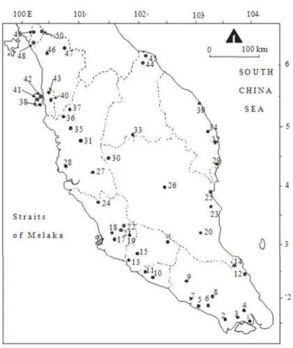
Fig. 1: Location of stations used in this study All the 50 stations, numbered from 1 to 50, are located
at various places throughout Peninsular Malaysia, as shown in Fig. 1. These stations could represent the overall trend for extreme rainfall for the peninsular. We consider the data from 1975 to 2004 because this is the longest period for which a complete set of data is available for all stations. As described Hosking and Wallis (2005), the problem of availability of a large set of data is not uncommon when the analysis is based on the annual series. This situation is common in developing countries where long records are often unavailable; however, studies need to be done for various planning purposes such as for construction of infrastructures.
Peninsular Malaysia experiences a tropical climate due to its location with respect to the equator and the influence of monsoon seasons. It lies in the equatorial zone, situated in the northern latitude between 1°N and 6°N and the eastern longitude from 100°E and 103°E. Throughout the year, the peninsular experiences a wet and humid condition with daily temperature ranges from 25.5-35°C. The two monsoons that contribute to
MATERIALS AND METHODS
Methodology: In this research, the change point analysis focuses on the detection of change in the mean level of the time series data and the location of the change point. Several classical methods in change point analysis include the non-parametric Wilcoxon test, the Student-t test and the sequential Mann-Kendall test. The alternative for these classical approaches is Bayesian approach which takes into consideration prior information, the model of the shift assumed and observed data into forming a posterior distribution to model the associated analysis. The statistical inferences on the unknown parameters with regards to change point location can then be made based on this posterior distribution. Bayesian approach in change identification problem for mean level in time series data have been used by previous researchers such as by Smith (1975), Lee and Heighinian (1977), Booth and Smith (1982), Perreault
et al. (2000a; 2000b) and Kim et al. (2009). The Bayesian approach in this study is based on a single shifting model and takes into consideration non-informative prior distributions on the unknown change point.
In contrast to the classical approach, the Bayesian methods take into consideration the parameters of a model as random variables represented by a statistical distribution (prior distribution) rather than fixed values. The Bayesian methods allow the integration of statistical analysis through the prior distribution with the most current information based on the observations into a posterior distribution. In other words, the prior distribution reflects beliefs about the parameters prior to experimentation; the posterior distribution provides an updated belief about the parameters after sample data is obtained. The analysis involved includes getting the mean values before and after the shift, the amount of change and the variation in observations. In this study, two related problems will be analysed that is on the detection of the change point and the estimation of the change point.
There are several definitions used to describe the extreme precipitation events. In this study, eight extreme indices were examined based on daily rainfall data at 50 stations. Some of the indices chosen are standard extreme precipitation indices as defined by The Expert Team on Climate Change Detection, Monitoring and Indices (ETCCDMI).
The ETCCDMI indices considered in this study are maximum dry spell, maximum cumulative rain-sum, extreme intensities, extreme frequencies and extreme proportions (Table 1). A wet day is defined as a day with a rainfall amount of at least 1 mm. The dry spell index calculates the longest dry spell (rainfall amount less than 1mm) recorded each year. The extreme
rain-sum index measures the greatest cumulative rainfall amount received during a wet spell in a year. This index is considered as flooding usually occurs when infrastructure is unable to accommodate the amount of excess water during prolonged and continuous rainy days. The 95th and 99th percentiles are selected as the thresholds to represent extreme events. Extreme proportion measures the proportion of annual rainfall amount to the total amount of annual rainfall received. Extreme frequency is a count of rainfall events per year which equal to or above the long-term (1975-2004) mean of 95th and 99th percentiles. We will refer to rainfall exceeding 95th percentile as very wet days and exceeding the 99th percentile as extremely wet days.
Consider a set of hydrological time series
{
1 2 n}
X= x , x ,..., x whose due to some exogenous factors, the first and second segments fluctuate, around two different mean levels, denoted by µ1 and µ2 respectively
but with the same variance, σ2
. Assume that the single change point has occurred at time point τ and the time series follow a Normal distribution Eq. 1:
(
2)
i 1
X ~ N µ σ, , i 1,...,= τ
(
2)
i 2
X ~ N µ σ, , i= τ +1,..., n (1)
where
(
2)
kN µ σ, represents a Normal distribution with density function given as Eq. 2:
(
2)
(
k)
2k 2
x 1
f , exp , x
2 2
− µ
µ σ = − ∈
σ
σ π ℝ (2)
The parametersτ, µ1, µ2 and σ 2
represent the change point, the mean before and after the shift and the variance of the series, respectively. The prior distribution of µ1 and µ2 are assumed to be the same
Normal distribution, denoted by Eq. 3 and 4:
(
2)
1~ N 0, 0
µ µ σ (3)
(
2)
2~ N 0, 0
µ µ σ (4)
With large 2 0
σ , these distributions will approach the non-informative prior distributions.
The variance of the series σ2
, is assumed constant and estimated by Eq. 5:
(
)
(
)
n n
2
i i
2 i 1 i 1
x x x
; x
n 1 n
= =
−
σ = =
−
∑
∑
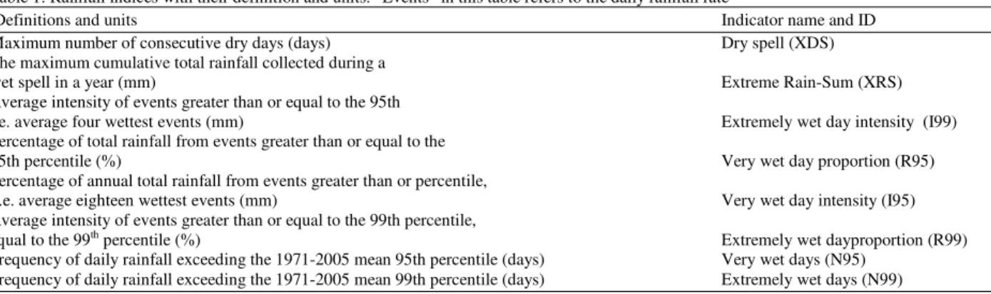
Table 1: Rainfall indices with their definition and units. “Events” in this table refers to the daily rainfall rate
Definitions and units Indicator name and ID
Maximum number of consecutive dry days (days) Dry spell (XDS)
The maximum cumulative total rainfall collected during a
wet spell in a year (mm) Extreme Rain-Sum (XRS)
Average intensity of events greater than or equal to the 95th
i.e. average four wettest events (mm) Extremely wet day intensity (I99)
Percentage of total rainfall from events greater than or equal to the
95th percentile (%) Very wet day proportion (R95)
Percentage of annual total rainfall from events greater than or percentile,
i.e. average eighteen wettest events (mm) Very wet day intensity (I95)
Average intensity of events greater than or equal to the 99th percentile,
equal to the 99th percentile (%) Extremely wet dayproportion (R99)
Frequency of daily rainfall exceeding the 1971-2005 mean 95th percentile (days) Very wet days (N95) Frequency of daily rainfall exceeding the 1971-2005 mean 99th percentile (days) Extremely wet days (N99)
After a sample of time series X is observed, the posterior distribution of the mean levels µ1 and µ1can be
determined using Bayes theorem Eq. 6 and 7:
(
* *2)
(
* *2)
1| X ~ Nτ 1, 1 ; 2| Xτ+1~ N 2, 2
µ µ σ µ µ σ (6)
where:
(
)
(
)
*
0 i 2
* i 1 *2
1 * 1 *
n *
0 i 2
* i 1 *2
2 * 2 *
2 *
2 0
n . x
,
n n
n . x
,
n n n n
n . τ = =τ+ µ + σ
µ = σ =
+ τ + τ
µ +
σ
µ = σ =
+ − τ + − τ
σ =
σ
∑
∑
The likelihood function for τ, µ1 and µ1 can be
derived using this formula,
(
)
(
)
(
)
n
1 2 1 2
i 1 i 1
2 i 1 2 2 i 1 2 n i 2 2 2 i 1
L X | , , f (x ) f (x ) x 1 exp 2 2 x 1 exp 2 2 τ = =τ+ τ = =τ+
τ µ µ =
− µ
= −
σ
πσ
− µ
−
σ
πσ
∏
∏
∏
∏
(7)
Using the Bayes theorem, the posterior distribution of the change point location, τ is Eq. 8:
(
)
(
) ( )
(
) ( )
1 2
1 2 n 1
1 2 j 1
L X | , , .p | X, ,
L X | j, , .p j −
=
τ µ µ τ
π τ µ µ =
µ µ
∑
(8)where p(j) represents the prior distribution of the change point location,τ, assumed to follow a uniform
distribution, that is p j
( ) (
=1 n 1 , j 1,..., n 1.−)
= − Thus Eq. 9:(
)
(
)
(
)
1 2
1 2 n 1
1 2 j 1
L X | , , | X, ,
L X | j, , −
=
τ µ µ π τ µ µ =
µ µ
∑
(9)The justification on whether a shift has occurred or not can be checked using Bayes factor, B Eq. 10:
(
)
(
)
n 1 1 2 j 1 1 2 p 1B . j | X, ,
1 p n | X, ,
−
=
= π τ = µ µ
− π τ = µ µ
∑
(10)p is a constant such that0≤ ≤p 1.
The calculation in this procedure may not be expressed in a simple form but it can be estimated by using Monte Carlo Markov Chain approach.
RESULTS AND DISCUSSION
(a)
(b)
(c)
(d)
(e)
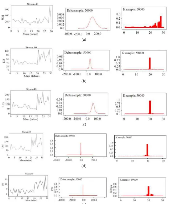
Fig. 2: Time series plot (above) and the posterior probability distribution of the changepoint location (below) for station 40 for extreme indices (a) XRS, (b) I95, (c) I99, (d) N95 dan (e) N99
As an example, the results for station 40, which is one of the two stations with most number of significant changes in extreme indices, are displayed in Fig. 2. For each pair of graphs, the top graph displays the time series plot of the extreme index data while the graph at the bottom of the pair shows the posterior probability plot for change point that is the probability that the change point occurs at a particular point. The largest value represents the point when the shift in trend is most likely to occur.
Table 2: The year when the change point is detected for each station with significant trend. The bold letter refers to significantly increasing trend and the shaded box refers to significantly decreasing trend
Station XDS XRS I95 I99 R95 R99 N95 N99
2 1993 1982 1983
5 1996
6 2003 2003
7 1996
8 2003 2003
11 1997 1978
13 1988 1994
14 1983
16 1984
17 1997 1990 1991
18 1986 1986 1987
20 2002
21 1991
22 1992 1992
26 2002 2002 2002 2002 1999
27 1996 1977
30 1975 1976
32 1976
33 1980
40 1996 1994 1994 1994 1994
43 1995 1996
44 1980
46 1985
47 1990
50 1987 1983
Nevertheless, the existence of data with relatively larger value compared to other data (outlier) may influence the analysis results as this analysis is based on the change in mean value that is rather sensitive towards any outlier in data.
In terms of climatology, the two extreme El-Nino events occurring in 1982/83 and 1997/98 may be the contributing factor to the change in climate as detected by the Bayesian change point detection test. Apart from that, majority of the stations located at the west coast of the peninsula experience significant changes in the studied indices. In general, these areas experience rapid development in late 1980s to early 1990s. This factor may contribute to the obvious climate change compared to the east coast of the peninsula. Shaharuddin (1992; 2004) discovered that there exist effects from Urban Heat Island at big cities which influence the temperature change and directly cause an increase in rainfall intensity at these areas. This can be seen clearly at stations located in Selangor and Federal Territory (stations 17, 18 and 22).
CONCLUSION
As a whole, the west coast of Peninsular Malaysia displays more significant changes in trend compared to the east coast of the peninsula. The increase in significant trend at urban area as seen at station 17, 18 and 22 for extreme cumulative rainfall amount, extreme
intensities and extreme frequency need to be viewed with caution as this area is a highly populated area. Many factors such as rapid township development, industrialisation, increase in the number of vehicles and population may influence the pattern of rainfall for this area where the change in trend is found to begin in the 1980s to early 1990s. Apart from that, climate phenomena such as El-Nino and La-Nina may play important role in determining the weather pattern in Peninsular Malaysia
In terms of the Bayesian methods used, the existence of any outlier in the data series may influence the result since the analysis is based on mean value which is very sensitive to any outlier. This situation may cause the Bayesian change point analysis to show significant change although in fact the other points in that respective station are actually consistent.
ACKNOWLEDGMENT
REFERENCES
Booth, N.B. and A.F.M. Smith, 1982. A Bayesian approach to retrospective identification of change-points. J. Econ. 19: 7-22. DOI: 10.1016/0304-4076(82)90048-3
Hosking, J.R.M. and J.R. Wallis, 2005. Regional Frequency Analysis: An Approach Based on L-Moments. Cambridge University Press, Cambridge, ISBN-10: 0521430453 pp: 224. Kim, C., M.S. Suh and K.O. Hong, 2009. Bayesian
changepoint analysis of the annual maximum of daily and subdaily precipitation over south korea. J.
Climate, 22: 6741-6757. DOI:
10.1175/2009JCLI2800.1
Lee, A.S.F. and S.M. Heghinian, 1977. A shift of the mean level in a sequence of independent normal random variables: A Bayesian approach. Technometrics 19: 503-506. DOI: 10.2307/1267892
Perreault, L., J. Bernier, B. Bobee and E. Parent, 2000a. Bayesian change-point analysis in hydrometeorological time series. Part 1. The normal model revisited. J. Hydrol. 235: 221-241. DOI: 10.1016/S0022-1694(00)00270-5
Perreault, L., J. Bernier, B. Bobee and E. Parent, 2000b. Bayesian change-point analysis in hydrometeorological time series. Part 2. Comparison of change-point models and forecasting. J. Hydrol. 235: 242-263. DOI: 10.1016/S0022-1694(00)00271-7.
Shaharuddin, A., 1992. Some effects of urban parks on air temperature variations in Kuala Lumpur, Malaysia. Proceedings of the 2nd Tohwa University International Symposium on Urban Thermal Environment, Sep. 7-10, Tohwa University, Fukuoka, Japan pp: 107-108.
Shaharuddin, A., 2004. Trends and variability of rainfall in Malaysia: A case of Kuala Lumpur and Kuantan, Pahang. Proceedings of the 3rd Annual Hawaii International Conference on Social Sciences, Jun. 16-19, Waikiki, Hawaii.
Smith, A.F.M., 1975. A Bayesian approach to inference about a change-point in a sequence of random variables. Biometrika 62: 407-416. DOI: 10.1093/biomet/62.2.407