Forecasting accuracy and estimation uncertainty using VAR models with short- and long-term economic restrictions: a Monte-Carlo study

No _{589 ISSN 0104-8910}

Forecasting Accuracy and Estimation

Uncertainty using VAR Models with Short–

and Long–Term Economic Restrictions: A

Monte–Carlo Study

Os artigos publicados são de inteira responsabilidade de seus autores. As opiniões

neles emitidas não exprimem, necessariamente, o ponto de vista da Fundação

Forecasting Accuracy and Estimation Uncertainty using

VAR Models with Short- and Long-Term Economic

Restrictions: A Monte-Carlo Study

Osmani Teixeira de Carvalho Guillén Banco Central do Brasil

Av. Presidente Vargas, 730 - Centro Rio de Janeiro, RJ 20071-001

Brazil João Victor Isslery

Graduate School of Economics – EPGE Getulio Vargas Foundation Praia de Botafogo 190 s. 1111

Rio de Janeiro, RJ 22253-900 Brazil

jissler@fgv.br George Athanasopoulos

Department of Econometrics and Business Statistics Monash University, Clayton, Victoria 3800

Australia

March, 2005.

Abstract

Using vector autoregressive (VAR) models and Monte-Carlo simulation methods we investigate the potential gains for forecasting accuracy and estimation uncertainty of two commonly used restrictions arising from economic relationships. The …rst re-duces parameter space by imposing long-term restrictions on the behavior of economic variables as discussed by the literature on cointegration, and the second reduces pa-rameter space by imposing short-term restrictions as discussed by the literature on

Acknowledgments: Parts os this paper were writen while Osmani T. Guillén and João Victor Issler were visiting Monash University, which hospitality is gratefully acknowledged. João Victor Issler and George Athanasopulos also acknowledge the hospitality of the Australian National University, where parts of this paper were writen. We gratefully acknowledge comments and suggestions given by Alain Hecq, Luiz Renato Lima, and of the participants of the conferencesCommon Features in London andEncontro Brasileiro de Econometria. Special thanks are due to Farshid Vahid for some of the ideas in this paper and his encouragement and support to Osmani T. Guillén during his visit to Monash University and to George Athanasopoulos. The usual disclaimers apply. João Victor Issler and Osmani T. Guillén acknowledge, respectively, the support of CNPq-Brazil, PRONEX, and CAPES fellowship BEX0934/02-0.

serial-correlation common features (SCCF). Our simulations cover three important issues on model building, estimation, and forecasting. First, we examine the per-formance of standard and modi…ed information criteria in choosing lag length for cointegrated VARs with SCCF restrictions. Second, we provide a comparison of fore-casting accuracy of …tted VARs when only cointegration restrictions are imposed and when cointegration and SCCF restrictions are jointly imposed. Third, we propose a new estimation algorithm where short- and long-term restrictions interact to estimate the cointegrating and the cofeature spaces respectively.

We have three basic results. First, ignoring SCCF restrictions has a high cost in terms of model selection, because standard information criteria chooses too frequently inconsistent models, with too small a lag length. Criteria selecting lag and rank simultaneously have a superior performance in this case. Second, this translates into a superior forecasting performance of the restricted VECM over the VECM, with important improvements in forecasting accuracy – reaching more than 100% in extreme cases. Third, the new algorithm proposed here fares very well in terms of parameter estimation, even when we consider the estimation of long-term parameters, opening up the discussion of joint estimation of short- and long-term parameters in VAR models.

Keywords: Reduced rank models, model selection criteria, forecasting accuracy.

JEL Classi…cation: C32, C53.

1

Introduction

One of the objectives of time-series econometrics is to identify relationships between eco-nomic variables and then use them for estimation and forecasting. In theory, an identi…ed relationship should improve the accuracy of forecasts through the reduction of estimation uncertainty. However, in practice, the ultimate gains of this procedure may be small or nonexistent, because of the risk of model misspeci…cation at several stages of model selec-tion; see the discussion on cointegration testing in Lin and Tsay(1996), and the discussion on VAR-order and rank selection in Vahid and Issler(2002). A reason for model misspeci-…cation in the context of VAR models is given in Johansen(1991) and Gonzalo(1994), who point out that VAR-order selection may a¤ect proper inference on cointegrating vectors and rank.

In this paper, we take vector autoregressive (VAR) models, which have become the “working horses” for macroeconometric studies, and investigate the potential gains for forecasting accuracy and estimation uncertainty of two commonly used restrictions arising from economic relationships. The …rst reduces parameter space by imposing long-term restrictions on the behavior of economic variables as discussed by the literature on coin-tegration after Granger(1981), Engle and Granger(1987), and Johansen(1988, 1991). The second reduces parameter space by imposing short-term restrictions as discussed by the literature on serial-correlation common features (SCCF) after Engle and Kozicki(1993), Vahid and Engle(1993, 1997) and Hecq, Palm and Urbain(2005).

fundamental di¤erence between them and it works toward the bene…t of focusing on short-term restrictions. In the simulations of Engle and Yoo(1987), unconstrained VAR models produced better short-term forecasts than cointegrated VARs. Despite this shortcoming, the importance of cointegration for long-term forecasts was stressed by Lin and Tsay on a theoretical basis. However, their simulation and empirical results were not very encourag-ing, something Clements and Hendry(1995) concur with. Because forecasting uncertainty at long horizons can be large, time-series models are generally most useful for forecasting at short horizons. Hence, imposing short-term constraints are a way of improving the e¤ectiveness of time-series models at horizons where they are most useful.

As far as we are aware of, this paper is the …rst to make a direct forecasting com-parison between the consequences of imposing short- and long-term constraints on VAR models. Although there has been a considerable e¤ort examining the importance of coin-tegration restrictions in VAR forecasting – see, among others, Engle and Yoo, Clements and Hendry, Lin and Tsay, Ho¤man and Rasche(1996), Christo¤ersen and Diebold(1998), Diebold and Kilian(2001), and Silverstovs, Engsted and Haldrup(2004) – with the ex-ception of Vahid and Issler there has been no thorough examination of the forecasting importance of common-cyclical features on the same scale. Even in the latter, data was assumed to beI(0), therefore only SCCF restrictions were considered as a potential source for improving forecasting accuracy. There is an urge to make this direct comparison, since initial simulation and empirical results using cointegration restrictions have been discour-aging while the opposite has happened when SCCF restrictions were considered.

As shown by Vahid and Issler, short-term SCCF restrictions impose linear constraints in forecasts at every forecasting horizon. If we apply this logic to a cointegrated VAR with SCCF restrictions, we conclude that it should outperform a cointegrated VAR in every …-nite horizon. Moreover, in the in……-nite horizon, their performance should be identical, since both impose the same long-term restrictions on the data. Despite that, there is always the risk of imposing false restrictions, which calls for conservative behavior: it is presumably better to use a possibly ine¢cient model instead of risking using an inconsistent model in the search for parsimony. Recent Monte-Carlo results in Vahid and Issler challenge this view with respect to VAR models with common cycles. They argue that the cost of ignoring common-cycle restrictions is more than just the e¢ciency loss. This happens because the usual practice in applied work of choosing lag length by information crite-ria will severely underparameterize in this case. For example, even for a relatively large sample size of 200 observations, the Akaike, Hanan-Quinn, and Schwarz criteria choose respectively a model with too small a lag length 55.7%, 95% and 99.9% of the time. For such misspeci…ed models, there is little to learn from theory, except that all estimates are inconsistent.

performance of unrestricted VARs. These comparisons take into account the possibility of model misspeci…cation in choosing the lag length of the VAR, the number of cointegrating vectors, and the number of coefeature vectors. Third, independently from Hecq(2005), we propose a new estimation algorithm where short- and long-term restrictions interact to estimate jointly the cointegrating and the cofeature spaces respectively. This algorithm follows closely the idea of weak-form reduced-rank structure suggested by Hecq, Palm and Urbain(2005). There, the reduced-rank structure of the lagged coe¢cient matrices in the cointegrated VAR is di¤erent from that of the adjustment coe¢cient matrix. The …rst pass of our algorithm only imposes weak-form SCCF restrictions, without imposing any restrictions on cointegrating rank. Based on …rst-pass restricted estimates, the long-run impact matrix is estimated without any rank constraints. The algorithm runs until there is convergence of short- and long-term coe¢cient estimates. At the end, it is possible to con-duct inference on the cointegrating rank for the system. Here we inverted the usual order of estimation of VAR coe¢cients. The usual practice is to estimate cointegrating (rank) vectors …rst, and then, conditional on them, estimate the short-term dynamics of the sys-tem. Here, we estimate …rst the short-term dynamics, with no long-term constraints, only conducting cointegration inference and estimation at the end. We also provide a smaller simulation study examining the accuracy in estimating cointegrating vectors using this new algorithm, which allows a comparison with the method proposed by Johansen(1988, 1991).

The current study extends the work of Vahid and Issler in two dimensions. First, the unrestricted model being analyzed here is a cointegrated VAR, whereas in Vahid and Issler unit-root and cointegration restrictions were ignored, i.e., series were I(0). Since cointegration is a common occurrence in macroeconomic models and data, we provide more relevant information about VAR models with SCCF restrictions than initial studies. Second, we propose a new estimation algorithm, where short- and long-term restrictions interact to estimate jointly the cointegrating and the cofeature spaces respectively. Because of its superior performance in small samples, we believe that it has the potential to form the basis of a future estimator for cointegrated VAR coe¢cients in the presence of SCCF restrictions.

The outline of the paper is as follows. Section 2 states the reduced-rank restrictions that common-cyclical ‡uctuations impose on the parameters of cointegrated VAR models, and discusses their consequences for forecasting. Section 3 describes in detail the new estimation algorithm proposed here for VAR models with short- and long-term restrictions. Section 4 describes our Monte-Carlo design; see also the discussion in the Appendix on DGP selection. Section 5 presents the simulation results and Section 6 concludes.

2

Theory and forecasting with restricted VAR models

2.1 Theory

by a Vector Autoregression (VAR) of orderp:

yt=A1yt 1+: : :+Apyt p+"t: (1) Cointegration implies that the matrix I

p

P

i=1

Ai must have less than full rank, which imposes cross-equation restrictions on the VAR, which can be written as a Vector Error-Correction model (VECM):

yt = A1 yt 1+ : : : +Ap 1 yt p+1+ 0yt 1+"t (2)

= A₁ : : : A_{p 1}

2 6 6 6 4

yt 1 .. .

yt p+1

0_{yt 1}

3 7 7 7

5+"t (3)

= Zt 1+"t; (4)

where and are full rank matrices of order n q, q is the rank of the cointegrating

space, I

p

P

i=1

Ai = 0, and Aj = p

P

i=j+1

Ai , j = 1; : : : ; p 1. Cointegrating vectors are stacked in 0. Vahid and Engle(1993) show that the VAR may have additional cross-equation restrictions if there are SCCF (or common cycles):

De…nition 1 (Vahid and Engle(1993)) The variables in yt are said to have SCCF if

there aren r linearly independent vectors, stacked in an (n r) nmatrix _e0, with the property that:

e0

(n r) nAi = 0; i= 1;2; ; p 1, and,

e0

(n r) n = 0:

Matrix _e0 stacks the cofeature vectors, which can be rotated as:

In r

er (n r)

:

Considering rotations of e0 ytasn r equations in a simultaneous-equation system, and completing the system by adding the unconstrained VECM equations for the remainingr

series, we obtain,

In r e 0

0 Ir yt =

0 0 0

A₁ A_{p 1}

2 6 6 6 4

yt 1 .. .

yt p+1

0_{yt 1}

3 7 7 7

5+vt; (5)

= Zt 1+vt; (6)

whereA_i and represent the partitions of A_i and respectively, corresponding to the bottom r reduced form VECM equations, and vt =

In r e 0

0 Ir

matrix will be of reduced-rank r, and:

e0

(n r) n = 0:

It is easy to show that (5) parsimoniously encompasses (2), since In r e 0

0 Ir is

invertible, allowing to recover (2) from (5), and the latter has fewer parameters than the former.

Hecq, Palm and Urbain(2005) consider what they call weak-form serial-correlation common features. In this case, only restrictions coming from the short-run dynamics hold, _e0A_i = 0; i= 1;2; ; p 1, but not _e0 = 0.

De…nition 2 (Hecq, Palm and Urbain(2005)) The variables in yt are said to have

SCCF in weak-form if there aren rlinearly independent vectors, stacked in an(n r) n matrix _e0, with the property that:

e0

(n r) nAi = 0; i= 1;2; ; p 1.

The conditions listed by Vahid and Engle are labelled SCCF in strong-form.

It is straightforward to write the dynamic structure of the system in the case of weak-form SCCF:

In r e 0

0 Ir

yt =

0 0 ₁

A₁ A_{p 1}

2 6 6 6 4

yt 1 .. .

yt p+1

0_y

t 1

3 7 7 7

5+vt; (7)

= Zt 1+vt; (8)

where = 1 _{. Notice that will not be of reduced-rank.}

Cointegrated VARs such as (2) can be estimated using OLS with a two-step procedure replacing 0_{yt 1 by b}0_y

t 1, where b0 stacks super-consistent estimates of cointegrating vectors; see Johansen and Lin and Tsay(1996). Estimation of (5) and (7) is performed by full-information maximum likelihood (FIML), because errors and regressors are correlated. Likelihood-ratio tests can be used to do inference on the number of cofeature vectors _e0. These can be based on squared canonical correlations between ytandZt 1. In previous work, SCCF tests were performed conditional on cointegration using_b0yt 1. Under correct speci…cation, log likelihood-ratio tests would have a limiting 2_{distribution; see Vahid and} Engle.

2.2 Forecasting

In our discussion about forecasting, we consider the basic VECM (2), with or without the restrictions imposed by SCCF in strong-form. Denote by h the forecasting horizon

(h >0)and by yt+h_jt and yt+h_jt respectively the linear projections of yt+h and yt+h on information dated tand earlier. The h-step ahead forecasts of ytusing (2) is:

As long as long-term constraints (cointegration) hold in the data, there will be linear constraints in forecasting ash_{! 1}. If we pre-multiply (9) by( 0 ) 1 0, and take limits ash_{! 1}, yt+h_jt !E( yt) = 0, and we obtain the well known result that cointegrating linear combinations of level forecasts are colinear,

lim

h!1 0_y

t 1+h_jt = 0; (10)

although level forecasts of individual series in yt+h_jt diverge. Obviously, for any …niteh forecasts 0_y

t 1+hjt will not be colinear. Forecasts yt+hjt are well de…ned for all h, but they are not colinear for anyh …nite.

If short- and long-term constrains (cointegration and strong-form SCCF) hold in the data, not only (10) holds ash_{! 1}, but forecast y_t+hjt will also be colinear at any …nite horizonh. This can be seen by pre-multiplying (9) by e0,

e0 y_t+hjt = 0; (11)

because _e0A_i = 0; i = 1;2; ; p 1, and _e0 = 0. This point was stressed by Vahid and Issler(2002) to show the importance of SCCF for forecasting with VAR models. We usually build econometric models to forecast at small or medium h, since forecasting uncertainty associated with yt+h_jt gets close toE( yt y0t) ash ! 1. In these cases, only short-term constraints help, as is the case with SCCF in VAR models.

Suppose that we are not interested in forecasting di¤erences, but levels. One may be tempted to argue that only restrictions on levels matter, such as cointegration. However, this is not true. Suppose we start at yt=E( yt) = 0, and want to forecast yt h-periods into the future:

yt+h= h

X

i=1

yt+i: (12)

Its forecast, conditional on informationtand earlier is given by:

yt+h_jt = h

X

i=1

yt+i_jt: (13)

Pre-multiplying (13) by _e0 we obtain,

e0yt+hjt = 0; (14)

showing that there is colinearity fory_t+hjt at every horizonh.

If instead we impose long-term restrictions coming from cointegration, we obtain:

0_y

t 1+hjt = 0 h

X

i=1

yt+h 6= 0;

but,

lim

h_!1

0_y

3

Model selection criteria and estimation of reduced-rank

VAR models

One of the objectives of this paper is to compare the forecasting performance of VAR models when short- and long-term restrictions to the data are considered. To make our results useful to the applied researcher using VAR models for forecasting, we follow the modal strategy in applied work for model selection and estimation. As is well known, most applied research do not consider the presence of SCCF, despite being commonplace testing for cointegration and imposing cointegration restrictions in VAR models used for forecasting. However, when data contain short- and long-term restrictions, ignoring the former may have an impact on the …nal selection of VAR models, which will be poten-tially misspeci…ed because the chosen lag length is too short, leading to inconsistent VAR estimates. Of course, this will impact the forecasting performance of VAR models in this context, which is one of the issues we study here.

When dealing with potentially cointegrated VARs, a usual procedure in applied work is

to estimate …rst the long-term coe¢cient matrix I

p

P

i=1

Ai = 0. The estimate of 0 is then used to obtain estimates of short-term coe¢cient matricesA_i and of . There is a hierarchy in estimation going from long-term coe¢cient matrices to short-term coe¢cient matrices, which typically entails the following steps:

1. Using standard information criteria (AIC, HQ or SC), the lag length of the VAR in levels is chosen for subsequent cointegration analysis.

2. Using the lag length chosen in step 1 above, cointegrating rank and vectors are estimated using the full-information maximum likelihood (FIML) method proposed in Johansen(1989, 1991).

3. Conditional on the results of cointegration analysis, a …nal VECM is estimated and multi-step ahead forecasts are computed.

According to Johansen(1991), the critical issue of model selection for FIML estimates occurs when selecting the lag length of the VAR. As shown by Gonzalo(1994), the cost of overparameterizing is small. This is what we should expect a priori, since estimating a VAR with higher order than necessary only hurts e¢ciency but not the consistency of parameter estimates. Therefore, the real issue is the cost of underparameterizing, as noted above. In this case, we obtain inconsistent estimates of the VAR coe¢cient matrices, which yields inconsistent estimates of cointegrating vectors and rank.

In our context, because we want to design a model selection strategy that avoids the problem of underparameterizing our estimated VAR, we will consider a new strategy for lag-length selection. Instead of using standard information criteria for choosing the lag length of the VAR in levels, we follow Vahid and Issler choosing simultaneously lag order

p and the number of common cycles r (i.e. the rank of ), by minimizing the following criteria1,

AIC(p; r) =

n

X

i=n r+1

ln (1 i(p)) +

2

T r (n(p 1) +q+n r) (15)

HQ(p; r) =

n

X

i=n r+1

ln (1 i(p)) +

2 ln lnT

T r (n(p 1) +q+n r) (16)

SC(p; r) =

n

X

i=n r+1

ln (1 i(p)) +

lnT

T r (n(p 1) +q+n r); (17)

where n is the dimension of the (number of series in the) system, r is the rank of the VEC model,(p 1)is the number of lagged di¤erences in the VECM,T is the number of observations, and i are the sample squared canonical correlations between yt and the set of regressorsZt 1.

It is obvious from (15)-(17) that all these information criteria depend on q as well. Therefore, we need to design a strategy for settingqin selecting(p; r). Here we use the idea in Hecq, Palm and Urbain(2005) of SCCF in weak form, where_e0A_i = 0; i= 1;2; ; p 1, bute0 = 0does not hold. Notice that cointegration implies rank reduction for , because is a full-rank matrix of ordern q, and q < n. Hence, not imposing any cointegration constraints on the rank of is equivalent to considerq =n. In this case, is square and invertible. Hence, e0 = 0 only accepts a trivial solution for e0, and e0 = 0 does not hold. In selecting(p; r), whenq=n, we do not impose _e0 = 0by construction, although

e0A_i = 0; i= 1;2; ; p 1, may hold, depending on the …nal choice of (p; r). Therefore we implicitly use the idea of weak-from SCCF put forth by Hecq, Palm and Urbain.

Once p and r are chosen, we propose estimating the short-run dynamic matrices A_i

without imposing any constraints on cointegrating rank q. We do this by running a regression of yt and of yt i, i = 1;2; ; p 1, on yt 1, respectively, saving the respective set of residuals. We then run a reduced-rank regression of the …rst set of residuals on the second, estimating the short-run dynamic matricesA_i,i= 1; : : : ; p 1, on a …rst pass. These matrices will all have rankr. Using these …rst-pass short-run coe¢cient

matrices, we then estimate I

p

P

i=1

Ai , without imposing any rank restrictions on it. This allows getting second-pass estimates ofA_i,i= 1; : : : ; p 1, since we can now compute residuals of yt and of yt i, i = 1;2; ; p 1, on

^ I

p

P

i=1

Ai yt 1, respectively, where the latter is the …rst-pass estimate of the long-run matrix I

p

P

i=1

Ai . These second-pass matrices will all have rankras well. This algorithm iterates until convergence.

1_{When variables are not cointegrated q = 0, and these criteria are the same as those suggested in}

Then, we can compute the canonical correlations between yt and Ac1 yt 1 + : : : +

[

A_{p 1} yt p+1

\ I

p

P

i=1

Ai yt 1, where hats denote estimates obtained after convergence of the algorithm. At this stage, it is possible to test for cointegration, determining the rank

of I

p

P

i=1

Ai and the corresponding cointegrating vectors using Johansen’s method (Trace test, at 5% signi…cance).

At the end, this algorithm produces a choice of p; r; and q, which can be used for estimation and forecasting using a VECM with short- and long-term restrictions. Its forecasting performance can be compared with that of a regular VECM obtained from the …rst procedure described in this section (currently the most used in applied research), where SCCF restrictions are ignored in every modelling stage. Notice that there is the risk of misspeci…cation when both procedures are used. For the …rst procedure, the critical issue for misspeci…cation is the lag-length selection by standard information criteria, as pointed out by Vahid and Issler. For the second, although lag-length selection may still generate a misspeci…ed model, this risk is reduced. However, there is the potential for misspeci…cation in the choice of(p; r) and later in the choice ofq.

The new algorithm proposed here inverts the hierarchy in estimating short- and long-term restrictions in VAR models. Because cointegrating vectors are super-consistent, the usual practice in the literature is to …rst estimate cointegrating vectors and cointegrating rank. Using super-consistent estimates of cointegrating vectors, and an estimate of the cointegrating rank, VECM estimation is performed conditional on them. Under correct speci…cation, short-term coe¢cient matrices will converge at rate pT. Our procedure …rst estimates short-term coe¢cient matrices after using preferred lag-length selection criteria. This reduces the chance of choosing too small a lag length for the VAR. Based

on these short-term estimates, and on unrestricted long-term estimates of I

p

P

i=1

Ai , we …nally test for cointegration. Hence, long-term coe¢cients are a function of short-term coe¢cient matrices estimates, inverting the usual practice in the literature. This, we hope, will open up the discussion on joint estimation of short- and long-term coe¢cient matrices estimates.

4

Monte-Carlo design for VARs with short- and long-term

restrictions

One of the critical issues in any Monte-Carlo study is that of diversity of Data Generating Processes (DGPs), which allows sampling a wide spectrum of the parameter space. One of the limitations in our context is that the VAR contains short- and long-term restrictions, which must hold simultaneously in every DGP. If we …x the cointegrating and the cofea-ture vectors, and e respectively, the VAR coe¢cients must then obey simultaneously

I

p

P

i=1

randomly selectAi,i= 1;2; ; p, verifying whether these restrictions hold for every one of these choices. Although this procedure will certainly sample a wide spectrum of the parameter space, with current PC technology, it will take more than 50 years to be com-pleted, and is obviously ruled out. There are two alternatives. The …rst is to …x and _e and then solve analytically what are restrictions the elements of Ai,i= 1;2; ; p, must obey in order for the eigenvalues of the companion matrix of the VECM to be inside the unit circle. This will somehow limit the search on the parameter space, but is feasible. The only problem is that the number of series nand the number of lags p cannot be too big, otherwise …nding the analytical solution becomes a time-consuming problem. This is the main procedure used in our simulation study. The alternative is to …x the restricted VECM coe¢cients (equation (5)), varying them slightly, verifying whether the eigenval-ues of the companion matrix of the VECM are inside the unit circle in every case. This procedure imposes greater limits on sampled parameter space, but is the most practical one, and it is used when we investigate the performance of the new algorithm proposed above.

To make the Monte-Carlo simulation manageable, we propose using as DGP a three-dimensional VAR, i.e., n = 3. Models that consider the real side of the economy are often three-dimensional. For example, King et al. (1991) estimate a VAR including output, consumption, and investment in order to test the real-business-cycle model of King, Plosser and Rebelo (1988). The …rst parameter we set in the Monte-Carlo design is the lag lengthp= 3 of the VAR (the lag length of the VECM is p 1 = 2). This choice allows either under- or over-parameterization of the VAR model, which is an important ingredient of any VAR Monte-Carlo study as stressed by Vahid and Issler(2002):

yt=A1yt 1+A2yt 2+A3yt 3+"t: (18) Next, we set the number of cointegrating vectors to one, i.e., q = 1, and the number of cofeature vectors to two, i.e.,n r= 2, orr = 1. The cointegrating and cofeature vectors are respectively:

=

2 4 10::02

1:0

3

5 and _e=

2

4 10::00 01::10 0:5 0:5

3

5: (19)

Conditional on these values, we then choose the number of free parameters remaining in the coe¢cient matricesA1,A2, andA3 in order to keep all the eigenvalues of companion matrix of the VECM inside the unit circle. Appendix A contains a detailed discussion of the …nal choice of these free parameters, including analytical solutions.

The …nal number of DGPs in whichq = 1, andr= 2, satisfying (19), with eigenvalues of the companion matrix inside the unit circle, was set equal to 100. For each of these 100 DGPs, we generated 1,000 samples of yt’s, by sampling random series "t’s. Each of these 1,000 samples had 1,000 observations. However, in all cases, to reduce the impact of initial values on simulated series, we only used the lastT = 100 orT = 200 observations in running regressions. Therefore, our …nal results will be based on 1,000 samples of 100 di¤erent DGPs – a total of 100,000 di¤erent samples – of either T = 100 or T = 200

observations.

characteristics: the …rst has the median of the system R2 _{measure between 0.4 and 0.5,} with 3% larger than 0.6 and none greater than 0.7. The second has the median of the systemR2 between 0.7 and 0.8, with 22% larger than 0.8, none greater than 0.9, and none smaller than 0.7.

The Monte-Carlo procedure can be summarized as follows. Using each of our 100 DGPs, we generated 1,000 samples (once with 100, and again with 200 observations). Then, we recorded the lag length chosen by traditional (full-rank) information criteria, labelledIC(p): AIC(p); HQ(p)andSC(p)2, and the corresponding lag length chosen by alternative information criteria, labelledIC(p; r): AIC(p; r); HQ(p; r) and SC(p; r), in (15)-(17), with q= 3.

For choices made using IC(p) we used Johansen’s(1989, 1991) trace test at 5% to choose q and then estimated a VECM with no SCCF restrictions. Their out-of-sample forecasting accuracy measures were recorded up to 16 periods ahead. For choices made using IC(p; r), we used the algorithm described in detail in the last section to obtain a triplet (p; q; r) in each case, with a resulting VECM estimated using SCCF restrictions. Their respective out-of-sample forecasting accuracy measures were recorded up to 16 pe-riods ahead. Out-of-sample forecasting accuracy measures were then compared for these two types of VAR estimates.

4.1 Measuring forecast accuracy

The loss functions used here to compute forecasting accuracy are a blend of tradition, such as the determinant of the mean-squared forecast error matrix at di¤erent horizons

(_jMSFE_{j) and the trace of the mean-squared forecast error matrix (}TMSFE_{), and of}

modern loss functions that are invariant to linear transformation of forecasts, such as Clements and Hendry’s(1993) generalized forecast error second moment (GFESM). The excellent discussion in Lin and Tsay(1996) justi…es the use of these two types of loss functions in measuring forecast accuracy.

There is one complication associated with simulating 100 di¤erent DGPs. Simple av-eraging across di¤erent DGPs is not appropriate, because the forecast errors of di¤erent DGPs do not have identical variance-covariance matrices. Lütkepohl(1985) normalizes the forecast errors by their true variance-covariance matrix in each case to get i.i.d. observa-tions. Unfortunately, this would be a very time consuming procedure for a measure like

GFESM,which involves stacked errors over many horizons. Instead, for each information criterium, we calculate the percentage gain in forecasting measures, comparing the full-rank models selected by IC(p);with the reduced-rank models chosen by IC(p; r). The percentage gain is computed using natural logs of ratios of respective loss functions, since

2_{Formulas forIC(p)are as follows:}

AIC(p; r) =

n

X

i=1

ln (1 i(p)) +

2

T n

2

p; (20)

HQ(p; r) =

n

X

i=1

ln (1 i(p)) +

2 ln lnT

T n

2

p; (21)

SC(p; r) =

n

X

i=n r+1

ln (1 i(p)) +

lnT

T n

2

this implies symmetry of results for gains and losses. This procedure is done at every iteration, for every DGP, and the …nal results are then averaged.

5

Monte-Carlo simulation results

5.1 Known lag order and cointegrating and cofeature ranks

In order to establish a benchmark, we …rst examine what are the potential gains of impos-ing SCCF restrictions when all chosen models are correctly speci…ed, i.e., we know the lag order, cointegrating rank, and rank of : (p; q; r). Cointegration vectors are estimated by FIML as proposed by Johansen(1988, 1991) for models that ignore SCCF restrictions. Then, conditional on b0, a VECM is estimated by OLS, equation-by-equation. For mod-els that take into account SCCF restrictions, cointegrating vectors are estimated by the iterative procedure discussed in Section 3. We also include a unrestricted VAR in levels in the analysis, which is estimated by OLS, equation-by-equation.

Simulation results are presented in Table 1, allowing the following conclusions. First, the result in Engle and Yoo(1987) that the VAR in levels outforecasts the VECM at short horizons only happens when the system R2 _{is high and does not seem to hold as} a general result for vector error-correction models. Indeed, it seems that the rule is that the VECM outforecasts the unrestricted VAR in short and long horizons. Hence, the strategy of presenting results according to the value of the system R2 _{has an important} payo¤ – changing the conventional wisdom with regard to forecasting with VECMs at short horizons. Second, the restricted VECM outforecasts the unrestricted VECM almost everywhere. Percentage gains can be higher than 100% in some short-horizon cases, al-though gains tend to decline as the horizon increases. This …nal result is what we should expect a priori: a constrained model should forecast better than an unrestricted model whenever these constraints are true, which is the case here. The only point of interest is: by how much? The benchmark numbers obtained here in favor of the constrained model are encouraging. Comparisons of the restricted VECM with the unrestricted VAR come out in favor of the former almost everywhere as well, the exception being when the systemR2 is high and the horizon is shortest. We next consider the possibility of model misspeci…cation in our simulation study.

5.2 Selection of lag and rank order and number of cointegrating vectors

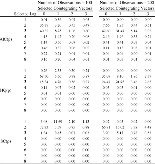
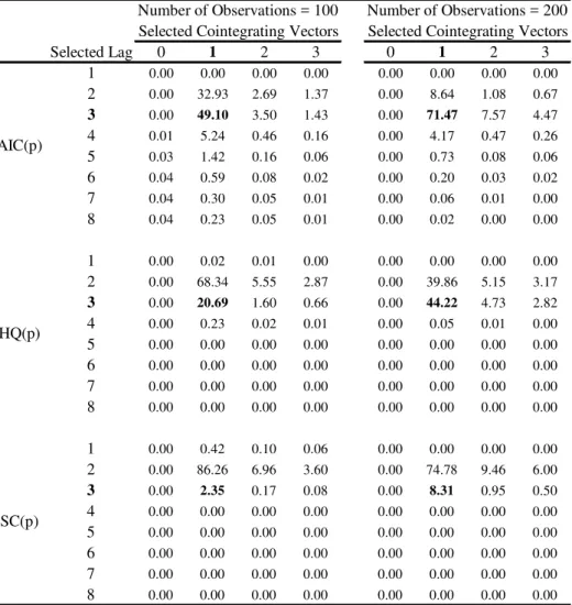
We now examine the performance of standard information criteria, followed by Johansen’s(1988, 1991) cointegrating test in selecting the number of lags of the VAR in levels p and the number of cointegrating vectors q when the DGP is a V AR(3) with r = 1, and q = 1. Table 2 shows the frequency of choice of p and q in 1,000 simulations of 100 trivariate VARs with a low system R2. Table 3 shows the same when systems with high R2s are considered.

We can draw the following conclusions from Tables 2 and 3. First, the total frequency in which the true lag length p = 3 is selected (adding up row 3 for all three IC(p)) varies very little with respect to the system R2_{, being about 50%, 20%, and 2%, for}

the DGP is (3;1), it is never the mode in Table 2, and is rarely the mode in Table 3. The performance of usingIC(p)to select pand q is discouraging for HQ(p) andSC(p): even when T = 200, and systemR2s are high, (p; q) = (3;1)is selected only 44.22% and 8.31% of times, respectively. Despite that, the frequency in which(3;1)is selected rises in both directions (sample size andR2 measure) as expected. Second, theAIC(p)criterium selects more frequently VARs where the number of lags is overestimated than the other criteria. This result is very similar to the one reported in Vahid and Issler(2002). Also, in Tables 2 and 3,AIC(p) chooses the correct(p; q) pairs more often than the other two criteria. The modal choice of the SC(p) criterium is a V AR(2) with one cointegrating vector even when the number of observations is 200 and the systemR2 _{is high.}

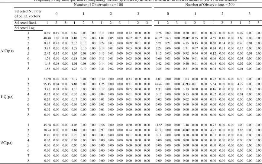
Table 4 shows the frequency of lag-rank-cointegrating vectors(p; r; q)selection in 1,000 simulations of 100 trivariateV AR(3)withr= 1, one cointegrating vector and low system

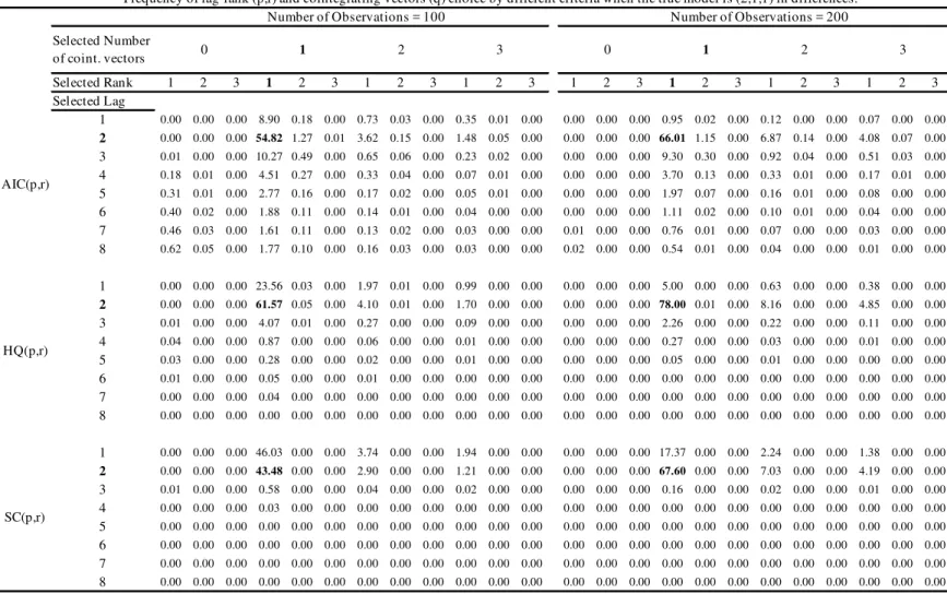
R2_{. There are two steps in this selection: (i) chose the number of lags and rank} simul-taneously byAIC(p; r),HQ(p; r) andSC(p; r); and (ii) use this information to perform Johansen’s cointegrating test to select the number of cointegrating vectors after applying the algorithm described in Section 3. Table 5 shows the analogous results when a high systemR2 is considered.

The following conclusions emerge from analyzing Tables 4 and 5. First, the total frequency in which the true lag length (2 lags in di¤erences) is selected (adding up row 2 for all three IC(p; r)) varies very little with respect to theR2 of the system: it is about 60%, 67%, and 48%, forAIC(p; r), HQ(p; r) and SC(p; r), respectively, when T = 100, and about 78%, 91% and 78%, whenT = 200. These results are equal or better than those of standard information criteriaIC(p). The mode for the selected lag length is always the correct one – 2 lags in di¤erences – except forSC(p; r). Second, theAIC(p; r) criterium selects more frequently VARs where the number of lags is overestimated than the other criteria. In both tables,HQ(p; r) chooses the correct(p; q; r) triplets more often than the other two criteria, withSC(p; r) in second place. For high systemR2s, the modal choice of HQ(p; r) criterium is the correct one with a relatively high frequency. Third, for low system R2_{s, and sample size T = 100, the true model is selected about 8%, 10%, and} 8% of times using respectively AIC(p; r), HQ(p; r) and SC(p; r). For high system R2

measures, and sample sizeT = 200, these same frequencies are about 78%, 91% and 78%. When we compare the results in Tables 2 and 3 with those of Tables 4 and 5, it becomes apparent that using information criteria in selecting(p; r) jointly fares much better than selecting p alone. In Tables 1 and 2 the true model with p = 3 and q = 1 is selected by AIC(p), HQ(p) and SC(p) respectively with frequency ranging from 8%-71%, 4%-44%, and 1%-8%. The equivalent …gures in Tables 4 and 5 for AIC(p; r), HQ(p; r) and

SC(p; r) are: 8%-66%, 10%-78%, and 8%-68%. The only instance when IC(p) performs better thanIC(p; r)is whenAIC( )is used. Even then, di¤erences are rather small. The direction in whichIC(p)performs badly is also worrisome, since the rule is for IC(p) to choose too small a lag length, leading to models with inconsistent estimates.

vec-tors. As discussed in previous theoretical and applied studies, if data have unit roots, selecting them appropriately is critical for consistent estimation and forecasting e¢ciency; see Johansen(1991), Gonzalo(1994), Clements and Hendry(1995) and Lin and Tsay(1996). However, the latter is jeopardized by the traditional way of model selection under coin-tegration and SCCF restrictions, which calls for a di¤erent approach – selecting lag and rank simultaneously usingIC(p; r).

5.3 Forecasts

In this section, we compare the forecasting performance of three di¤erent estimation pro-cedures for VARs containing short- and log-term restrictions. The …rst is to estimate the system in levels with no restrictions using OLS, equation-by equation. Lag length is selected using standard information criteria. The second is to select lag length using stan-dard information criteria, later imposing long-term restrictions arising from cointegration, and estimating a VECM. The third is to impose simultaneously short- and log-term re-strictions in VECM estimation using the algorithm described in Section 3, after selecting lag length and the rank of simultaneously.

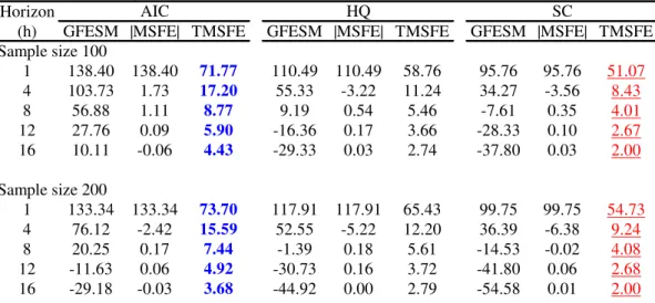
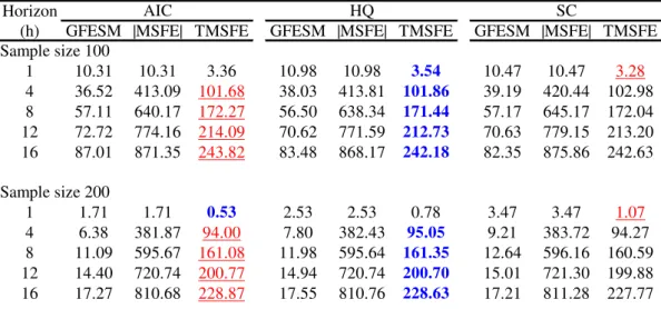
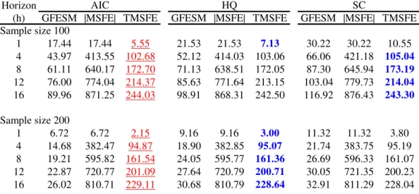
Tables 6 to 11 exhibit pairwise percentage improvement in forecasting for di¤erent models, when we consider systems with low and high R2s. Numbers in boldface denote the best information criterium for model selection when we use as loss function the trace of the mean-squared forecast error (lowest value), while underlined numbers denote the worst information criterium for model selection.

When we compare reduced-rank VECMs with unrestricted VECMs, we observe large percentage improvements at short horizons. These are really impressive – as big as 138% – when systemR2s are high andT = 100. Even whenR2s are low andT = 100, we observe percentage improvements ranging from 7%-20% for reduced-rank VECMs over VECMs.

When we compare the VECM with the unrestricted VAR we observe that the former fares better in general, although when system R2s are high, and the horizon is low, the unrestricted VAR performs better. Unless one uses GFESM, as the horizon increases, the percentage gains of the VECM over the unrestricted VAR increases, reaching more than 800% in some cases. Of course, this is a consequence of imposing long-term restrictions as stressed by Engle and Yoo(1987). In Tables 8 and 9 there is a large forecasting improve-ment over all horizons when theR2 _{measure is low, opposite to the …ndings in Engle and} Yoo. Of course, this is reverted when R2_{s are high, showing that their results hold only} as a special case as discussed in Section 5.1.

It is hard to use the results in Tables 6 to 11 to choose overall the best information criterium to use for lag-length selection. However, if one suspects that the data has SCCF and cointegration restrictions, then the HQ criterium should be used if the system R2

is low, while AIC should be used if the system R2 is high. The worst criterium to use in the …rst case is AIC, while in the second case it is SC. Notice that using HQ avoids selecting the worst models for forecasting, which may be a deciding factor in its favor. If one is considering only long-term restrictions AIC should be avoided, since it produces the largest loss overall. A strong candidate to be used here is the HQ criterium, especially if the systemR2 is low.

non-trivial at all horizons, reaching over 800% in some cases. The exception is when the system R2 measures are high and the horizons are lowest, although as it increases gains can reach more than 600%.

Overall, it seems that considering appropriately constrained models helps in forecast-ing. These gains can be important in short horizons, especially when high systemR2s are considered. As seen above, the gains in imposing long-term restrictions only materialize as the horizon increases, while those of imposing short-term restrictions are usually obtained at short-horizons. Because forecasting uncertainty at long horizons can be large, time-series models are generally most useful for forecasting at short horizons. Hence, imposing short-term constraints are a way of improving the e¤ectiveness of time-series models at horizons where they are most useful. This is one of the main points of our paper, which is not stressed very often in the forecasting literature. The other is the comparison of the gains arising from imposing short- and long-term restrictions in VAR estimation, which came always in favor of imposing short-term restrictions, with or without considering the possibility of misspeci…ed models.

6

Estimation performance of the new estimation algorithm

Our last investigation is on the performance of the new estimation algorithm, described in detail in Section 3. To save space, our simulation study will not be as broad as the one presented above in the forecasting experiment. Instead of …xing and e, solving analytically for Ai, i = 1;2; ; p, imposing the restriction that all the eigenvalues of the companion matrix of the VECM to be inside the unit circle, we …xed the restricted VECM coe¢cients (equation (5)), varying them slightly, verifying whether the eigenvalues of the companion matrix of the VECM are inside the unit circle in every case. To limit further the scope of our simulation study, we will assume that the lag length of the VAR

(p), the cointegrating rank(q) and the coefeature rank(n r) are known with certainty. Therefore, results here do not allow for model misspeci…cation, and are consistent with those presented in Table 1.

We will examine the mean-squared error (MSE) in estimating short- and long-term coe¢cients in the VAR. In all DGPs, the VAR in levels is assumed to be of order 2, i.e., a VECM of order 1. The number of variables in the VAR was set equal to 3, i.e.,n= 3, and we have varied q and r with all possible combinations: q = 1 and r = 1, q = 1and

r= 2, andq= 2andr = 2. In order to summarize MSE information we stack respectively short-term coe¢cients, long-term coe¢cients, and all coe¢cients in a vector, computing the determinant of the MSE matrix_jM SE_jas well as its trace(T M SE). We also report MSEs of individual coe¢cients.

First, MSE results were computed for VECMs, with cointegrating vectors estimated by FIML using Johansen’s(1988, 1991) technique, imposing the true value of q. Other coe¢cients were estimated by OLS, equation-by-equation. No reduced-rank structure for is imposed in this case. Second, MSE results were computed imposing a reduced-rank structure for , using the algorithm described in detail in Section 3: …rst estimate

short-term coe¢cients imposing rank( ) = r, later estimating I

p

P

i=1

percentage gains in MSE measures of the second procedure over the …rst for every DGP, …nally averaging across all DGPs. We have 100 di¤erent DGPs, each with 1,000 di¤erent simulations. Results are grouped by systemR2s.

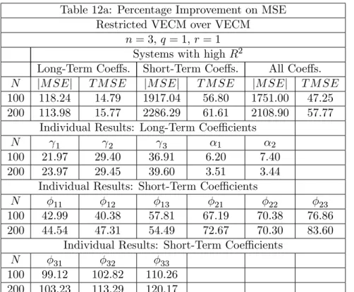
Table 12 (a and b) presents results for q = 1 and r = 1. Here, rank reduction is the highest possible, leading to a relatively high payo¤ of imposing rank restrictions in . As expected, estimation of short-term coe¢cients largely bene…t from correctly imposing

r = 1. For high system R2_{s, percentage gains in T M SE are higher than 50% when}

T = 100, and higher than 60% when T = 200. For low system R2s, these numbers are about 40%. What is interesting about Table 12, is the percentage gain on the T M SE

of long-term coe¢cients: with high system R2_{s, for T = 100 orT = 200 they are about} 15%, showing that long-term coe¢cient estimation can also bene…t from imposing valid short-term restrictions. It also interesting to observe that estimates bene…t the most, while for estimates of 0 _{the gains are more modest. This is a consequence of the fact that}

estimates of 0 using FIML are super-consistent. When systemR2s are low, there is a loss of about 7% in estimating 1 for T = 100, which reverts to a 4.86% gain for T = 200. Notice that results for_jM SE_jcompound variance and covariance gains, leading to much higher percentage gains.

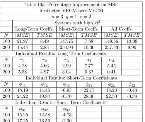
Table 13 (a and b) presents results for q = 1 and r = 2, while Table 14 (a and b) presents results forq= 2 and r= 2. We should expect a smaller percentage gain because there are not as many restrictions in as in the case where r = 1. Still, in Table 13, long-term coe¢cient estimates show an improvement inT M SEof 8.5% forT = 100, when systemR2_{s are high, falling to 6.5%, when systemR}2_{s are low. Improvement in short-term} coe¢cient estimates are also sizable, despite the fact that we observe a few cases where there is a loss in using the algorithm. In Table 14, we present long-term coe¢cients in canonical echelon form, since the cointegrating rank is now 2. In this case, improvement in

T M SEfor long-term coe¢cients are 19.79% for T = 100, when systemR2_{s are high, and} 20.55%, when system R2s are low. Gains for short run coe¢cients measured by T M SE

can reach more than 200% when systemR2s are low, and more than 300% when system

R2_{s are high.}

Overall, it seems that the new algorithm performs very well not only in estimating short-term coe¢cients but also in estimating long-term coe¢cients. This is a consequence of the fact that long-term coe¢cients are a cumulation of short-term coe¢cients. There-fore, gains in estimating the latter can translate into gains in estimating the former. Fur-ther research should focus on the long due issue of joint estimation of short- and long-term parameter estimation when VAR models are subject to short- and long-term restrictions.

7

Conclusion

Hecq, Palm and Urbain(2005) and Hecq(2005) …nd common cycles for Latin American GDPs. In all these articles, the dynamic representation of the data was a cointegrated VAR. A natural question which then arises is the following: what are the consequences of imposing short- and long-term restrictions in estimation and forecasting if a VAR is used as the dynamic representation of the data? The objective of our paper is to answer this question, hoping that the answer will be useful for model building.

In order to investigate these issues, we take VAR models, which have become the “working horses” for macroeconometric studies, and investigate the potential gains for forecasting and estimation uncertainty of imposing short- and long-term restrictions arising from the existence of common cycles and cointegration. The environment of our study is that of simulation, and our exercise is devised in such a way that the results are applicable to an applied researcher which has access to a relatively small number of time-series of observations, making parsimony a critical issue in model building.

In model selection and forecasting, we compare the behavior of the two strategies. The …rst is widely employed in applied work: VAR order is selected by standard information criteriaIC(p)and later used in testing for cointegration. The existence of common cycles is completely ignored and forecasting is performed with a standard VECM. The second takes into account short- and long-term restrictions in a novel way. In a …rst step, in-formation criteriaIC(p; r) are used to choose lag length and rank order simultaneously. Next, weak-form SCCF restrictions on VECM coe¢cient matrices are used in devising a new algorithm for joint estimation of short- and long-term parameters of the VAR. Fore-casting is based on a …nal model taking into account these two sets of restrictions. We also compare the estimation performance of these two strategies in model building, where short- and long-term parameters are considered separately.

First, our results con…rm that, when data have cointegration and SCCF restrictions, ignoring the latter has a high cost in terms of model selection. This happens becauseIC(p)

chooses too frequently inconsistent models, with too small a lag length. Choosing lag and rank simultaneously using IC(p; r) has a superior performance in this case, reducing drastically the frequency in which inconsistent models are selected. Second, the superior performance of IC(p; r) over IC(p) translates into a superior forecasting performance of the restricted VECM over the VECM, with considerable gains in some cases. Our conclusion is that, overall, there is a relatively large forecasting improvement for small horizons when SCCF restrictions are accounted for. Results for systems with high R2

measures are really impressive. Third, the new algorithm proposed here fares very well in terms of parameter estimation, even when we consider the estimation of long-term parameters.

References

[1] Ahn, S.K. and G.C. Reinsel (1988), “Nested reduced-rank autoregressive models for multiple time series”, Journal of the American Statistical Association, 83, 849-856.

[2] Beveridge, S. and C.R. Nelson (1981), “A New Approach to Decomposition of Eco-nomic Time Series into a Permanent and Transitory Components with Particular Attention to Measurement of the “Business Cycle”,Journal of Monetary Economics, vol. 7, pp. 151-174.

[3] Campbell, J.Y. and Mankiw, N.G.(1989), “Consumption, Income and Interest Rates: Reinterpreting the Time Series Evidence,” NBER Macroeconomics Annual.

[4] Carlino, G. and K. Sill (1998), “Common trends and common cycles in regional per-capita incomes”, Working Paper, Federal Reserve Bank of Philadelphia.

[5] Cheung, Y.W. and Lai, K.S. (1993), “Finite-samples sizes of johansen likelihood ratio tests for cointegration,”Oxford Bulletin of Economics and Statistics, 55 (3): 313-328.

[6] Christo¤ersen, P.F. and Diebold, F.X. (1998), “Cointegration and long-horizon fore-casting,” Journal of Business and Economic Statistics, vol. 16, 4, pp. 450-458.

[7] Clements, M.P. and D.F. Hendry (1993), “On the limitations of comparing mean squared forecast errors,” Journal of Forecasting, 12, 617-637 (with discussions).

[8] Clements, M.P. and D.F. Hendry (1995), “Forecasting in cointegrated systems”, Jour-nal of Applied Econometrics, 10, 127-146.

[9] Diebold, F.X. and Kilian L. (2001), “Measuring predictability: Theory and macro-economic applications,” Journal of Applied Econometrics, 16 (6): 657-669.

[10] Engle, R.F. and C.W.J. Granger (1987), “Cointegration and error correction: Repre-sentation, estimation and testing”, Econometrica, 55, 251-276.

[11] Engle, R.F. and J.V. Issler (1995), “Estimating common sectoral cycles”,Journal of Monetary Economics, 35, 83-113.

[12] Engle, R.F. and Kozicki, S.(1993), “Testing for Common Features,” Journal of Busi-ness and Economic Statistics, vol. 11, pp. 369-395, with discussions.

[13] Engle, R.F. and S. Yoo (1987), “Forecasting and testing in cointegrated systems”,

Journal of Econometrics, 35, 143-159.

[14] Gonzalo, J (1994), “Five alternative methods of estimating long-run equilibrium re-lationships,” Journal of Econometrics, 60 (1-2): 203-233.

[15] Granger, C.W.J.(1981), “Some properties of time series data and their use in econo-metric model speci…cation”, Journal of Econometrics, 16, pp. 121-130.

[17] Hecq, A., Palm, F.C., Urbain, J.-P. (2005), “Testing for common cyclical features in VAR models with cointegration,” forthcoming in the Annals Issue of the Journal of Econometrics on “Common Features.”

[18] Ho¤man, D.L. and Rasche, R.H. (1996), “Assessing forecast performance in a coin-tegrated system,” Journal of Applied Econometrics, 11 (5): 495-517.

[19] Issler, J.V. and Vahid, F. (2001), “Common Cycles and the Importance of Transitory Shocks to Macroeconomic Aggregates,”Journal of Monetary Economics,47, 449-475.

[20] Issler, J.V. and Vahid, F. (2005), “The Missing Link: Using the NBER Recession Indicator to Construct Coincident and Leading Indices of Economic Activity,” forth-coming in the Annals Issue of the Journal of Econometrics on “Common Features.”

[21] Johansen, S.(1988), “Statistical Analysis of Cointegrating Vectors,”Journal of Eco-nomic Dynamics and Control, vol. 12, pp. 231-254.

[22] Johansen, S.(1991), “Estimation and Hypothesis Testing of Cointegration Vectors in Gaussian Vector Autoregressive Models,”Econometrica, vol. 59, pp. 1551-1580.

[23] King, R., C.I. Plosser, J.H. Stock and M.W. Watson (1991), “Stochastic Trends and Economic Fluctuations”, American Economic Review, 81, 819-840.

[24] King, R.G., C.I. Plosser and S. Rebelo (1988), “Production, Growth and Business Cycles. II. New Directions,” Journal of Monetary Economics, vol. 21, pp. 309-341.

[25] Lin, J.L. and R.S. Tsay (1996), “Cointegration constraints and forecasting: An em-pirical examination”, Journal of Applied Econometrics,11, 519-538.

[26] Lütkepohl, H. (1985), “Comparison of criteria for estimating the order of a vector autoregressive process”, Journal of Time Series Analysis, 6, 35-52.

[27] Stock, J.H. and M.W. Watson (1988), “Testing for common trends”, Journal of the American Statistical Association, 83, 1097-1107.

[28] Silverstovs, B., Engsted T. and Haldrup N. (2004), “Long-run forecasting in multi-cointegrated systems,” Journal of Forecasting, 23 (5): 315-335.

[29] Stock, J. and Watson, M.(1989) “New Indexes of Leading and Coincident Economic Indicators”, NBER Macroeconomics Annual, 351-95.

[30] Tiao, G.C. and R.S. Tsay (1989), “Model speci…cation in multivariate time series (with discussions)”, Journal of the Royal Statistical Society, Series B, 51, 157-213.

[31] Tso, M.K-S. (1981), “Reduced rank regression and Canonical analysis” Journal of the Royal Statistical Society, Series B, 43, 183-189.

[32] Vahid, F. (1999), “A property of the companion matrix of a reduced rank VAR”,

Econometric Theory, 15, 787-788.

[34] Vahid, F. and Engle, R. (1997), “Codependent cycles,” Journal of Econometrics, 80 (2): 199-221.

[35] Vahid, F. and Issler, J.V. (2002), “The importance of common cyclical features in VAR analysis: A Monte Carlo study,” Journal of Econometrics, 109 (2): 341-363.

A

VAR restrictions for the DGPs

Consider the followingV AR(3) in levels:

yt=A1yt 1+A2yt 2+A3yt 3+"t; which can be rewritten as the followingV AR(1)process,

2 4 yytt1

0_yt

3

5=

2

4 (A2I3+A3) 0A3 0

0_(A2+A3) 0_A3 0 _{+ 1}

3 5

2 4 yytt 12

0_{yt 1}

3

5+

2 4 "0t

0_"t

3

5; (23)

where, 0 = (A1 +A2 +A3 I3); e =

2

4 e_e11₂₁ e_e12₂₂

e31 e32

3

5; =

2

4 11₂₁

31

3

5; =

2 4 11₂₁

31

3

5;

A2 =

2

4 a

2

11 a212 a213

a2

21 a222 a223

a2₃₁ a2₃₂ a2₃₃

3

5and A3 =

2

4 a

3

11 a312 a313

a3

21 a322 a323

a3₃₁ a3₃₂ a3₃₃

3 5.

It is helpful to de…ne,

t=

2 4 yytt1

0_yt

3

5; F =

2

4 (A2I3+A3) 0A3 0

0_(A2+A3) 0_A3 0 _{+ 1}

3

5 and t=

2 4 "0t

0_"t

3

5;

to arrive at,

t=F t 1+ t: (24)

If we consider cointegration and common-cycle restrictions, the following relations hold:

(i) _e0A3 = 0 ) A3 =

2 4

Ga3₃₁ Ga3₃₂ Ga3₃₃ Ka3

31 Ka332 Ka333

a3₃₁ a3₃₂ a3₃₃

3

5; where G = [R21K+R31]; K =

(R32 R31)=(R21 R22); Ri1=ei1=e11 and Ri2=ei2=e12 (i= 2;3); (ii) e0(A2+A3) = 0) e0A2= 0)A2=

2 4

Ga2

31 Ga232 Ga233

Ka2₃₁ Ka2₃₂ Ka2₃₃ a2₃₁ a2₃₂ a2₃₃

3 5;

(iii) _e0 = 0₎ =

2 4 KG 31₃₁

31

3

5;

(iv) 0_{(A2+A3) = (a}2

31+a331)S (a232+a323 )S (a233+a333)S and

0_{A3= a}3

31S a332S a333S ;whereS = 11G+ 21K+ 31; (v) 0 + 1 = ₃₁S+ 1:

The restrictions above imply that:

F = 2 6 6 6 6 6 6 6 6 4

G(a2₃₁+a3₃₁) G(a2₃₂+a3₃₂) G(a2₃₃+a3₃₃) Ga3₃₁ Ga3₃₂ Ga3₃₃ G ₃₁ K(a2₃₁+a3₃₁) K(a2₃₂+a3₃₂) K(a2₃₃+a3₃₃) Ka3₃₁ Ka3₃₂ Ka3₃₃ K ₃₁

(a2

31+a331) (a232+a332) (a233+a333) a331 a332 a333 31

1 0 0 0 0 0 0

0 1 0 0 0 0 0

0 0 1 0 0 0 0

(a2

31+a331)S (a322 +a332)S (a233+a333)S a331S a332S a333S 31S+ 1

If all the eigenvalues of matrixF lie inside the unit circle, then the VAR (24) is covariance-stationary. The eigenvalue of the matrix F is a number such that

jF I7j= 0: (25)

The solution of (25) is:

0 = 7 (1 + ₃₁S) a3₃₃+a3₃₂K+a₃₁3 G a2₃₃+a₃₂2 K+a2₃₁G 6 (26)

a2₃₃+a2₃₂K+a2₃₁G 5 a3₃₃+a3₃₂K+a3₃₁G 4:

If we de…ne = (1 + ₃₁S) a3₃₃+a3₃₂K+a3₃₁G a2₃₃+a2₃₂K+a2₃₁G ,

= a2₃₃+a2₃₂K+a2₃₁G and = a3₃₃+a3₃₂K+a3₃₁G , (26) is:

7₊ 6₊ 5₊ 4 _{= 0: (27)}

The roots of this polynomial are 1 = 2 = 3 = 4 = 0; 5 = A+B ₃; 6 =

A! +B!2 ₃; 7 = A!2 +B! ₃; where, ! = 1+

2 p

3 2 ; A =

3

r

b2

2 +

2

q

b2

4 + a3

27;

B = 3

r

b2

2

2

q

b2

4 +a

3

27; a= 13 3 2 andb= 271 2 3 9 + 27 .

B

Tables

Horizon

(h) GFESM |MSFE| TMSFE GFESM |MSFE| TMSFE GFESM |MSFE| TMSFE

Sample size 100

1 5.11 5.11 1.67 16.40 16.40 5.34 11.28 11.28 3.68

4 20.48 407.50 99.96 44.55 409.99 102.33 24.06 2.50 2.37

8 33.39 635.26 171.01 60.44 635.99 172.38 27.06 0.73 1.37

12 44.08 769.22 212.98 72.74 769.63 213.95 28.66 0.41 0.97

16 54.73 866.74 242.75 84.61 867.05 243.51 29.89 0.31 0.76

Sample size 200

1 1.92 1.92 0.62 7.30 7.30 2.38 5.38 5.38 1.76

4 7.50 381.37 93.96 17.99 382.16 94.99 10.49 0.79 1.03

8 12.66 594.71 161.02 24.21 594.91 161.59 11.56 0.20 0.57

12 16.12 719.71 200.69 28.26 719.84 201.08 12.14 0.13 0.40

16 19.20 809.72 228.77 31.71 809.75 229.07 12.51 0.03 0.30

Sample size 100

1 -165.41 -165.41 -85.26 -30.33 -30.33 -13.73 135.08 135.08 71.53

4 -278.95 275.06 49.22 -197.63 273.60 64.62 81.32 -1.46 15.40

8 -321.63 442.14 103.05 -288.41 443.31 110.86 33.22 1.17 7.81

12 -330.03 537.34 138.04 -323.14 537.74 143.33 6.89 0.39 5.29

16 -325.15 607.36 165.11 -330.58 607.47 169.10 -5.43 0.11 3.98

Sample size 200

1 -169.09 -169.09 -88.58 -40.54 -40.54 -16.87 128.55 128.55 71.72

4 -287.72 261.16 45.16 -230.40 256.60 58.97 57.33 -4.56 13.80

8 -336.24 421.61 97.18 -334.98 421.94 103.68 1.25 0.33 6.50

12 -350.81 512.31 130.20 -379.24 512.47 134.52 -28.43 0.15 4.33

16 -352.76 577.82 155.52 -395.17 577.84 158.76 -42.41 0.02 3.24

GFESM is Clements and Hendry's generalized forecast error second moment measure, |MSFE| is the determinant of the of the mean squared forecast error matrix and TMSFE is the trace of the MSFE matrix.

High system R2 Measure Table 1

Percentage improvement in different forecast accuracy measures when the true restrictions (lags, rank and number of cointegrated vectors) are imposed and the true models are trivariate (3,1,1).

VECM over VAR in levels Reduced-rank VECM over the VAR in levels

Reduced-rank VECM over the VECM

Selected Lag 0 1 _{2 3 0} 1 _{2 3} 1 0.01 0.36 0.07 0.05 0.00 0.00 0.00 0.00

2 35.79 3.20 0.45 0.47 7.66 1.85 0.44 0.51

3 40.32 8.23 1.06 0.60 42.60 31.47 5.14 3.98

4 4.13 1.42 0.20 0.08 2.46 1.96 0.35 0.24 5 1.14 0.56 0.07 0.02 0.41 0.41 0.07 0.04 6 0.46 0.32 0.06 0.02 0.11 0.13 0.03 0.01 7 0.27 0.21 0.04 0.01 0.04 0.04 0.00 0.01 8 0.16 0.20 0.04 0.01 0.01 0.03 0.01 0.00

1 0.26 2.53 0.50 0.24 0.00 0.00 0.00 0.00

2 68.50 5.66 0.78 0.87 35.07 8.10 1.86 2.39

3 15.34 4.26 0.56 0.27 24.47 21.95 3.46 2.63

4 0.14 0.07 0.02 0.00 0.03 0.03 0.01 0.00 5 0.01 0.01 0.00 0.00 0.00 0.00 0.00 0.00 6 0.00 0.00 0.00 0.00 0.00 0.00 0.00 0.00 7 0.00 0.00 0.00 0.00 0.00 0.00 0.00 0.00 8 0.00 0.00 0.00 0.00 0.00 0.00 0.00 0.00

1 3.08 11.69 2.10 1.13 0.02 0.05 0.02 0.00

2 72.73 5.59 0.75 0.88 66.71 15.02 3.38 4.48

3 1.34 0.63 0.07 0.03 3.90 5.12 0.78 0.53 4 0.00 0.00 0.00 0.00 0.00 0.00 0.00 0.00 5 0.00 0.00 0.00 0.00 0.00 0.00 0.00 0.00 6 0.00 0.00 0.00 0.00 0.00 0.00 0.00 0.00 7 0.00 0.00 0.00 0.00 0.00 0.00 0.00 0.00 8 0.00 0.00 0.00 0.00 0.00 0.00 0.00 0.00

Numbers represent the percentage times that the model selection criterion chose that cell, corresponding to the lag and number of cointegrating vectors, in 100,000 times (1000 simulations of 100 different DGPs). The true lag-cointegrating vectors are indentified by bold numbers.

HQ(p)

SC(p)

Table 2 - Low system R2 Measure

Frequency of lag (p) and cointegrating vectors (q) choice by different criteria when the true model is (3,1,1) in levels.

Selected Cointegrating Vectors

AIC(p)

Selected Lag 0 1 _{2 3 0} 1 _{2 3} 1 0.00 0.00 0.00 0.00 0.00 0.00 0.00 0.00

2 0.00 32.93 2.69 1.37 0.00 8.64 1.08 0.67

3 0.00 49.10 3.50 1.43 0.00 71.47 7.57 4.47

4 0.01 5.24 0.46 0.16 0.00 4.17 0.47 0.26 5 0.03 1.42 0.16 0.06 0.00 0.73 0.08 0.06 6 0.04 0.59 0.08 0.02 0.00 0.20 0.03 0.02 7 0.04 0.30 0.05 0.01 0.00 0.06 0.01 0.00 8 0.04 0.23 0.05 0.01 0.00 0.02 0.00 0.00

1 0.00 0.02 0.01 0.00 0.00 0.00 0.00 0.00

2 0.00 68.34 5.55 2.87 0.00 39.86 5.15 3.17

3 0.00 20.69 1.60 0.66 0.00 44.22 4.73 2.82

4 0.00 0.23 0.02 0.01 0.00 0.05 0.01 0.00 5 0.00 0.00 0.00 0.00 0.00 0.00 0.00 0.00 6 0.00 0.00 0.00 0.00 0.00 0.00 0.00 0.00 7 0.00 0.00 0.00 0.00 0.00 0.00 0.00 0.00 8 0.00 0.00 0.00 0.00 0.00 0.00 0.00 0.00

1 0.00 0.42 0.10 0.06 0.00 0.00 0.00 0.00

2 0.00 86.26 6.96 3.60 0.00 74.78 9.46 6.00

3 0.00 2.35 0.17 0.08 0.00 8.31 0.95 0.50 4 0.00 0.00 0.00 0.00 0.00 0.00 0.00 0.00 5 0.00 0.00 0.00 0.00 0.00 0.00 0.00 0.00 6 0.00 0.00 0.00 0.00 0.00 0.00 0.00 0.00 7 0.00 0.00 0.00 0.00 0.00 0.00 0.00 0.00 8 0.00 0.00 0.00 0.00 0.00 0.00 0.00 0.00 SC(p)

Numbers represent the percentage times that the model selection criterion chose that cell, corresponding to the lag and number of cointegrating vectors, in 100,000 times (1000 simulations of 100 different DGPs). The true lag-cointegrating vectors are indentified by bold numbers.

Selected Cointegrating Vectors Selected Cointegrating Vectors

AIC(p)

HQ(p)

Table 3 - High system R2 Measure

Frequency of lag (p) and cointegrating vectors (q) choice by different criteria when the true model is (3,1,1) in levels.

3 0.00 0.00 0.00 0.00 0.00 0.00 0.00 0.00 0.00 0.00 0.00 0.00 0.00 0.00 0.00 0.00 0.00 0.00 0.00 0.00 0.00 0.00 0.00 0.00 2 0.00 0.08 0.01 0.00 0.01 0.00 0.00 0.00 0.00 0.00 0.00 0.00 0.00 0.00 0.00 0.00 0.00 0.00 0.00 0.00 0.00 0.00 0.00 0.00 1 0.07 3.60 0.40 0.13 0.06 0.03 0.02 0.01 0.30 4.29 0.10 0.01 0.00 0.00 0.00 0.00 1.00 3.83 0.00 0.00 0.00 0.00 0.00 0.00 3 0.00 0.00 0.00 0.00 0.00 0.00 0.00 0.00 0.00 0.00 0.00 0.00 0.00 0.00 0.00 0.00 0.00 0.00 0.00 0.00 0.00 0.00 0.00 0.00 2 0.00 0.10 0.04 0.01 0.00 0.00 0.00 0.00 0.00 0.00 0.00 0.00 0.00 0.00 0.00 0.00 0.00 0.00 0.00 0.00 0.00 0.00 0.00 0.00 1 0.05 4.55 0.60 0.24 0.12 0.06 0.04 0.04 0.22 5.54 0.16 0.02 0.01 0.00 0.00 0.00 0.77 4.97 0.01 0.00 0.00 0.00 0.00 0.00 3 0.00 0.00 0.00 0.00 0.00 0.00 0.00 0.00 0.00 0.00 0.00 0.00 0.00 0.00 0.00 0.00 0.00 0.00 0.00 0.00 0.00 0.00 0.00 0.00 2 0.01 0.55 0.15 0.07 0.04 0.01 0.01 0.00 0.00 0.01 0.00 0.00 0.00 0.00 0.00 0.00 0.00 0.00 0.00 0.00 0.00 0.00 0.00 0.00 1 0.20 28.07 4.15 1.71 0.92 0.56 0.40 0.31 1.03 33.93 1.13 0.15 0.02 0.00 0.00 0.00 3.48 30.87 0.10 0.00 0.00 0.00 0.00 0.00 3 0.00 0.00 0.00 0.00 0.00 0.00 0.00 0.00 0.00 0.00 0.00 0.00 0.00 0.00 0.00 0.00 0.00 0.00 0.00 0.00 0.00 0.00 0.00 0.00 2 0.02 0.63 0.21 0.06 0.03 0.01 0.01 0.01 0.00 0.01 0.00 0.00 0.00 0.00 0.00 0.00 0.00 0.00 0.00 0.00 0.00 0.00 0.00 0.00 1 0.76 40.25 5.71 2.24 1.15 0.69 0.42 0.35 4.03 47.49 1.33 0.17 0.03 0.00 0.00 0.00 14.55 40.30 0.11 0.00 0.00 0.00 0.00 0.00 3 0.00 0.00 0.00 0.00 0.00 0.00 0.00 0.00 0.00 0.00 0.00 0.00 0.00 0.00 0.00 0.00 0.00 0.00 0.00 0.00 0.00 0.00 0.00 0.00 2 0.00 0.02 0.01 0.00 0.00 0.00 0.00 0.00 0.00 0.00 0.00 0.00 0.00 0.00 0.00 0.00 0.00 0.00 0.00 0.00 0.00 0.00 0.00 0.00 1 0.12 0.62 0.09 0.05 0.03 0.03 0.03 0.05 0.33 0.71 0.05 0.01 0.01 0.00 0.00 0.00 0.60 0.54 0.01 0.00 0.00 0.00 0.00 0.00 3 0.00 0.00 0.00 0.00 0.00 0.00 0.00 0.00 0.00 0.00 0.00 0.00 0.00 0.00 0.00 0.00 0.00 0.00 0.00 0.00 0.00 0.00 0.00 0.00 2 0.00 0.05 0.03 0.01 0.01 0.01 0.01 0.02 0.00 0.00 0.00 0.00 0.00 0.00 0.00 0.00 0.00 0.00 0.00 0.00 0.00 0.00 0.00 0.00 1 0.11 1.01 0.24 0.14 0.13 0.11 0.14 0.21 0.30 1.25 0.12 0.04 0.01 0.01 0.01 0.00 0.56 0.97 0.03 0.00 0.00 0.00 0.00 0.00 3 0.00 0.00 0.00 0.00 0.00 0.00 0.00 0.00 0.00 0.00 0.00 0.00 0.00 0.00 0.00 0.00 0.00 0.00 0.00 0.00 0.00 0.00 0.00 0.00 2 0.03 0.29 0.13 0.10 0.08 0.08 0.08 0.10 0.01 0.02 0.00 0.00 0.00 0.00 0.00 0.00 0.00 0.00 0.00 0.00 0.00 0.00 0.00 0.00 1 0.82 8.06 2.16 1.28 1.07 0.88 1.01 1.23 2.17 9.88 1.10 0.35 0.17 0.04 0.04 0.00 4.08 7.87 0.20 0.02 0.00 0.00 0.00 0.00 3 0.00 0.01 0.00 0.00 0.00 0.00 0.00 0.00 0.00 0.00 0.00 0.00 0.00 0.00 0.00 0.00 0.00 0.00 0.00 0.00 0.00 0.00 0.00 0.00 2 0.19 1.08 0.42 0.20 0.12 0.09 0.08 0.07 0.02 0.04 0.01 0.00 0.00 0.00 0.00 0.00 0.00 0.00 0.00 0.00 0.00 0.00 0.00 0.00 1 8.69 48.48 8.83 3.83 2.42 1.74 1.45 1.58 23.50 55.15 3.45 0.72 0.25 0.04 0.02 0.00 45.68 38.94 0.46 0.02 0.00 0.00 0.00 0.00 Selected Number of coint. vectors Selected Rank Selected Lag 1 2 3 4 5 6 7 8 1 2 3 4 5 6 7 8 1 2 3 4 5 6 7 8

Number of Observations = 200 Frequency of lag-rank (p,r) and cointegrating vectors (q) choice by different criteria when the true model is (2,1,1) in differences.

Table 4 - Low system R2 Measure

AIC(p,r)

HQ(p,r)

SC(p,r)

Number of Observations = 100

3

2 2 3

1

0 0 1