❊♥s❛✐♦s ❊❝♦♥ô♠✐❝♦s
❊s❝♦❧❛ ❞❡
Pós✲●r❛❞✉❛çã♦
❡♠ ❊❝♦♥♦♠✐❛
❞❛ ❋✉♥❞❛çã♦
●❡t✉❧✐♦ ❱❛r❣❛s
◆◦ ✻✽✽ ■❙❙◆ ✵✶✵✹✲✽✾✶✵
▼♦❞❡❧ s❡❧❡❝t✐♦♥✱ ❡st✐♠❛t✐♦♥ ❛♥❞ ❢♦r❡❝❛st✐♥❣
✐♥ ❱❆❘ ♠♦❞❡❧s ✇✐t❤ s❤♦rt✲r✉♥ ❛♥❞ ❧♦♥❣✲r✉♥
r❡str✐❝t✐♦♥s
●❡♦r❣❡ ❆t❤❛♥❛s♦♣♦✉❧♦s✱ ❖s♠❛♥✐ ❚❡✐①❡✐r❛ ❈❛r✈❛❧❤♦ ●✉✐❧❧é♥✱ ❏♦ã♦ ❱✐❝t♦r ■ss❧❡r✱ ●❡♦r❣❡ ❆t❤❛♥❛s♦♣♦✉❧♦s
❖s ❛rt✐❣♦s ♣✉❜❧✐❝❛❞♦s sã♦ ❞❡ ✐♥t❡✐r❛ r❡s♣♦♥s❛❜✐❧✐❞❛❞❡ ❞❡ s❡✉s ❛✉t♦r❡s✳ ❆s
♦♣✐♥✐õ❡s ♥❡❧❡s ❡♠✐t✐❞❛s ♥ã♦ ❡①♣r✐♠❡♠✱ ♥❡❝❡ss❛r✐❛♠❡♥t❡✱ ♦ ♣♦♥t♦ ❞❡ ✈✐st❛ ❞❛
❋✉♥❞❛çã♦ ●❡t✉❧✐♦ ❱❛r❣❛s✳
❊❙❈❖▲❆ ❉❊ PÓ❙✲●❘❆❉❯❆➬➹❖ ❊▼ ❊❈❖◆❖▼■❆ ❉✐r❡t♦r ●❡r❛❧✿ ❘❡♥❛t♦ ❋r❛❣❡❧❧✐ ❈❛r❞♦s♦
❉✐r❡t♦r ❞❡ ❊♥s✐♥♦✿ ▲✉✐s ❍❡♥r✐q✉❡ ❇❡rt♦❧✐♥♦ ❇r❛✐❞♦ ❉✐r❡t♦r ❞❡ P❡sq✉✐s❛✿ ❏♦ã♦ ❱✐❝t♦r ■ss❧❡r
❉✐r❡t♦r ❞❡ P✉❜❧✐❝❛çõ❡s ❈✐❡♥tí✜❝❛s✿ ❘✐❝❛r❞♦ ❞❡ ❖❧✐✈❡✐r❛ ❈❛✈❛❧❝❛♥t✐
❆t❤❛♥❛s♦♣♦✉❧♦s✱ ●❡♦r❣❡
▼♦❞❡❧ s❡❧❡❝t✐♦♥✱ ❡st✐♠❛t✐♦♥ ❛♥❞ ❢♦r❡❝❛st✐♥❣ ✐♥ ❱❆❘ ♠♦❞❡❧s ✇✐t❤ s❤♦rt✲r✉♥ ❛♥❞ ❧♦♥❣✲r✉♥ r❡str✐❝t✐♦♥s✴ ●❡♦r❣❡ ❆t❤❛♥❛s♦♣♦✉❧♦s✱ ❖s♠❛♥✐ ❚❡✐①❡✐r❛ ❈❛r✈❛❧❤♦ ●✉✐❧❧é♥✱ ❏♦ã♦ ❱✐❝t♦r ■ss❧❡r✱ ●❡♦r❣❡ ❆t❤❛♥❛s♦♣♦✉❧♦s ✕ ❘✐♦ ❞❡ ❏❛♥❡✐r♦ ✿ ❋●❱✱❊P●❊✱ ✷✵✶✵
✭❊♥s❛✐♦s ❊❝♦♥ô♠✐❝♦s❀ ✻✽✽✮ ■♥❝❧✉✐ ❜✐❜❧✐♦❣r❛❢✐❛✳
Model selection, estimation and forecasting in VAR models with
short-run and long-run restrictions
George Athanasopoulos
Department of Econometrics and Business Statistics Monash University
Clayton, Victoria 3800 Australia
Osmani Teixeira de Carvalho Guill´en Banco Central do Brasil and IBMEC-RJ
Av. Presidente Vargas, 730 - Centro Rio de Janeiro, RJ 20071-001
Brazil
Jo˜ao Victor Issler*
Graduate School of Economics – EPGE Getulio Vargas Foundation Praia de Botafogo 190 s. 1111
Rio de Janeiro, RJ 22253-900 Brazil
Farshid Vahid School of Economics
The Australian National University Canberra, ACT 0200
Australia
Jan 31, 2009
Abstract
We study the joint determination of the lag length, the dimension of the cointegrating space and the rank of the matrix of short-run parameters of a vector autoregressive (VAR) model using model selection criteria. We consider model selection criteria which have data-dependent penalties for a lack of parsimony, as well as the traditional ones. We suggest a new procedure which is a hybrid of traditional criteria and criteria with data-dependant penalties. In order to compute the fit of each model, we propose an iterative procedure to compute the maximum likelihood estimates of parameters of a VAR model with short-run and long-run restrictions. Our Monte Carlo simulations measure the improvements in forecasting accuracy that can arise from the joint determination of lag-length and rank, relative to the commonly used procedure of selecting the lag-length only and then testing for cointegration.
Keywords: Reduced rank models, model selection criteria, forecasting accuracy.
JEL Classification: C32, C53.
1
Introduction
There is a large body of literature on the effect of cointegration on forecasting. Engle and Yoo (1987)
compare the forecasts generated from an estimated VECM assuming that the lag order and the
coin-tegrating rank are known, with those from an estimated VAR in levels with the correct lag. They
find out that the VECM only produces forecasts with smaller mean squared forecast errors (MSFE)
in the long-run. Clements and Hendry (1995) note that Engle and Yoo’s conclusion is not robust if
the object of interest is differences rather than levels, and use this observation to motivate their
alter-native measures for comparing multivariate forecasts. Hoffman and Rasche (1996) confirm Clements
and Hendry’s observation using a real data set. Christoffersen and Diebold (1998) also use Engle and
Yoo’s setup, but argue against using a VAR in levels as a benchmark on the grounds that the VAR in
levels not only does not impose cointegration, it does not impose any unit roots either. Instead, they
compare the forecasts of a correctly specified VECM with forecasts from correctly specified univariate
models, and find no advantage in MSFE for the VECM. They use this result as a motivation to suggest
an alternative way of evaluating forecasts of a cointegrated system. Silverstovs et al. (2004) extend
Christoffersen and Diebold’s results to multicointegrated systems. Since the afore-mentioned papers
condition on the correct specification of the lag length and cointegrating rank, they cannot provide an
answer as to whether we should examine the cointegrating rank of a system in multivariate forecasting
if we do not have any a priori reason to assume a certain form of cointegration.
Lin and Tsay (1996) examine the effect on forecasting of the mis-specification of the cointegrating
rank. They determine the lag order using the AIC, and compare the forecasting performance of
estimated models under all possible numbers of cointegrating vectors (0 to 4) in a four-variable system.
They observe that, keeping the lag order constant, the model with the correct number of cointegrating
vectors achieves a lower MSFE for long-run forecasts, especially relative to a model that over-specifies
the cointegrating rank. Although Lin and Tsay do not assume the correct specification of the lag
length, their study also does not address the uncertainty surrounding the number of cointegrating
vectors in a way that can lead to a modelling strategy for forecasting possibly cointegrated variables.
Indeed, the results of their example with real data, in which they determine the cointegrating rank
using a sequence of hypothesis tests, do not accord with their simulation results.
At the same time, there is an increasing amount of evidence of the advantage of considering rank
restrictions for short-term forecasting in stationary VAR (and VARMA) models (see, for example, Ahn
and Reinsel, 1988; Vahid and Issler, 2002; Athanasopoulos and Vahid, 2008). One feature of these
papers is that they do not treat lag-length and rank uncertainty, differently. Their quest is to identify
Here, we add the cointegrating rank to the menu of unknowns and evaluate model selection criteria
that determine all of these unknowns simultaneously. Our goal is to determine a modelling strategy
that is useful for multivariate forecasting.
There are other papers in the literature that evaluate the performance of model selection criteria
for determining lag-length and cointegrating rank, but they do not evaluate the forecast performance
of the resulting models. Gonzalo and Pitarakis (1999) show that in large systems the usual model
selection procedures may severely underestimate the cointegrating rank. Chao and Phillips (1999)
show that the posterior information criterion (PIC) performs well in choosing the lag-length and the
cointegrating rank simultaneously.
In this paper we evaluate the performance of model selection criteria in the simultaneous choice
of the lag-length p, the rank of the cointegrating spaceq, and the rank of other parameter matricesr
in a vector error correction model. We suggest a hybrid model selection strategy that selects p and r
using a traditional model selection criterion, and then chooses q based on PIC. We then evaluate the
forecasting performance of models selected using these criteria.
Our simulations cover the three issues of model building, estimation, and forecasting. We examine
the performances of model selection criteria that choose p, r and q simultaneously (IC(p, r, q)), and
compare their performances with a procedure that choosespusing a standard model selection criterion
(IC(p)) and determines the cointegrating rank using a sequence of likelihood ratio tests proposed by
Johansen (1988). We provide a comparison of the forecasting accuracy of fitted VARs when only
coin-tegration restrictions are imposed, when coincoin-tegration and short-run restrictions are jointly imposed,
and when neither are imposed. These comparisons take into account the possibility of model
misspec-ification in choosing the lag length of the VAR, the number of cointegrating vectors, and the rank of
other parameter matrices. In order to estimate the parameters of a model with both long-run and
short-run restrictions, we propose a simple iterative procedure similar to the one proposed by Centoni
et al. (2007).
It is very difficult to claim that any result found in a Monte Carlo study is general, especially
in multivariate time series. There are examples in the VAR literature of Monte Carlo designs which
led to all model selection criteria overestimating the true lag in small samples, therefore leading to
the conclusion that the Schwarz criterion is the most accurate. The most important feature of these
designs is that they have a strong propagation mechanism.1 There are other designs with weak
propa-gation mechanisms that result in all selection criteria underestimating the true lag and leading to the
conclusion that AIC’s asymptotic bias in overestimating the true lag may actually be useful in finite
1
samples (see Vahid and Issler, 2002, for references). We pay particular attention to the design of the
Monte Carlo to make sure that we cover a wide range of data generating processes in terms of the
strength of their propagation mechanisms.
The outline of the paper is as follows. In Section 2 we study finite VARs with long-run and
short-run restrictions and motivate their empirical relevance. In Section 3, we outline an iterative procedure
for computing the maximum likelihood estimates of parameters of a VECM with short-run restrictions.
We provide an overview of model selection criteria in Section 4, and in particular we discuss model
selection criteria with data dependent penalty functions. Section 5 describes our Monte Carlo design.
Section 6 presents the simulation results and Section 8 concludes.
2
VAR models with long-run and short-run common factors
We start from the triangular representation of a cointegrated system used extensively in the
cointe-gration literature (some early examples are Phillips and Hansen, 1990; Phillips and Loretan, 1991;
Saikkonen, 1992). We assume that the K-dimensional time series
yt=
y1t y2t
, t= 1, ..., T
wherey1t isq×1 (implying thaty2tis (K−q)×1) is generated from:
y1t = βy2t+u1t (1)
∆y2t = u2t
whereβ is aq×(K−q) matrix of parameters, and
ut=
u1t u2t
is a strictly stationary process with mean zero and positive definite covariance matrix. This is a DGP
of a system ofK cointegrated I(1) variables withqcointegrating vectors, also referred to as a system of
K I(1) variables with K−q common stochastic trends (some researchers also refer to this as a system ofK variables withK−qunit roots, which can be ambiguous if used out of context, and we therefore do not use it here).2 The extra feature that we add to this fairly general DGP is that u
t is generated
from a VAR of finite order p and rankr (< K).
In empirical applications, the finite VAR(p) assumption is routine. This is in contrast to the
theoretical literature on testing for cointegration, in whichut is assumed to be an infinite VAR, and a
2
finite VAR(p) is used as an approximation (e.g. Saikkonen, 1992). Here, our emphasis is on building
multivariate forecasting models rather than hypothesis testing. The finite VAR assumption is also
routine when the objective is studying the maximum likelihood estimator of the cointegrating vectors,
as in Johansen (1988).
The reduced rank assumption is considered for the following reasons. Firstly, this assumption
means that all serial dependence in the K-dimensional vector time series ut can be characterised by
only r < K serially dependent indices. This is a feature of most macroeconomic models, in which
the short-run dynamics of the variables around their steady states are generated by a small number
of serially correlated demand or supply shifters. Secondly, this assumption implies that there are
K−r linear combinations ofut that are white noise. Gourieroux and Peaucelle (1992) call such time
series “codependent,” and interpret the white noise combinations as equilibrium combinations among
stationary variables. This is justified on the grounds that, although each variable has some persistence,
the white noise combinations have no persistence at all. For instance, if an optimal control problem
implies that the policy instrument should react to the current values of the target variables, then it is
likely that there will be such a linear relationship between the observed variables up to a measurement
noise. Finally, many papers in multivariate time series literature provide evidence of the usefulness
of reduced rank VARs for forecasting (see, for example, Velu et al., 1986; Ahn and Reinsel, 1988).
Recently, Vahid and Issler (2002) have shown that failing to allow for the possibility of reduced rank
structure can lead to developing seriously misspecified vector autoregressive models that produce bad
forecasts.
The dynamic equation for ut is therefore given by (all intercepts are suppressed to simplify the
notation)
ut=B1ut−1+B2ut−2+· · ·+Bput−p+εt (2)
whereB1, B2, ..., BpareK×Kmatrices withrank B1 B2 ... Bp =r, andεtis an i.i.d. sequence with mean zero and positive definite variance-covariance matrix and finite fourth moments. Note that
the rank condition implies that each Bi has rank at most r, and the intersection of the null-spaces
of all Bi is a subspace of dimension K −r. The following lemma derives the vector error correction representation of this data generating process.
Lemma 1 The data generating process given by equations (1) and (2) has a reduced rank vector error correction representation of the type
∆yt=γ Iq −β
yt−1+ Γ1∆yt−1+ Γ2∆yt−2+· · ·+ Γp∆yt−p+ηt, (3)
in which rank
Γ1 Γ2 ... Γp
Proof: See Appendix A.
This lemma shows that the triangular DGP (1) under the assumption that the dynamics of its
stationary component (i.e. ut) can be characterised by a small number of common factors, is equivalent
to a VECM in which the coefficient matrices of lagged differences have reduced rank and their left
null-spaces overlap. Hecq et al. (2006) call such a structure a VECM with weak serial correlation common
features (WSCCF). It is instructive here to compare this structure with a DGP that embodies a stricter
form of co-movement, namely one that implies that the dynamics of the deviations of yt from their
Beveridge-Nelson (BN) trends can be characterised by a small number of cyclical terms.
Starting from the Wold representation for ∆yt
∆yt= Θ(L)ηt,
where Θ(L) is an infinite moving average matrix polynomial with Θ0 =IK and absolutely summable
coefficients and ηt are innovations in ∆yt, then, using the matrix identity used in the proof of the
lemma above, we get
yt= Θ(1)
∞
X
i=0
ηt−i+ Θ∗(L)ηt,
where Θ∗j =−P∞
i=j+1Θi.The first term is the vector of BN trends. These are random walks, and are simply the limit of the long-run forecastyt+h|tash→ ∞.Cointegration implies that Θ(1) has reduced
rank, and hence the K random walk trends can be written in terms of a smaller number of common
BN trends. Specifically,qcointegrating vectors are equivalent toK−qcommon BN trends. Deviations from the BN trends, i.e. Θ∗(L)η
t, are usually called the BN “cycles”. The question is whether the
reduced rank structure assumed for ut in the triangular system above implies that the BN cycles can
be characterised as linear combinations of r common factors. And the answer is negative. Vahid and
Engle (1993) analyse the restrictions that common trends and common cycles impose on a VECM.
They show that, in addition to a rank restriction similar to the one derived above on the coefficients
of lagged differences, the left null-space of the coefficient of the lag level must also overlap with that of
all other coefficient matrices. That is, the DGP with common BN cycles is a special case of the above
under some additional restrictions.
One may question why we do not restrict our attention to models with common BN cycles, given
that the above reasons in support of the triangular structure, and in particular the fact that most macro
models imply that deviations from the steady state depend on a small number of common factors, more
compellingly support a model with common BN cycles. However, Hecq et al. (2006) show that the
uncertainty in determining the rank of the cointegrating space can adversely affect inference on common
means of uncovering short-run restrictions in vector error correction models. Therefore, as a systematic
approach to allow for more parsimonious models than the unrestricted VECMs, it seems imprudent to
consider only the strong form of serial correlation common features.
Our objective is to come up with a model development methodology that allows for cointegration
and weak serial correlation common features. For stationary time series, Vahid and Issler (2002) show
that allowing for reduced rank models is beneficial for forecasting. For partially non-stationary time
series, there is an added dimension of cointegration. Here, we examine the joint benefits of cointegration
and short-run rank restrictions for forecasting partially non-stationary time series.
3
Estimation of VARs with short-run and long-run restrictions
The maximum likelihood estimation of the parameters of a VAR written in error-correction form
∆yt= Πyt−1+ Γ1∆yt−1+ Γ2∆yt−2+· · ·+ Γp∆yt−p+ηt (4)
under the long-run restriction that the rank of Π is q, the short-run restriction that rank of
Γ1 Γ2 ... Γp
is r and the assumption of normality, is possible via a simple iterative
proce-dure that uses the general principle of the estimation of reduced rank regression models (Anderson,
1951). Noting that the above model can be written as
∆yt = γ α′yt−1+C[D1∆yt−1+D2∆yt−2+· · ·+Dp∆yt−p] +ηt, (5)
whereαis aK×q matrix of rankqandC is aK×r matrix of rankr, one realises that ifαwas known,
CandDi, i= 1, . . . , p, could be estimated using a reduced rank regression of ∆yton ∆yt−1,· · · ,∆yt−p
after partialling out α′yt−1. Also, if Di, i = 1, . . . , p, were known, then γ and α could be estimated
using a reduced rank regression of ∆yt on yt−1 after controlling forPpi=1Di∆yt−i. This points to an
easy iterative procedure for computing maximum likelihood estimates for all parameters.
Step 0. Estimate [ ˆD1,Dˆ2, . . . ,Dpˆ ] from a reduced rank regression of ∆yt on (∆yt−1, ...,∆yt−p)
control-ling for yt−1. Recall that these estimates are simply coefficients of the canonical variates
cor-responding to the r largest squared partial canonical correlations (PCCs) between ∆yt and
(∆yt−1, ...,∆yt−p), controlling for yt−1.
Step 1. Compute the PCCs between ∆yt and yt−1 conditional on
[ ˆD1∆yt−1 + ˆD2∆yt−2 +· · ·+ ˆDp∆yt−p]. Take the q canonical variates ˆα′yt−1 corresponding to theq largest squared PCCs as estimates of cointegrating relationships. Regress ∆yton ˆα′yt−1
and [ ˆD1∆yt−1+ ˆD2∆yt−2+· · ·+ ˆDp∆yt−p], and compute ln|Ωˆ|,the logarithm of the determinant
Step 2. Compute the PCCs between ∆ytand (∆yt−1, ...,∆yt−p) conditional on ˆα′yt−1.Take ther
canoni-cal variates [ ˆD1∆yt−1 + ˆD2∆yt−2 + · · · + ˆDp∆yt−p] corresponding to the largest r
PCCs as estimates of [D1∆yt−1 +D2∆yt−2 +· · · +Dp∆yt−p]. Regress ∆yt on ˆα′yt−1 and [ ˆD1∆yt−1+ ˆD2∆yt−2+· · ·+ ˆDp∆yt−p], and compute ln|Ωˆ|,the logarithm of the determinant of
the residual variance matrix. If this is different from the corresponding value computed in Step
1, go back to Step 1. Otherwise, stop.
The value of ln|Ωˆ| becomes smaller at each stage until it achieves its minimum, which we denote by ln|Ωˆp,r,q|. The values of ˆα and [ ˆD1,Dˆ2, . . . ,Dpˆ ] in the final stage will be the maximum likeli-hood estimators of α and [D1, D2, . . . , Dp]. The maximum likelihood estimates of other parameters
are simply the coefficient estimates of the final regression. Note that although γ and α, and also C
and [D1, D2, . . . , Dp], are only identified up to appropriate normalisations, the maximum likelihood
estimates of Π and [Γ1,Γ2, . . . ,Γp] are invariant to the choice of normalisation. Therefore, the
normal-isation of the canonical correlation analysis is absolutely innocuous, and the “raw” estimates produced
from this procedure can be linearly combined to produce any desired alternative normalisation. Also,
the set of variables that are partialled out at each stage should include constants and other deterministic
terms if needed.
4
Model selection
The modal strategy in applied work for modelling a vector of I(1) variables is to use a model selection
criterion for choosing the lag length of the VAR, then test for cointegration conditional on the lag-order,
and finally estimate the VECM. There are hardly ever any further steps taken to simplify the model,
and if any test of the adequacy of the model is performed, it is usually a system test. For example, to
test the adequacy of the dynamic specification, additional lags of all variables are added to all equations,
and a test of joint significance for K2 parameters is used. For stationary time series, Vahid and Issler
(2002) show that model selection criteria severely underestimate the lag order in weak systems, i.e. in
systems where the propagation mechanism is weak. They also show that using model selection criteria
to choose the lag order and rank simultaneously can significantly remedy this shortcoming. In modelling
cointegrated I(1) variables, the underestimation of the lag order may have worse consequences because
it also affects the quality of cointegration tests and estimates of cointegrating vectors.
Johansen (2002) analyzes the finite sample performance of tests for the rank of the cointegrating
space and suggests correction factors for improving the finite sample performance of such tests. The
correction factor depends on the coefficients of lagged differences in the VECM (i.e. Γ1,Γ2, . . . ,Γp
implementation of this correction factor. It is conceivable that, if allowing for reduced rank VARs
improves lag order selection, and therefore improves the quality of the estimates of Γ1,Γ2, . . . ,Γp,
then the quality of finite sample inference on the rank of the cointegrating space will also improve.
Hence, one could choose p and the rank of Γ1,Γ2, . . . ,Γp using the model selection criteria suggested
by L¨utkepohl (1993, p. 202) and studied by Vahid and Issler (2002). These are the analogues of the
Akaike information criterion (AIC), the Hannan and Quinn criterion (HQ) and the Schwarz criterion
(SC), and are defined as
AIC(p, r) = T K X
i=K−r+1
ln (1−λi(p)) + 2(r(K−r) +rKp) (6)
HQ(p, r) = T K X
i=K−r+1
ln (1−λi(p)) + 2(r(K−r) +rKp) ln lnT (7)
SC(p, r) = T K X
i=K−r+1
ln (1−λi(p)) + (r(K−r) +rKp) lnT, (8)
where K is the dimension of (number of series in) the system, r is the rank of
[ Γ1 Γ2 ... Γp ], p is the number of lagged differences in the VECM, T is the number of
obser-vations, and λi(p) are the sample squared partial canonical correlations (PCCs) between ∆yt and the
set of regressors (∆yt−1, ...,∆yt−p) after the linear influence ofyt−1 (and deterministic terms such as a
constant term and seasonal dummies if necessary) is taken away from them, sorted from the smallest to
the largest. Traditional model selection criteria are special cases of the above when the rank is assumed
to be full, i.e. when r is equal to K. Here, the question of the rank of Π, the coefficient of yt−1 in
the VECM, is set aside, and taking the linear influence ofyt−1 away from the dependent variable and
the lagged dependent variables concentrates the likelihood on [ Γ1 Γ2 ... Γp ]. Then, conditional
on the values ofp andr that minimise one of these criteria, one can use a sequence of likelihood ratio
tests to determine q.Here, however, we study model selection criteria which simultaneously choose p,
r and q.
We consider two classes of model selection criteria. First, we consider direct extensions of the AIC,
HQ and SC to the case where the rank of the cointegrating space, which is the same as the rank of Π,
is also a parameter to be selected by the criteria. Specifically, we consider
AIC(p, r, q) = Tln|Ωˆp,r,q|+ 2(q(K−q) +Kq+r(K−r) +rKp) (9)
HQ(p, r, q) = Tln|Ωˆp,r,q|+ 2(q(K−q) +Kq+r(K−r) +rKp) ln lnT (10)
SC(p, r, q) = Tln|Ωˆp,r,q|+ (q(K−q) +Kq+r(K−r) +rKp) lnT, (11)
where ln|Ωˆp,r,q|(the minimised value of the logarithm of the determinant of the variance of the residuals
the iterative algorithm described above in Section 3. Obviously, when q = 0 or q = K, we are back
in the straightforward reduced rank regression framework, where one set of eigenvalue calculations for
each p provides the value of the log-likelihood function forr = 1, ..., K. Similarly, whenr=K,we are
back in the usual VECM estimation, and no iterations are needed.
We also consider a model selection criterion with a data dependent penalty function. Such model
selection criteria date back to at least Poskitt (1987), Rissanen (1987) and Wallace and Freeman (1987).
The model selection criterion that we consider in this paper is closer to those inspired by the “minimum
description length (MDL)” criterion of Rissanen (1987) and the “minimum message length (MML)”
criterion of Wallace and Freeman (1987). Both of these criteria measure the complexity of a model
by the minimum length of the uniquely decipherable code that can describe the data using the model.
Rissanen (1987) establishes that the closest that the length of the code of any emprical model can
possibly get to the length of the code of the true DGPPθis at least as large as 12ln|Eθ(FIMM(ˆθ))|, where
FIMM(ˆθ) is the Fisher information matrix of model M (i.e., [−∂2lnlM/∂θ∂θ′], the second derivative
of the log-likelihood function of the modelM) evaluated at ˆθ, andEθ is the mathematical expectation
under Pθ. Rissanen uses this bound as a penalty term to formulate the ‘minimum description length
(MDL)’ as a model selection criterion:
MDL =−lnlM(ˆθ) +1
2ln|FIMM(ˆθ)|.
Wallace and Freeman’s ‘minimum message length (MML)’ is also based on coding and information
theory, but is derived from a Bayesian perspective. The MML criterion is basically the same as the
MDL but with an additional term that is the prior density of the parameters evaluated at ˆθ (see
Wallace, 2005, for more details and a summary of recent advances in this line of research). While the
influence of this term is dominated by the other two terms as the sample size increases, it has the
important role of making the criterion invariant to arbitrary linear transformations of the regressors
in a regression context.
With stationary data, theEθ(FIMM(ˆθ)) is ad×dpositive definite matrix (where dis the number
of free parameters in the model) whose elements grow at the same order asT, and hence its eigenvalues
grow at the same rate. In that case, its determinant grows at the same rate asTd, and the logarithm
of its determinant therefore grows at the same rate asdlnT, which is the same as the penalty term in
the Schwarz criterion. Because of this, Rissanen (1987) recommends using the Schwarz criterion as an
easy to use and an asymptotically valid version of the MDL. Recently, Ploberger and Phillips (2003)
have generalised Rissanen’s result to show that even for trending time series, the distance between
parameter space.3 In fact they show that this is true even when Pθ is the “pseudo-true” DGP, i.e.
the closest to the true DGP in a parametric class. This leads to the Phillips (1996) and Phillips
and Ploberger (1996) posterior information criterion (PIC), which is similar to the MML and MDL
criteria. The contribution of these recent papers has been to show the particular importance of this in
application to partially nonstationary time series. With stationary series, all eigenvalues ofEθ(FIMM)
grow at the same rate as T. However, if in model M, one of the parameters is the coefficient of a
variable with a deterministic linear trend, then the corresponding eigenvalues of Eθ(FIMM) grows at
the rateT3,implying that the penalty for that parameter must be 3 times as much as a parameter for
a stationary variable. Similarly, an I(1) variable would warrant a penalty twice as large as a stationary
variable. This theory confirms that it is harder to get closer to the DGP when variables are trending.
It also foreshadows that the direct generalisations of AIC, HQ and SC in equations (9)–(11) cannot
determine the cointegrating rank accurately.
Chao and Phillips (1999) use the PIC for the simultaneous selection of the lag length and
coin-tegration rank in VARs. They reformulate the PIC into a form that is convenient for their proof of
consistency. They show that in aK-variable vector error correction (VEC) model withplagged
differ-ences and q cointegrating vectors, the PIC penalty grows at the rate (K2p+ 2q(K−q) +Kq) lnT in contrast to the SC penalty, which is (K2p+q(K−q) +Kq) lnT. However, unlike the stationary case, one cannot use (K2p+ 2q(K−q) +Kq) lnT as a simple penalty term approximating MDL because the order of magnitude of ln|Eθ(FIMM(ˆθ))|depends on the unknown nature of trends in the DGPPθ
(note that (K2p+ 2q(K−q) +Kq) lnT is not even a monotonically increasing function ofq). However, for all models, the data-dependent penalty ln|FIMM(ˆθ)|is calculated based on the observed data and
as a result it reflects the true order of magnitude of the data. The details of the Fisher information
matrix for a reduced rank VECM are given in the appendix.
There are practical difficulties in working with the PIC that motivates us to simplify this criterion.
One difficulty is that FIMM(ˆθ) must be derived and coded for all models considered. A more important
one is the large dimension of FIMM(ˆθ). For example, if we want to choose the best VECM allowing
for up to four lags in a six variable system, we have to compute the determinants of square matrices
of dimensions as large as 180. These calculations are likely to push the boundaries of the numerical
accuracy of computers, in particular when these matrices are ill-conditioned.4 This, and the favourable
results of the HQ criterion in selecting the lagp and the rank of the stationary dynamicsr, lead us to
consider a two step procedure that uses HQ to determinepandr, and uses PIC to selectq.We explain
3
Ploberger and Phillips (2003) use the outer-product formulation of the information matrix, which has the same expected value as the negative of the second derivative underPθ.
4
this modified procedure more fully when discussing the simulation results.
5
Monte-Carlo design
One of the critical issues in any Monte-Carlo study is that of the diversity of Data Generating Processes
(DGPs), which allows the sampling a large subset of the parameter space, including sufficiently distinct
members. One of the challenges in our context is that we want the design to include VECMs with
short-term restrictions, and to satisfy conditions for stationarity. To make the Monte-Carlo simulation
manageable, we use a three-dimensional VAR. Both the simple real business cycle models and the
simplest closed economy dynamic stochastic general equilibrium models are three-dimensional. We
consider VARs in levels with lag lengths of 2 and 3, which translates to 1 and 2 lagged differences in
the VECM. This choice allows us to study the consequences of both under- and over-parameterisation
of the estimated VAR.
For each choice of the cointegration rankqand short-run rankr, we use 100 DGPs. From each DGP,
we generate 1,000 samples of 100, 200 and 400 observations (the actual generated samples were longer,
but the initial part of each generated sample is discarded to reduce the effect of initial conditions). In
summary, our results are based on 1,000 samples of 100 different DGPs — a total of 100,000 different
samples — for each of T = 100, 200 or 400 observations.
As discussed by Vahid and Issler (2002), it is worth sorting results by a measure of the strength
of the propagation mechanism of the DGP, i.e., a signal-to-noise ratio or a systemR2 measure. Here,
we select two different sets of parameters with the following characteristics: the first, labelled “weak”,
has a range of the system R2 of 0.3 to 0.65, with a median between 0.4 and 0.5. The second, labelled
“strong”, has a range between 0.65 and 0.9, with a median between 0.7 and 0.8. For every design
setting of 100 DGPs, approximately 50% of them are “weak” and 50% of them are “strong”. In the
sections that follow we present the results for all 100 DGPs together, unless we consider something to
be of particular interest, and we then present results separately for “weak” and “strong” DGPs.
The Monte-Carlo procedure can be summarized as follows. Using each of the 100 DGPs, we
generate 1,000 samples (with 100, 200 and 400 observations). We record the lag length chosen by
tra-ditional (full-rank) information criteria, labelled IC(p) for IC={AIC, HQ, SC}, and the corresponding lag length chosen by alternative information criteria, labeled IC(p, r, q) for IC={AIC, HQ, SC, PIC, HQ-PIC, SC-PIC} where the last two are hybrid procedures which we explain later in the paper (see Section 6.1.1).
For choices made using the traditional IC(p) criteria, we use Johansen’s (1988, 1991) trace test at
each case we record the out-of-sample forecasting accuracy measures for up to 16 periods ahead. For
choices made using IC(p, r, q), we use the proposed algorithm of Section 3 to obtain the triplet (p, r, q),
and then estimate the resulting VECM with SCCF restrictions. For each case we record the
out-of-sample forecasting accuracy measures for up to 16 periods ahead. We then compare the out-of-out-of-sample
forecasting accuracy measures for these two types of VAR estimates.
5.1 Measuring forecast accuracy
We measure the accuracy of forecasts using the traditional trace of the mean-squared forecast error
matrix (TMSFE) and the determinant of the mean-squared forecast error matrix |MSFE| at different horizons. We also compute Clements and Hendry’s (1993) generalized forecast error second moment
(GFESM). GFESM is the determinant of the expected value of the outer product of the vector of
stacked forecast errors of all future times up to the horizon of interest. For example, if forecasts up to
h quarters ahead are of interest, this measure will be:
GFESM = E ˜ εt+1 ˜ εt+2 .. . ˜
εt+h ˜ εt+1 ˜ εt+2 .. . ˜
εt+h ′ ,
where ˜εt+h is the n-dimensional forecast error of ourn-variable model at horizon h. This measure is
invariant to elementary operations that involve different variables (TMSFE is not invariant to such
transformations), and also to elementary operations that involve the same variable at different horizons
(neither TMSFE nor |MSFE| is invariant to such transformations). In our Monte-Carlo, the above expectation is evaluated for every model, by averaging over replications.
There is one complication associated with simulating 100 different DGPs. Simple averaging across
different DGPs is not appropriate, because the forecast errors of different DGPs do not have identical
variance-covariance matrices. L¨utkepohl (1985) normalizes the forecast errors by their true
variance-covariance matrix in each case before aggregating. Unfortunately, this would be a very time consuming
procedure for a measure like GFESM, which involves stacked errors over many horizons. Instead, for
each information criterion, we calculate the percentage gain in forecasting measures, comparing the
full-rank models selected by IC(p), with the reduced-rank models chosen by IC(p, r, q). The percentage
gain is computed using natural logs of ratios of respective loss functions, since this implies symmetry
of results for gains and losses. This procedure is done at every iteration and for every DGP, and the
6
Monte-Carlo simulation results
6.1 Selection of lag, rank, and the number of cointegrating vectors
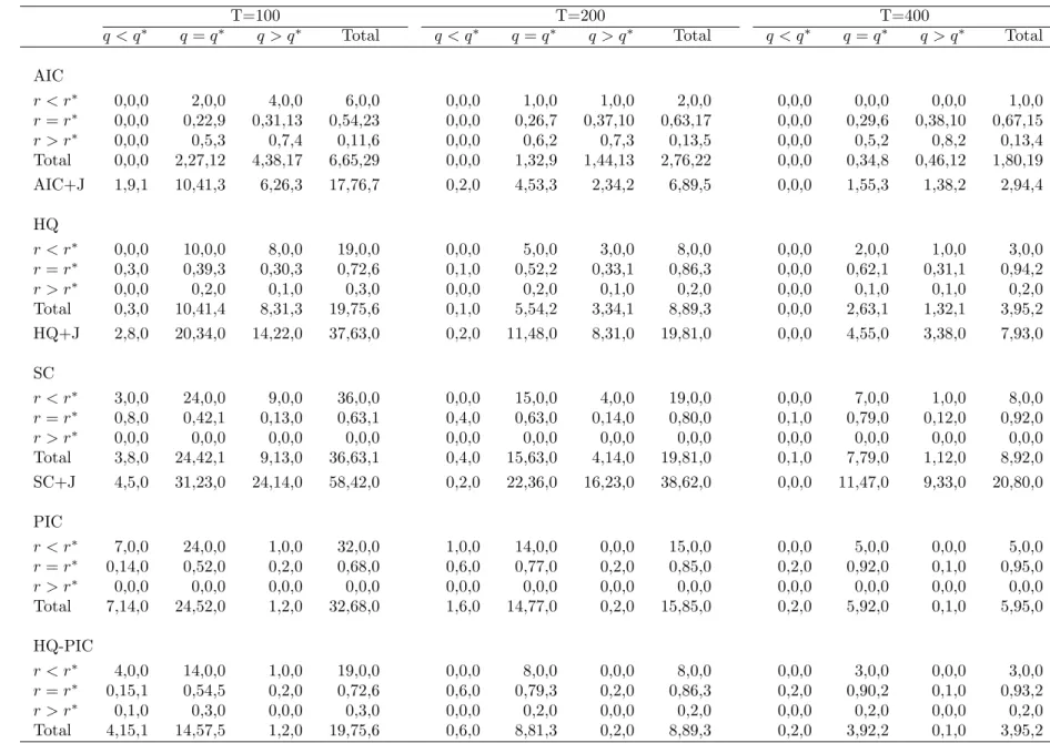
Simulation results are reported in “three-dimensional” frequency tables. The columns correspond to
the percentage of times the selected models had cointegrating rank smaller than the true rank (q < q∗),
equal to the true rank (q=q∗) and larger than the true rank (q > q∗). The rows correspond to similar
information about the rank of short-run dynamics r. Information about the lag-length is provided
within each cell, where the entry is disaggregated on the basis of p. The three numbers provided in
each cell, from left to right, correspond to percentages with lag lengths smaller than the true lag, equal
to the true lag and larger than true lag. The ‘Total’ column on the right margin of each table provides
information about marginal frequencies of p and r only. The row titled ‘Total’ on the bottom margin
of each table provides information about the marginal frequencies ofpand q only. Finally, the bottom
right cell provides marginal information about the lag-length choice only.
We report results of two sets of 100 DGPs. Table 1 summarises the model selection results for 100
DGPs that have one lag in differences with a short-run rank of one and cointegrating rank of two, i.e.,
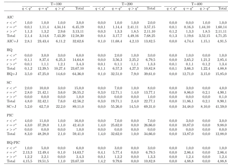
(p∗, r∗, q∗) = (1,1,2). Table 2 summarises the model selection results for 100 DGPs that have two lags
in differences with a short-run rank of one and cointegrating rank of one (p∗, r∗, q∗) = (2,1,1). These
two groups of DGPs are contrasting in the sense that the second group of DGPs have more severe
restrictions in comparison to the first one.
The first three panels of the tables correspond to all model selection based on the traditional model
selection criteria. The additional bottom row for each of these three panels provides information about
the lag-length and the cointegrating rank, when the lag-length is chosen using the simple version of
that model selection criterion and the cointegrating rank is chosen using the Johansen procedure,
and in particular the sequential trace test with 5% critical values that are adjusted for sample size.
Comparing the rows labelled ‘AIC+J’, ‘HQ+J’ and ‘SC+J’, we conclude that the inference about q
is not sensitive to whether the selected lag is correct or not. In Table 1 all three criteria choose the
correctq approximately 54%, 59% and 59% of the time for sample sizes 100, 200 and 400, respectively.
In Table 2 all three criteria choose the correct q approximately 70%, 82% and 82% of the time for
sample sizes 100, 200 and 400, respectively.
From the first three panels of Table 1 we can clearly see that traditional model selection criteria
are not appropriate for choosing p, qand r jointly, as expected from theory. The percentages of times
the correct model is chosen are only 22%, 26% and 29% with the AIC, 39%, 52% and 62% with HQ,
and 42%, 63% and 79% with SC, for sample sizes of 100, 200 and 400, respectively. Note that when
conclusion that is consistent with results in Vahid and Issler (2002).
The main reason for not being able to determine the triplet (p, r, q) correctly is the failure of these
criteria to choose the correct q. Ploberger and Phillips (2003) show that the correct penalty for free
parameters in the long-run parameter matrix is larger than the penalty considered by traditional model
selection criteria. According to this theory, all three criteria are expected to over-estimate q, and of
them SC is likely to appear relatively most successful because it assigns a larger penalty to all free
parameters, even though the penalty is still less than it should be for this design. This is exactly what
the simulations reveal.
The fourth panel of Table 1 includes results for the PIC. The percentages of times the correct model
is chosen increase to 52%, 77% and 92% for sample sizes of 100, 200 and 400, respectively. Comparing
the margins, it becomes clear that this increased success relative to HQ and SC is almost entirely due
to improved precision in the selection of q. The PIC chooses q correctly 76%, 91% and 97% of the
time for sample sizes 100, 200 and 400, respectively. Furthermore, for the selection of p and r only,
PIC does not improve upon HQ, a fact that we will exploit to propose a two-step procedure for model
selection with partially non-stationary time series.
Similar conclusions can be reached from the results for the (2,1,1) DGPs presented in Table 2.
We note that in this case, even though the PIC improves on HQ and SC in choosing the number of
cointegrating vectors, it does not improve on HQ or SC in choosing the exact model, because it severely
underestimates p. This echoes the findings of Vahid and Issler (2002) in the stationary case that the
Schwarz criterion (recall that the PIC penalty is of the same order as the Schwarz penalty in the
stationary case) severely underestimates the lag length in small samples in reduced rank VARs. They
re-visit some of the early studies that documented evidence in favour of the SC and conclude that the
results of those studies are artifacts of a very short lag length and a strong propagation mechanism in
the true DGP. The results of our (2,1,1) design and our other experiments with DGPs with longer lags
(not reported here) confirm that the only advantage of PIC is in the determination of the cointegrating
rank.
6.1.1 A two-step procedure for model selection
Our Monte-Carlo results show that the advantage of PIC over HQ and SC is in the determination of
the cointegrating rank. Indeed, HQ seems to have an advantage over PIC in selecting the correct p
and r in small samples. In addition, the calculation of PIC for the set of all reduced rank VECMs up
to a predetermined maximum lag length requires the coding and calculation of many high dimensional
matrices. Even after normalising the elements of the FIM, it is possible, as happened in our
unreliable. These facts motivated us to consider a two-step alternative to improve the model selection
task.
In the first step, the linear influence of yt−1 is removed from ∆yt and (∆yt−1, ...,∆yt−p), then
HQ(p, r), as defined in (7), is used to determinepand r. Then PIC is calculated for the chosen values
of p andr, for all q from 0 to K. This reduces the task to K+ 1 determinant calculations only.
The final panels in Tables 1 and 2 summarise the performance of this two-step procedure for the
two sets of DGPs we consider. In both tables we can see that the hybrid HQ-PIC procedure improves
on all other criteria in selecting the exact model. The improvement is a consequence of the advantage
of HQ in selecting p andr better, and PIC in selecting q better.
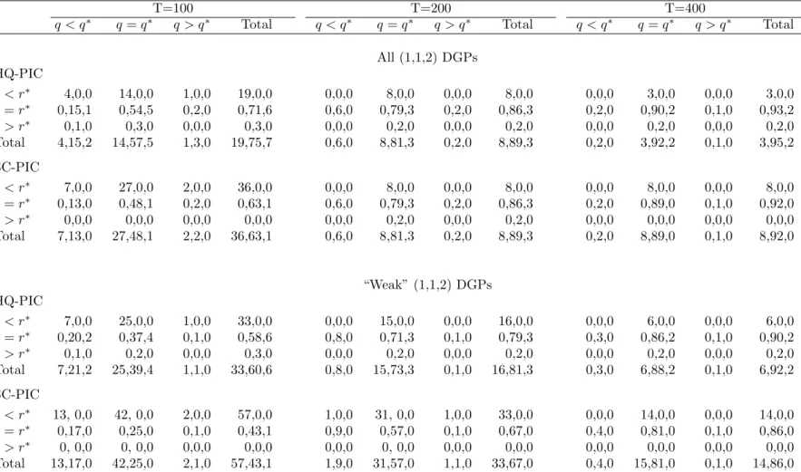
Table 3 provides this information for the hybrid HQ-PIC and SC-PIC for a (1,1,2) design and a
“weak” (as defined in Section 5) (1,1,2) design. The results highlight the advantage of HQ over SC in
the proposed two-stage model selection procedure, as the SC tends to under-parameterise the model.
Note that when the propagation mechanism is weak, the advantage of HQ-PIC over SC-PIC is further
accentuated. We found similar results for the (2,1,1) DGPs. Vahid and Issler (2002) show that this
tendency of the SC results in very poor forecasting performance in “weak” designs. In this setting we
also find that the advantage of the HQ-PIC over the SC-PIC in model selection translates to better
forecasting. We do not present these results here; however, they are available upon request.
Finally, the hybrid procedure results in over-parameterised models more often than PIC (see Tables
1 and 2). We examined whether this trade-off has any significant consequences for forecasting and found
that it does not. In all simulation settings, models selected by the hybrid procedure with HQ-PIC as
the model selection criteria forecast better than models selected by PIC. Again, we do not present
these results here, but they are also available upon request.
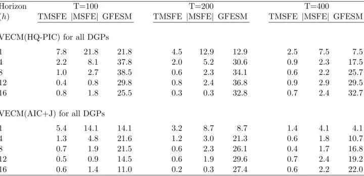
6.2 Forecasts
Recall that the forecasting results are expressed as the percentage improvement in forecast accuracy
measures of possibly rank reduced models over the unrestricted VAR model in levels selected by SC.
Also, note that the object of interest in this forecasting exercise is assumed to be the first difference of
variables.
We label the models chosen by the hybrid procedure proposed in the previous section and estimated
by the iterative process of Section 3 as VECM(HQ-PIC). We label the models estimated by the usual
Johansen method with AIC as the model section criterion for the lag order as VECM(AIC+J).
Table 4 presents the forecast accuracy improvements in a (1,1,2) setting. In terms of the trace
and determinant of the MSFE matrix, there is some improvement in forecasts over unrestricted VAR
With only 100 observations, GFESM worsens for horizons 8 and longer. This means that if the object
of interest was some combination of differences across different horizons (for example, the levels of all
variables or the levels of some variables and first differences of others), there may not have been any
improvement in the MSFE matrix. With 200 or more observations, all forecast accuracy measures show
some improvement, with the more substantial improvements being for the one-step-ahead forecasts.
Also note that the forecasts of the models selected by the hybrid procedure are almost always better
than those produced by the model chosen by the AIC plus Johansen method, which only pays attention
to lag-order and long-run restrictions.
Table 5 presents the forecast accuracy improvements in a (2,1,1) setting. This set of DGPs have
more severe rank reductions than the (1,1,2) DGPs, and, as a result, the models selected by the
hybrid procedure show more substantial improvements in forecasting accuracy over the VAR in levels,
in particular for smaller sample sizes. Forecasts produced by the hybrid procedure are also substantially
better than forecasts produced by the AIC+Johansen method, which does not incorporate short-run
rank restrictions. Note that although the AIC+Johansen forecasts are not as good as the HQ-PIC
forecasts, they are substantially better than the forecasts from unrestricted VARs at short horizons.
This is interesting in itself, and deserves further investigation because it is somewhat different from the
results of Engle and Yoo (1987), who report no gains for one-step-ahead forecasts. This difference may
be due to differences in the Monte Carlo design. Engle and Yoo’s results are based on a two variable
DGP with one cointegrating vector (only one restriction in the long-run parameter matrix) and no lag
differences, and the true lag length and the fact that there is no intercept in the DGP are assumed
known. We are currently investigating this.
7
Empirical example
The techniques discussed in this paper are applied to forecast Brazilian inflation, as measured by three
different types of consumer-price indices. The first is the consumer price index of the Brazilian
Inflation-Targeting Program. It is computed by IBGE, the official statistics bureau of the Brazilian government.
We label this index CPI-IBGE. The second is the consumer price index computed by Getulio Vargas
Foundation, a traditional private institution which has been computing several Brazilian price indices
since 1947. We label this index CPI-FGV. The third is the consumer price index computed by FIPE,
an institute of the Department of Economics of the University of S˜ao Paulo, labelled here as CPI-FIPE.
These three indices capture different aspects of Brazilian consumer-price inflation. First, they differ
in terms of geographical coverage. CPI-FGV collects prices in 12 different metropolitan areas in Brazil,
are not covered by CPI-FGV). Therefore, CPI-FGV and CPI-IBGE have a very similar coverage. On
the other hand, CPI-FIPE only collects prices in S˜ao Paulo – the largest city in Brazil – also covered
by the other two indices. Tracked consumption bundles are also different across indices. CPI-FGV
focuses on bundles of the representative consumer with income between 1 and 33 times minimum
wages. CPI-IBGE focuses on bundles of consumers with income between 1 and 40 times minimum
wages, while CPI-FIPE focuses on consumers with income between 1 and 20 times minimum wages.
Although all three indices measure consumer-price inflation in Brazil, Granger Causality tests
confirm the usefulness of conditioning on alternative indices to forecast any given index in the models
estimated here. We present this evidence below. Despite the existence of these forecasting gains,
one should expect a similar pattern for impulse-response functions across models, reflecting a similar
response of different price indices to shocks to the dynamic system. This last feature is simply a
reflection of the reduced-rank nature of the stationary models entertained here.
Data on CPI-FGV, CPI-IBGE, and CPI-FIPE are available on a monthly basis from 1994:9 to
2008:11, with a span of more than 14 years (171 observations). It was extracted from IPEADATA
– a public database with downloadable Brazilian data (http://www.ipeadata.gov.br/). We start our
analysis in 1994:9 because inflation levels prior to 1994:6 reached hyper-inflation proportions, something
that changed completely after a successful stabilization plan implemented in 1994:65.
In what follows we compare the forecasting performance of (i) the VAR in (log) levels, with
lag length chosen by the standard Schwarz criterion; (ii) the reduced rank model using standard
AIC for choosing the lag length and Johansen’s test for choosing the cointegrating rank, labelled
VECM(AIC+J); and (iii) the reduced rank model with rank and lag length chosen simultaneously
using the Hannan-Quinn criterion and cointegrating rank chosen using PIC, estimated by the iterative
process of Section 3, labelled VECM(HQ-PIC).
For all three models, the applicable choices ofp, r, and q use data from 1994:9 through 2004:12.
These choices are kept fixed for the forecasting exercise. For all three models, we compute their
h = 1, . . . ,16−step ahead forecasts, comprising a total of 32 balanced forecasts, which are then con-fronted with their respective realizations. This is performed from 2005:1 through 2008:11 – the
forecast-ing period, with 47 observations. All models are recursively re-estimated in the forecastforecast-ing period. All
forecasts comparisons are made in first differences of the logs of CPI-FGV, CPI-IBGE, and CPI-FIPE.
The choice of the lag length of the VAR in (log) levels for CPI-FGV, CPI-IBGE, and CPI-FIPE,
using the Schwarz criterion, was 2 lags, i.e., p = 1. All other standard criteria chose the same lag
length in this case. For the VECM(AIC+J), AIC chosep= 1, while Johansen’s test choseq= 1 at 5%
5
significance, regardless of whether one uses the trace or the λmax statistic. For the estimation sample
period from 1995:1 through 2004:12, the cointegrating vector found was:
log(CPI-FGVt) + 0.83×log(CPI-FIPEt)−1.70×log(CPI-IBGEt).
For the VECM(HQ-PIC), the iterative procedure described in Section 3 chose a reduced rank model
withp= 1,r = 2, andq = 0. This choice is consistent with direct testing for reduced-rank restrictions.
For example, taking the estimation sample period from 1995:1 through 2004:12, the common-cycle test
yields a smallest squared canonical correlation of 0.01, which is not significantly different from zero –
a p-value of 0.19191. This shows the existence of one co-feature vector (r= 2):
∆ log(CPI-FIPEt)−1.64×∆ log(CPI-IBGEt) + 0.50×∆ log(CPI-FGVt). (12)
The correlogram of this combination resembles that of a white-noise process.
In all stationary models considered here, it is clear that conditioning on information from other price
indices helps predict any given index. For example, all three cointegrating vectors are significant at the
1% level in all three VECM equations. For the reduced-rank model, ∆ log(CPI-IBGEt−1) is significant
in ∆ log(CPI-FGVt)’s equation, which helps predicting all the variables in the system through the
pseudo-structural relationship in (12).
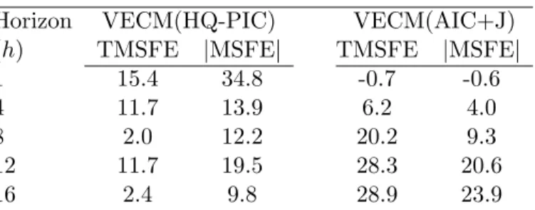
Table 6 presents the percentage improvement in forecast accuracy measures for the reduced rank
models over the unrestricted VAR model in (log) levels. We focus on the TMSFE and|MSFE|.6 When we consider the one-step ahead forecasts of the VECM(HQ-PIC) model, there is a percentage gain of
15.4% and 34.8% in the TMSFE and |MSFE|respectively over the VAR, whereas the performance of the VECM(AIC+J) is worse than VAR by 0.6% and 0.7% respectively. This makes the
VECM(HQ-PIC) model better than the VECM(AIC+J) forecasting one-step ahead by 16% and 35.5% respectively.
Results for 4-steps ahead are similar, although gains are not as much.
For horizons higher or equal to 8-steps ahead, VECM(HQ-PIC) and VECM(AIC+J) models both
forecast better than the unrestricted VAR, but VECM(AIC+J) produces substantially better forecasts
than the VECM(HQ-PIC). Given thatp= 1 in both models, this has to be the consequence of AIC+J
choosingq = 1 and HQ-PIC choosingq = 0 in this example. Withq= 1, long horizon forecasts of the
log-levels will be close to collinear, something the VECM(AIC+J) imposes but the VECM(HQ-PIC)
model does not. Collinearity of long-run forecasts of log-levels in this example is appealing because
these variables are consumer price indices with a large overlap in their construction. However, imposing
q = 1 has detrimental consequences for one month ahead and one quarter ahead forecasts of inflation,
6
which are objects of considerable importance. This trade-off between short and long run forecasts
motivates the possibility of using different models to forecast Brazilian inflation at different horizons,
which is an old but important topic in the forecasting literature but is beyond the scope of the present
paper.
8
Conclusion
Motivated by the results of Vahid and Issler (2002) on the success of the Hannan-Quinn criterion in
selecting the lag length and rank in stationary VARs, and the results of Ploberger and Phillips (2003)
and Chao and Phillips (1999) on the generalisation of Rissanen’s theorem to trending time series
and the success of PIC in selecting the cointegrating rank in VARs, we propose a combined HQ-PIC
procedure for the simultaneous choice of the lag-length and the ranks of the short-run and long-run
parameter matrices in a VECM. Our simulations show that this procedure is capable of selecting the
correct model more often than other alternatives such as pure PIC or SC.
In this paper we also present forecasting results that show that models selected using this hybrid
procedure produce better forecasts than unrestricted VARs selected by the Schwarz criterion and
cointegrated VAR models whose lag length is chosen by the AIC and whose cointegrating rank is
determined by the Johansen procedure. We have chosen these two alternatives for forecast comparisons
because we believe that these are the model selection strategies that are most often used in the empirical
literature. However, we have considered several other alternative model selection strategies and the
results are qualitatively the same: the hybrid HQ-PIC procedure leads to models that generally forecast
better than models selected using other procedures.
A conclusion we would like to highlight is the importance of short-run restrictions for forecasting.
We believe that there has been much emphasis in the literature on the effect of long-run cointegrating
restrictions on forecasting. Given that long-run restrictions involve the rank of only one of the
param-eter matrices of a VECM, and that inference on this matrix is difficult because it involves inference
about stochastic trends in variables, it is puzzling that the forecasting literature has paid so much
attention to cointegrating restrictions and relatively little attention to lag-order and short-run
restric-tions in a VECM. The present paper fills this gap and highlights the fact that the lag-order and the
rank of short-run parameter matrices are as important for forecasting as cointegrating restrictions. Our
hybrid model selection procedure and the accompanying simple iterative procedure for the estimation
of a VECM with long-run and short-run restrictions provide a reliable methodology for developing
multivariate autoregressive models that are useful for forecasting.
real life data generating processes is an empirical question. Macroeconomic models in which trends
and cycles in all variables are generated by a small number of dynamic factors fit in this category. Also,
empirical papers that study either regions of the same country or similar countries in the same region
often find these kinds of long-run and short-run restrictions. In the empirical example in this paper,
we look at jointly forecasting three different measures of consumer price inflation in Brazil, and we
find that reduced rank models chosen by the methods considered in this paper produce better forecasts
than unrestricted VARs. We also observe that there is some scope for using different reduced rank
models for forecasting Brazilian inflation at different horizons, a possibility that is not directly related
to the scope of the current paper but can be quite important for users of these forecasts and deserves
further research.
References
Ahn, S. K. and G. C. Reinsel (1988) Nested reduced-rank autoregressive models for multiple time
series,Journal of the American Statistical Association,83, 849–856.
Anderson, T. (1951) Estimating linear restrictions on regression coefficients for multivariate normal
distributions,Annals of Mathematical Statistics,22, 327–351.
Athanasopoulos, G. and F. Vahid (2008) VARMA versus VAR for macroeconomic forecasting,Journal
of Business and Economic Statistics,26, 237–252.
Centoni, M., G. Cubbada and A. Hecq (2007) Common shocks, common dynamics and the international
business cycle,Economic Modelling,24, 149–166.
Chao, J. and P. Phillips (1999) Model selection in partially nonstationary vector autoregressive
pro-cesses with reduced rank structure,Journal of Econometrics,91, 227–271.
Christoffersen, P. and F. Diebold (1998) Cointegration and long-horizon forecasting,Journal of
Busi-ness and Economic Statistics,16, 450–458.
Clements, M. P. and D. F. Hendry (1993) On the limitations of comparing mean squared forecast
errors (with discussions),Journal of Forecasting,12, 617–637.
Clements, M. P. and D. F. Hendry (1995) Forecasting in cointegrated systems, Journal of Applied
Econometrics,10, 127–146.
Engle, R. F. and S. Yoo (1987) Forecasting and testing in cointegrated systems,Journal of
Gonzalo, J. and J.-Y. Pitarakis (1999) Dimensionality effect in cointegration tests, in Cointegration,
Causality and Forecasting, eds. R. F. Engle and H. White, A Festschrift in Honour of Clive W. J.
Granger, New York: Oxford University Press, pp. 212-229.
Gourieroux, C. and I. Peaucelle (1992) Series codependantes application a l’hypothese de parite du
pouvoir d’achat,Revue d’Analyse Economique,68, 283–304.
Hecq, A., F. Palm and J.-P. Urbain (2006) Common cyclical features analysis in VAR models with
cointegration,Journal of Econometrics,132, 117–141.
Hoffman, D. and R. Rasche (1996) Assessing forecast performance in a cointegrated system, Journal
of Applied Econometrics,11, 495–517.
Johansen, S. (1988) Statistical analysis of cointegrating vectors, Journal of Economic Dynamics and
Control,12, 231–254.
Johansen, S. (1991) Estimation and hypothesis testing of cointegration vectors in gaussian vector
autoregressive models,Econometrica,59, 1551–1580.
Johansen, S. (2002) A small sample correction of the test for cointegrating rank in the vector
autore-gressive model,Journal of Econometrics,70, 195–221.
Lin, J. L. and R. S. Tsay (1996) Cointegration constraints and forecasting: An empirical examination,
Journal of Applied Econometrics,11, 519–538.
L¨utkepohl, H. (1985) Comparison of criteria for estimating the order of a vector autoregressive process,
Journal of Time Series Analysis,9, 35–52.
L¨utkepohl, H. (1993) Introduction to multiple time series analysis, Springer-Verlag, Berlin-Heidelberg,
2nd ed.
Magnus, J. R. and H. Neudecker (1988) Matrix differential calculus with applications in statistics and
econometrics, New York: John Wiley and Sons.
Phillips, P. and W. Ploberger (1996) An asymptitic theory of Bayesian inference for time series,
Econo-metrica,64, 381–413.
Phillips, P. C. B. (1996) Econometric model determination, Econometrica,64, 763–812.
Phillips, P. C. B. and B. Hansen (1990) Statistical inference in instrumental variables regression with
Phillips, P. C. B. and M. Loretan (1991) Estimating long-run economic equilibria,Review of Economic
Studies,58, 407–436.
Ploberger, W. and P. C. B. Phillips (2003) Empirical limits for time series econometric models,
Econo-metrica,71, 627–673.
Poskitt, D. S. (1987) Precision, complexity and bayesian model determination, Journal of the Royal
Statistical Society B,49, 199–208.
Rissanen, J. (1987) Stochastic complexity,Journal of the Royal Statistical Society B,49, 223–239. Saikkonen, P. (1992) Estimation and testing of cointegrated systems by an autoregressive
approxima-tion,Econometric Theory,8, 1–27.
Silverstovs, B., T. Engsted and N. Haldrup (2004) Long-run forecasting in multicointegrated systems,
Journal of Forecasting,23, 315–335.
Vahid, F. and R. F. Engle (1993) Common trends and common cycles,Journal of Applied Econometrics,
8, 341–360.
Vahid, F. and J. V. Issler (2002) The importance of common cyclical features in VAR analysis: A
Monte-Carlo study,Journal of Econometrics,109, 341–363.
Velu, R., G. Reinsel and D. Wickern (1986) Reduced rank models for multiple time series,Biometrika,
73, 105–118.
Wallace, C. (2005)Statistical and inductive inference by minimum message length, Berlin: Springer.
Wallace, C. and P. Freeman (1987) Estimation and inference by compact coding,Journal of the Royal
Statistical Society B,49, 240–265.
A
Proof of Lemma 1
Subtracting yt−1 from both sides of the first equation in (1) and adding an subtracting βy2t−1 from
the right side of the same equation leads to
∆y1t = −(y1t−1−βy2t−1) +β∆y2t+u1t
which, after substitutingu2t for ∆y2t on the first line, can be written as
∆yt=−
Iq −β
0 0
yt−1+vt (13)
where
vt=
Iq β
0 IK−q
ut.
Since vtis a full rank linear transformation of vectorut, it will also be a VAR of order pand rank less
than or equal to r, i.e.,
vt=F1vt−1+F2vt−2+· · ·+Fpvt−p+ηt,
where Fi =
Iq β
0 IK−q
Bi
Iq β
0 IK−q −1
fori= 1, ..., p, and ηt =
Iq β
0 IK−q
εt.The matrix
F1 F2 ... Fp has rank less than or equal to r because it is the product of B1 B2 ... Bp
and full rank matrices. Consider the characteristic polynomial of the vector autoregression that
char-acterises the dynamics of vt:
G(L) =IK−F1L−F2L2− · · · −FpLp.
Using the identity G(L) =G(1) +G∗(L) (I
K−L),we can write this polynomial as:
G(L) = IK−F1−F2− · · · −Fp+ p X i=1 Fi+ p X i=2
FiL+· · ·+
p X
i=p−1
FiLp−2+FpLp−1
(IK−L).
Pre-multiplying both sides of (13) by G(L), using the G(1) +G∗(L) (I
K−L) formulation of G(L)
only when we apply it to theyt−1 term, and noting that G(L)vt=ηt,we obtain
G(L) ∆yt = −(IK−F1−F2− · · · −Fp)
Iq −β
0 0
yt−1
− p X i=1 Fi+ p X i=2
FiL+· · ·+
p X
i=p−1
FiLp−2+FpLp−1
Iq −β
0 0
∆yt−1+ηt.
Expanding the left side of the equation, taking all lagged terms to the right, and denoting the first q
columns of −(IK−F1−F2− · · · −Fp) byγ, we obtain
∆yt=γ Iq −β
yt−1+
p X
j=1
Fj− p X
i=j Fi
Iq −β
0 0
∆yt−j+ηt.
Defining
Γj =Fj− p X
i=j Fi
Iq −β
0 0
for j = 1, ..., p, we note that each Γj is the result of elementary column operations
on the matrix F=
F1 F2 ... Fp
,and therefore they cannot have rank larger than the rank of
F.Moreover, all vectors in the null-space ofF would also lie in the null-space of
Γ1 Γ2 ... Γp
.
Therefore, rank
Γ1 Γ2 ... Γp
≤rank(F)≤r.
B
The Fisher information matrix of the reduced rank VECM
Assuming that the first observation in the sample is labelled observation −p+ 1 and that the sample containsT +p observations, we write theK-variable reduced rank VECM
∆yt=γ′ Iq β′
yt−1+
Ir C′
[D1∆yt−1+D2∆yt−2+· · ·+Dp∆yt−p] +µ+et,
or in stacked form
∆Y =Y−1
Iq
β
γ+W D Ir C
+ιTµ′+E,
where
∆Y T×K =
∆y1′
.. . ∆yT′
, Y−1 T×K
=
y0′
.. .
yT′ −1
, TE
×K =
e′1
.. .
e′T
W
T×Kp = ∆Y−1 · · · ∆Y−p
=
∆y′
0 · · · ∆y−′ p+1 ..
. ... ... ∆y′T−1 · · · ∆y′T−p
D Kp×r =
D′ 1 .. .
Dp′
,
and ιT is a T ×1 vector of ones. When et are N(0,Ω) and serially uncorrelated, the log-likelihood function, conditional on the first p observations being known, is:
lnl(θ, ω) = −KT
2 ln (2π)−
T
2 ln|Ω| − 1 2
T X
t=1
e′tΩ−1et
= −KT
2 ln (2π)−
T
2 ln|Ω| − 1
2tr EΩ −1E′
, where θ=
vec(β)
vec(γ)
vec(D)
vec(C)
is a (K−q)q+Kq+Kpr+r(K−r)+Kmatrix of mean parameters, andω=vech(Ω) is aK(K+ 1)/2 vector of unique elements of the variance matrix. The differential of the log-likelihood is (see Magnus
and Neudecker, 1988)
dlnl(θ, ω) = −T
2trΩ
−1dΩ + 1 2tr Ω
−1dΩΩ−1E′E
−1
2tr Ω
−1E′dE
−1
2tr Ω
−1dE′E
= 1
2tr Ω
−1 E′E−TΩ
Ω−1dΩ
−tr Ω−1E′dE ,
and the second differential is:
d2lnl(θ, ω) = tr dΩ−1 E′E−TΩ
Ω−1dΩ
+1 2tr Ω
−1 2E′dE−T dΩ
Ω−1dΩ
−tr dΩ−1E′dE
−tr Ω−1dE′dE .
Since we eventually want to evaluate the Fisher information matrix at the maximum likelihood
esti-mator, and at the maximum likelihood estimator ˆE′Eˆ−TΩ = 0ˆ ,and also ˆΩ−1Eˆ′dE/dθ= 0 (these are apparent from the first differentials), we can delete these terms from the second differential, and use
tr(AB) =vec(A′)′vec(B) to obtain
d2lnl(θ, ω) = −T
2tr Ω
−1dΩΩ−1dΩ
−tr Ω−1dE′dE
= −T
2 (dω) ′D′
K Ω−1⊗Ω−1
DKdω−(vec(dE))′ Ω−1⊗IT
vec(dE),
where DK is the “duplication matrix”. From the model, we can see that
dE=−Y−1
0
dβ
γ−Y−1
Iq
β
dγ−W dD Ir C
−W D 0 dC
−ιTdµ′,
and therefore
vec(dE) =−
γ′⊗Y−(2)1 IK⊗Y−1
Iq β Ir C′ ⊗W 0
IK−r
⊗W D IK⊗ιT