❊♥s❛✐♦s ❊❝♦♥ô♠✐❝♦s
❊s❝♦❧❛ ❞❡
Pós✲●r❛❞✉❛çã♦
❡♠ ❊❝♦♥♦♠✐❛
❞❛ ❋✉♥❞❛çã♦
●❡t✉❧✐♦ ❱❛r❣❛s
◆◦ ✼✵✹ ■❙❙◆ ✵✶✵✹✲✽✾✶✵
▼♦❞❡❧ s❡❧❡❝t✐♦♥✱ ❡st✐♠❛t✐♦♥ ❛♥❞ ❢♦r❡❝❛st✐♥❣
✐♥ ❱❆❘ ♠♦❞❡❧s ✇✐t❤ s❤♦rt✲r✉♥ ❛♥❞ ❧♦♥❣✲r✉♥
r❡str✐❝t✐♦♥s
●❡♦r❣❡ ❆t❤❛♥❛s♦♣♦✉❧♦s✱ ❖s♠❛♥✐ ❚❡✐①❡✐r❛ ❞❡ ❈❛r✈❛❧❤♦ ●✉✐❧❧é♥✱ ❏♦ã♦ ❱✐❝✲ t♦r ■ss❧❡r✱ ❋❛rs❤✐❞ ❱❛❤✐❞
❖s ❛rt✐❣♦s ♣✉❜❧✐❝❛❞♦s sã♦ ❞❡ ✐♥t❡✐r❛ r❡s♣♦♥s❛❜✐❧✐❞❛❞❡ ❞❡ s❡✉s ❛✉t♦r❡s✳ ❆s
♦♣✐♥✐õ❡s ♥❡❧❡s ❡♠✐t✐❞❛s ♥ã♦ ❡①♣r✐♠❡♠✱ ♥❡❝❡ss❛r✐❛♠❡♥t❡✱ ♦ ♣♦♥t♦ ❞❡ ✈✐st❛ ❞❛
❋✉♥❞❛çã♦ ●❡t✉❧✐♦ ❱❛r❣❛s✳
❊❙❈❖▲❆ ❉❊ PÓ❙✲●❘❆❉❯❆➬➹❖ ❊▼ ❊❈❖◆❖▼■❆ ❉✐r❡t♦r ●❡r❛❧✿ ❘❡♥❛t♦ ❋r❛❣❡❧❧✐ ❈❛r❞♦s♦
❉✐r❡t♦r ❞❡ ❊♥s✐♥♦✿ ▲✉✐s ❍❡♥r✐q✉❡ ❇❡rt♦❧✐♥♦ ❇r❛✐❞♦ ❉✐r❡t♦r ❞❡ P❡sq✉✐s❛✿ ❏♦ã♦ ❱✐❝t♦r ■ss❧❡r
❉✐r❡t♦r ❞❡ P✉❜❧✐❝❛çõ❡s ❈✐❡♥tí✜❝❛s✿ ❘✐❝❛r❞♦ ❞❡ ❖❧✐✈❡✐r❛ ❈❛✈❛❧❝❛♥t✐
❆t❤❛♥❛s♦♣♦✉❧♦s✱ ●❡♦r❣❡
▼♦❞❡❧ s❡❧❡❝t✐♦♥✱ ❡st✐♠❛t✐♦♥ ❛♥❞ ❢♦r❡❝❛st✐♥❣ ✐♥ ❱❆❘ ♠♦❞❡❧s ✇✐t❤ s❤♦rt✲r✉♥ ❛♥❞ ❧♦♥❣✲r✉♥ r❡str✐❝t✐♦♥s✴
●❡♦r❣❡ ❆t❤❛♥❛s♦♣♦✉❧♦s✱ ❖s♠❛♥✐ ❚❡✐①❡✐r❛ ❞❡ ❈❛r✈❛❧❤♦ ●✉✐❧❧é♥✱ ❏♦ã♦ ❱✐❝t♦r ■ss❧❡r✱ ❋❛rs❤✐❞ ❱❛❤✐❞ ✕ ❘✐♦ ❞❡ ❏❛♥❡✐r♦ ✿ ❋●❱✱❊P●❊✱ ✷✵✶✵
✭❊♥s❛✐♦s ❊❝♦♥ô♠✐❝♦s❀ ✼✵✹✮ ■♥❝❧✉✐ ❜✐❜❧✐♦❣r❛❢✐❛✳
Model selection, estimation and forecasting in VAR models with
short-run and long-run restrictions
George Athanasopoulos
Department of Econometrics and Business Statistics Monash University, Clayton, Victoria 3800
Australia
Osmani Teixeira de Carvalho Guillén Banco Central do Brasil and Ibmec-RJ
Av. Presidente Vargas, 730 - Centro Rio de Janeiro, RJ 20071-001
Brazil
João Victor Issler
Graduate School of Economics – EPGE Getulio Vargas Foundation Praia de Botafogo 190 s. 1111
Rio de Janeiro, RJ 22253-900 Brazil
Farshid Vahid
Department of Econometrics and Business Statistics Monash University, Clayton, Victoria 3800
Australia
Mar 15, 2010
Abstract
We study the joint determination of the lag length, the dimension of the cointegrating space and the rank of the matrix of short-run parameters of a vector autoregressive (VAR) model using model selection criteria. We consider model selection criteria which have data-dependent penalties as well as the traditional ones. We suggest a new two-step model selection procedure which is a hybrid of traditional criteria and criteria with data-dependant penalties and we prove its consistency. Our Monte Carlo simulations measure the improvements in forecasting accuracy that can arise from the joint determination of lag-length and rank using our proposed procedure, relative to an unrestricted VAR or a cointegrated VAR estimated by the commonly used procedure of selecting the lag-length only and then testing for cointegration. Two empirical applications forecasting Brazilian in‡ation and U.S. macroeconomic aggregates growth rates respectively show the usefulness of the model-selection strategy proposed here. The gains in di¤erent measures of forecasting accuracy are substantial, especially for short horizons.
Keywords: Reduced rank models, model selection criteria, forecasting accuracy. JEL Classi…cation: C32, C53.
1
Introduction
There is a large body of literature on the e¤ect of cointegration on forecasting. Engle and Yoo (1987)
compare the forecasts generated from an estimated vector error correction model (VECM) assuming
that the lag order and the cointegrating rank are known, with those from an estimated VAR in levels
with the correct lag. They …nd out that the VECM only produces forecasts with smaller mean squared
forecast errors (MSFE) in the long-run. Clements and Hendry (1995) note that Engle and Yoo’s
conclusion is not robust if the object of interest is di¤erences rather than levels, and use this observation
to motivate their alternative measures for comparing multivariate forecasts. Ho¤man and Rasche
(1996) con…rm Clements and Hendry’s observation using a real data set. Christo¤ersen and Diebold
(1998) also use Engle and Yoo’s setup, but argue against using a VAR in levels as a benchmark on the
grounds that the VAR in levels not only does not impose cointegration, it does not impose any unit
roots either. Instead, they compare the forecasts of a correctly speci…ed VECM with forecasts from
correctly speci…ed univariate models, and …nd no advantage in MSFE for the VECM. They use this
result as a motivation to suggest an alternative way of evaluating forecasts of a cointegrated system.
Silverstovs et al. (2004) extend Christo¤ersen and Diebold’s results to multicointegrated systems. Since
the afore-mentioned papers condition on the correct speci…cation of the lag length and cointegrating
rank, they cannot provide an answer as to whether we should examine the cointegrating rank of a
system in multivariate forecasting if we do not have any a priori reason to assume a certain form of
cointegration.
Lin and Tsay (1996) examine the e¤ect on forecasting of the mis-speci…cation of the cointegrating
rank. They determine the lag order using the AIC, and compare the forecasting performance of
estimated models under all possible numbers of cointegrating vectors (0 to 4) in a four-variable system.
They observe that, keeping the lag order constant, the model with the correct number of cointegrating
vectors achieves a lower MSFE for long-run forecasts, especially relative to a model that over-speci…es
the cointegrating rank. Although Lin and Tsay do not assume the correct speci…cation of the lag
length, their study also does not address the uncertainty surrounding the number of cointegrating
vectors in a way that can lead to a modelling strategy for forecasting possibly cointegrated variables.
Indeed, the results of their example with real data, in which they determine the cointegrating rank
using a sequence of hypothesis tests, do not accord with their simulation results.
At the same time, there is an increasing amount of evidence of the advantage of considering rank
restrictions for short-term forecasting in stationary VAR (and VARMA) models (see, for example, Ahn
and Reinsel 1988, Vahid and Issler 2002, Athanasopoulos and Vahid 2008). One feature of these papers
dimension of the most parsimonious state vector that can represent the dynamics of a system. Here,
we add the cointegrating rank to the menu of unknowns and evaluate model selection criteria that
determine all of these unknowns simultaneously. Our goal is to determine a modelling strategy that is
useful for multivariate forecasting.
There are other papers in the literature that evaluate the performance of model selection criteria
for determining lag-length and cointegrating rank, but they do not evaluate the forecast performance
of the resulting models. Gonzalo and Pitarakis (1999) show that in large systems the usual model
selection procedures may severely underestimate the cointegrating rank. Chao and Phillips (1999)
show that the posterior information criterion (PIC) performs well in choosing the lag-length and the
cointegrating rank simultaneously.
In this paper we evaluate the performance of model selection criteria in the simultaneous choice
of the lag-length p, the rank of the cointegrating space q, and the rank of other parameter matrices r
in a vector error correction model. We suggest a hybrid model selection strategy that selects p and r
using a traditional model selection criterion, and then chooses q based on PIC. We then evaluate the
forecasting performance of models selected using these criteria.
Our simulations cover the three issues of model building, estimation, and forecasting. We examine
the performances of model selection criteria that choose p; r and q simultaneously (IC(p; r; q)), and
compare their performances with a procedure that choosespusing a standard model selection criterion
(IC(p)) and determines the cointegrating rank using a sequence of likelihood ratio tests proposed by
Johansen (1988). We provide a comparison of the forecasting accuracy of …tted VARs when only
coin-tegration restrictions are imposed, when coincoin-tegration and short-run restrictions are jointly imposed,
and when neither are imposed. These comparisons take into account the possibility of model
misspec-i…cation in choosing the lag length of the VAR, the number of cointegrating vectors, and the rank of
other parameter matrices. In order to estimate the parameters of a model with both long-run and
short-run restrictions, we propose a simple iterative procedure similar to the one proposed by Centoni
et al. (2007).
It is very di¢cult to claim that any result found in a Monte Carlo study is general, especially in
multivariate time series. There are examples in the VAR literature of Monte Carlo designs which led
to all model selection criteria overestimating the true lag in small samples, therefore leading to the
conclusion that the Schwarz criterion is the most accurate. The most important feature of these designs
is that they have a strong propagation mechanism.1 There are other designs with weak propagation
mechanisms that result in all selection criteria underestimating the true lag and leading to the
conclu-1Our measure of the strength of the propagation mechanism is proportional to the trace of the product of the variance
sion that AIC’s asymptotic bias in overestimating the true lag may actually be useful in …nite samples
(see Vahid and Issler 2002, for references). We pay particular attention to the design of the Monte
Carlo to make sure that we cover a wide range of data generating processes in terms of the strength of
their propagation mechanisms.
The outline of the paper is as follows. In Section 2 we study …nite VARs with long-run and
short-run restrictions and motivate their empirical relevance. In Section 3, we outline an iterative procedure
for computing the maximum likelihood estimates of parameters of a VECM with short-run restrictions.
We provide an overview of model selection criteria in Section 4, and in particular we discuss model
selection criteria with data dependent penalty functions. Section 5 describes our Monte Carlo design.
Section 6 presents the simulation results and Section 8 concludes.
2
VAR models with long-run and short-run common factors
We start from the triangular representation of a cointegrated system used extensively in the
coin-tegration literature (some early examples are Phillips and Hansen 1990, Phillips and Loretan 1991,
Saikkonen 1992). We assume that the K-dimensional time series
yt= y1t
y2t ; t= 1; :::; T
wherey1t isq 1 (implying thaty2tis (K q) 1) is generated from:
y1t = y2t+u1t (1)
y2t = u2t
where is aq (K q) matrix of parameters, and
ut= u1t u2t
is a strictly stationary process with mean zero and positive de…nite covariance matrix. This is a data
generating process (DGP) of a system of K cointegrated I(1) variables with q cointegrating vectors,
also referred to as a system ofK I(1) variables withK qcommon stochastic trends (some researchers
also refer to this as a system ofK variables withK q unit roots, which can be ambiguous if used out
of context, and we therefore do not use it here).2 The extra feature that we add to this fairly general
DGP is that ut is generated from a VAR of …nite order p and rankr (< K).
2While in theory every linear system ofK cointegrated I(1) variables withq cointegrating vectors can be represented
in this way, in practice the decision on how to partitionK-variables intoy1tandy2tis not trivial, becausey1tare variables
In empirical applications, the …nite VAR(p) assumption is routine. This is in contrast to the
theoretical literature on testing for cointegration, in which ut is assumed to be an in…nite VAR, and
a …nite VAR(p) is used as an approximation (e.g. Saikkonen 1992). Here, our emphasis is on building
multivariate forecasting models rather than hypothesis testing. The …nite VAR assumption is also
routine when the objective is studying the maximum likelihood estimator of the cointegrating vectors,
as in Johansen (1988).
The reduced rank assumption is considered for the following reasons. Firstly, this assumption
means that all serial dependence in the K-dimensional vector time series ut can be characterised by
only r < K serially dependent indices. This is a feature of most macroeconomic models, in which
the short-run dynamics of the variables around their steady states are generated by a small number
of serially correlated demand or supply shifters. Secondly, this assumption implies that there are
K r linear combinations of ut that are white noise. Gourieroux and Peaucelle (1992) call such time
series “codependent,” and interpret the white noise combinations as equilibrium combinations among
stationary variables. This is justi…ed on the grounds that, although each variable has some persistence,
the white noise combinations have no persistence at all. For instance, if an optimal control problem
implies that the policy instrument should react to the current values of the target variables, then it is
likely that there will be such a linear relationship between the observed variables up to a measurement
noise. Finally, many papers in multivariate time series literature provide evidence of the usefulness of
reduced rank VARs for forecasting (see, for example, Velu et al. 1986, Ahn and Reinsel 1988). Recently,
Vahid and Issler (2002) have shown that failing to allow for the possibility of reduced rank structure
can lead to developing seriously misspeci…ed vector autoregressive models that produce bad forecasts.
The dynamic equation for ut is therefore given by (all intercepts are suppressed to simplify the
notation)
ut=B1ut 1+B2ut 2+ +Bput p+"t (2)
whereB1; B2; :::; BpareK Kmatrices withrank B1 B2 ::: Bp =r, and"tis an i.i.d. sequence
with mean zero and positive de…nite variance-covariance matrix and …nite fourth moments. Note that
the rank condition implies that each Bi has rank at most r, and the intersection of the null-spaces
of all Bi is a subspace of dimension K r. The following lemma derives the vector error correction
representation of this data generating process.
Lemma 1 The data generating process given by equations (1) and (2) has a reduced rank vector error
correction representation of the type
yt= Iq yt 1+ 1 yt 1+ 2 yt 2+ + p yt p+ t; (3)
Proof. Refer to the working paper version of the current paper.
This lemma shows that the triangular DGP (1) under the assumption that the dynamics of its
stationary component (i.e. ut) can be characterised by a small number of common factors, is equivalent
to a VECM in which the coe¢cient matrices of lagged di¤erences have reduced rank and their left
null-spaces overlap. Hecq et al. (2006) call such a structure a VECM with weak serial correlation common
features (WSCCF).
We should note that the triangular structure (1) implies K q common Beveridge-Nelson (BN)
trends, but the reduced rank structure assumed for ut does not imply that deviations from the BN
trends (usually refereed to as BN cycles) can be characterised as linear combinations of r common
factors. Vahid and Engle (1993) show that a DGP with common BN trends and cycles is a special
case of the above under some additional restrictions and therefore a stricter form of comevement. Hecq
et al. (2006) show that the uncertainty in determining the rank of the cointegrating space can adversely
a¤ect inference on common cycles, and they conclude that testing for weak common serial correlation
features is a more accurate means of uncovering short-run restrictions in vector error correction models.
Our objective is to come up with a model development methodology that allows for cointegration
and weak serial correlation common features. For stationary time series, Vahid and Issler (2002) show
that allowing for reduced rank models is bene…cial for forecasting. For partially non-stationary time
series, there is an added dimension of cointegration. Here, we examine the joint bene…ts of cointegration
and short-run rank restrictions for forecasting partially non-stationary time series.
3
Estimation of VARs with short-run and long-run restrictions
The maximum likelihood estimation of the parameters of a VAR written in error-correction form
yt= yt 1+ 1 yt 1+ 2 yt 2+ + p yt p+ t (4)
under the long-run restriction that the rank of is q, the short-run restriction that rank of
[ 1 2 ::: p ] is r and the assumption of normality, is possible via a simple iterative procedure
that uses the general principle of the estimation of reduced rank regression models Anderson (1951).
Noting that the above model can be written as
yt = 0yt 1+C[D1 yt 1+D2 yt 2+ +Dp yt p] + t; (5)
where is aK q matrix of rankqandC is aK r matrix of rankr, one realises that if was known,
CandDi; i= 1; : : : ; p, could be estimated using a reduced rank regression of yton yt 1; ; yt p
after partialling out 0
using a reduced rank regression of yt on yt 1 after controlling forPpi=1Di yt i. This points to an
easy iterative procedure for computing maximum likelihood estimates for all parameters.
Step 0. Estimate [ ^D1;D^2; : : : ;Dp^ ] from a reduced rank regression of yt on ( yt 1; :::; yt p)
control-ling for yt 1. Recall that these estimates are simply coe¢cients of the canonical variates
cor-responding to the r largest squared partial canonical correlations (PCCs) between yt and
( yt 1; :::; yt p), controlling for yt 1.
Step 1. Compute the PCCs between yt and yt 1 conditional on
[ ^D1 yt 1 + ^D2 yt 2 + + ^Dp yt p]: Take the q canonical variates ^
0
yt 1 corresponding
to theq largest squared PCCs as estimates of cointegrating relationships. Regress yton ^0 yt 1
and[ ^D1 yt 1+ ^D2 yt 2+ + ^Dp yt p], and computelnj^j;the logarithm of the determinant of the residual variance matrix.
Step 2. Compute the PCCs between ytand( yt 1; :::; yt p)conditional on^ 0
yt 1:Take ther
canoni-cal variates [ ^D1 yt 1 + ^D2 yt 2 + + ^Dp yt p] corresponding to the largest r
PCCs as estimates of [D1 yt 1 +D2 yt 2 + +Dp yt p]. Regress yt on ^
0
yt 1 and
[ ^D1 yt 1+ ^D2 yt 2+ + ^Dp yt p], and computelnj^j;the logarithm of the determinant of the residual variance matrix. If this is di¤erent from the corresponding value computed in Step
1, go back to Step 1. Otherwise, stop.
The value of lnj^j becomes smaller at each stage until it achieves its minimum, which we denote
by lnj^p;r;qj. The values of ^ and [ ^D1;D^2; : : : ;D^p] in the …nal stage will be the maximum
likeli-hood estimators of and [D1; D2; : : : ; Dp]. The maximum likelihood estimates of other parameters
are simply the coe¢cient estimates of the …nal regression. Note that although and , and also C
and [D1; D2; : : : ; Dp], are only identi…ed up to appropriate normalisations, the maximum likelihood
estimates of and [ 1; 2; : : : ; p]are invariant to the choice of normalisation. Therefore, the
normal-isation of the canonical correlation analysis is absolutely innocuous, and the “raw” estimates produced
from this procedure can be linearly combined to produce any desired alternative normalisation. Also,
the set of variables that are partialled out at each stage should include constants and other deterministic
terms if needed.
4
Model selection
The modal strategy in applied work for modelling a vector of I(1) variables is to use a model selection
criterion for choosing the lag length of the VAR, then test for cointegration conditional on the lag-order,
any test of the adequacy of the model is undertaken, it is usually a system test. For example, to test
the adequacy of the dynamic speci…cation, additional lags of all variables are added to all equations,
and a test of joint signi…cance for K2 parameters is used. For stationary time series, Vahid and Issler
(2002) show that model selection criteria severely underestimate the lag order in weak systems, i.e. in
systems where the propagation mechanism is weak. They also show that using model selection criteria
(suggested in Lütkepohl 1993, p. 202) to choose lag order and rank simultaneously can remedy this
shortcoming signi…cantly.
In the context of VECMs, one can consider selecting(p; r)with these model selection criteria …rst,
and then use a sequence of likelihood ratio tests to determine the rank of the cointegrating space q.
Speci…cally, these are the analogues of Akaike information criterion (AIC), the Hannan and Quinn
criterion (HQ) and the Schwarz criterion (SC), and are de…ned as
AIC(p; r) = T K X
i=K r+1
ln 1 ^2i (p) + 2(r(K r) +rKp) (6)
HQ(p; r) = T K X
i=K r+1
ln 1 ^2i (p) + 2(r(K r) +rKp) ln lnT (7)
SC(p; r) = T K X
i=K r+1
ln 1 ^2i (p) + (r(K r) +rKp) lnT; (8)
where K is the dimension of (number of series in) the system, r is the rank of
[ 1 2 ::: p ],pis the number of lagged di¤erences in the VECM,T is the number of observations,
and ^2i(p)are the sample squared PCCs between yt and the set of regressors( yt 1; :::; yt p) after
the linear in‡uence of yt 1 (and deterministic terms such as a constant term and seasonal dummies if
needed) is taken away from them, sorted from the smallest to the largest. Traditional model selection
criteria are special cases of the above when rank is assumed to be full, i.e. whenr is equal toK:Here,
the question of the rank of ; the coe¢cient of yt 1 in the VECM, is set aside, and taking the linear
in‡uence of yt 1 away from the dependent variable and the lagged dependent variables concentrates
the likelihood on[ 1 2 ::: p ]:Then, conditional on thep and ther that minimise one of these
criteria, one can use a sequence of likelihood ratio tests to determine q:While in the proof of Theorem
2 we show that the estimators of p and r based on HQ and SC are consistent, the estimator of q
from the sequential testing method with a …xed level of signi…cance is obviously not. Moreover, the
asymptotic distribution of the likelihood ratio test statistic forq conditional on selected p and r may
be far from that when the true p and r are known Leeb and Potscher (2005). Here, we study model
We consider two classes of model selection criteria. First, we consider direct extensions of the AIC,
HQ and SC to the case where the rank of the cointegrating space, which is the same as the rank of ;
is also a parameter to be selected by the criteria. Speci…cally, we consider
AIC(p; r; q) = Tlnj^p;r;qj+ 2(q(K q) +Kq+r(K r) +rKp) (9) HQ(p; r; q) = Tlnj^p;r;qj+ 2(q(K q) +Kq+r(K r) +rKp) ln lnT (10) SC(p; r; q) = Tlnj^p;r;qj+ (q(K q) +Kq+r(K r) +rKp) lnT; (11)
wherelnj^p;r;qj(the minimised value of the logarithm of the determinant of the variance of the residuals
of the VECM of order p;with having rankq and [ 1 2 ::: p ]having rankr) is computed by
the iterative algorithm described above in Section 3. Obviously, when q = 0 or q = K; we are back
in the straightforward reduced rank regression framework, where one set of eigenvalue calculations for
each p provides the value of the log-likelihood function forr = 1; :::; K: Similarly, whenr=K;we are
back in the usual VECM estimation, and no iterations are needed.
We also consider a model selection criterion with a data dependent penalty function. Such model
selection criteria date back at least to Poskitt (1987), Rissanen (1987) and Wallace and Freeman (1987).
The model selection criterion that we consider in this paper is closer to those inspired by the “minimum
description length (MDL)” criterion of Rissanen (1987) and the “minimum message length (MML)”
criterion of Wallace and Freeman (1987). Both of these criteria measure the complexity of a model
by the minimum length of the uniquely decipherable code that can describe the data using the model.
Rissanen (1987) establishes that the closest the length of the code of any emprical model can possibly
get to the length of the code of the true DGP P is at least as large as 12lnjE (FIMM(^))j, where
FIMM(^) is the Fisher information matrix of model M (i.e., [ @2lnlM=@ @
0
], the second derivative
of the log-likelihood function of the modelM) evaluated at^, andE is the mathematical expectation
under P . Rissanen uses this bound as a penalty term to formulate the MDL as a model selection
criterion,
MDL= lnlM(^) + 1
2lnjFIMM(^)j:
Wallace and Freeman’s MML is also based on coding and information theory but is derived from
a Bayesian perspective. The MML criterion is basically the same as the MDL plus an additional term
that is the prior density of the parameters evaluated at ^ (see Wallace 2005, for more details and a
summary of recent advances in this line of research). While the in‡uence of this term is dominated
by the other two terms as sample size increases, it plays the important role of making the criterion
invariant to arbitrary linear transformations of the regressors in a regression context.
Based on their study of the asymptotic form of the Bayesian data density, Phillips (1996) and
MML and MDL criteria. Their important contribution has been to show that such criteria can be
applied to partially nonstationary time series as well.3 Chao and Phillips (1999) use the PIC for
simultaneous selection of the lag length and cointegration rank in VARs.
There are practical di¢culties in working with PIC that motivates simplifying this criterion. One
di¢culty is that FIMM(^) must be derived and coded for all models considered (The details of the
Fisher information matrix for a reduced rank VECM is given in the appendix). A more important one
is the large dimension of FIMM(^). For example, if we want to choose the best VECM allowing for up
to 4 lags in a six variable system, we have to compute determinants of square matrices of dimensions as
large as 180. These calculations are likely to push the boundaries of numerical accuracy of computers,
in particular when these matrices are ill-conditioned4. This, and the favourable results of the HQ
criterion in selecting lagp and rank of stationary dynamicsr, led us to consider a two step procedure.
4.1 A two-step procedure for model selection
In the …rst step, the linear in‡uence ofyt 1is removed from ytand( yt 1; :::; yt p), then HQ(p; r),
as de…ned in (7), is used to determine pand r. Then PIC is calculated for the chosen values of pand
r; for all q from 0 toK. This reduces the task toK+ 1determinant calculations only.
Theorem 2 If the data generating process is
yt=c+ yt 1+ 1 yt 1+ 2 yt 2+ + p0 yt p0+ t
in which
(i) all roots of the characteristic polynomial of the implied VAR for ytare on or outside the unit circle
and all those on the unit circle are +1;
(ii) the rank of is q0 K, which implies that can be written as 0 where and are full rank K q0 matrices;
(iii) 0 ?(I
Pp0
i=1 i) ? has full rank where ? and ? are full rankK (K q0) matrices such that 0
? = 0
? = 0;
(iv) the rank of [ 1 2 ::: p0 ]is r0 K;
(v) the rank of p0 is not zero;
(vi) E( t j Ft 1) = 0 and E( t 0
t j Ft 1) = positive de…nite where Ft 1 is the -…eld generated by
3Ploberger and Phillips (2003) generalised Rissanen’s result to show that even for trending time series, the distance
between any empirical model and theP is larger or equal to 1
2lnjE (FIMM)jalmost everywhere on the parameter space.
They use the outer-product formulation of the information matrix, which has the same expected value as the negative of
the second derivative underP :
4In our simulations, we came across one case where the determinant was returned to be a small negative number even
f t 1; t 2; : : :g, andE( 4it)<1 for i= 1;2; : : : ; K;
and the maximum possible lag considered pmax p0; then the estimators of p, r and q obtained from
the two step procedure explained above are consistent.
Proof. See Appendix B.
5
Monte-Carlo design
To make the Monte-Carlo simulation manageable, we use a three-dimensional VAR. We consider VARs
in levels with lag lengths of 2 and 3, which translates to 1 and 2 lagged di¤erences in the VECM. This
choice allows us to study the consequences of both under- and over-parameterisation of the estimated
VAR.
For each p0, r0 and q0 we draw many sets of parameter values from the parameter space of
coin-tegrated VARs with serial correlation common features that generate di¤erence stationary data. In
order to ensure that the DGPs considered do not lie in a subset of the parameter space that implies
only very weak or only very strong propagation mechanisms we choose 50 DGPs with system R2s (as
de…ned in Vahid and Issler 2002) that range between 0.3 and 0.65, with a median between 0.4 and 0.5
and 50 DGPs with system R2s that range between 0.65 and 0.9, with a median between 0.7 and 0.8.
From each DGP, we generate 1,000 samples of 100, 200 and 400 observations (the actual generated
samples were longer, but the initial part of each generated sample is discarded to reduce the e¤ect of
initial conditions). In summary, our results are based on 1,000 samples of 100 di¤erent DGPs — a
total of 100,000 di¤erent samples — for each of T = 100, 200 or 400 observations.
The Monte-Carlo procedure can be summarised as follows. Using each of the 100 DGPs, we
generate 1,000 samples (with 100, 200 and 400 observations). We record the lag length chosen by
tra-ditional (full-rank) information criteria, labelled IC(p) for IC={AIC, HQ, SC}, and the corresponding
lag length chosen by alternative information criteria, labelled IC(p; r; q) for IC={AIC, HQ, SC, PIC,
HQ-PIC} where the last is the hybrid procedure we propose in Section 4.1.
We should note that although we present the results averaged over all 100 DGPs we have also
analysed the results for the DGPs with low and high R2s separately. We indeed found that any
advantage of model selection criteria with a relatively smaller (larger) penalty factor was accentuated
when only considering DGPs with relatively weaker (stronger) propagation mechanisms. In order to
save space we do not present these results here but they are available upon request.
For choices made using the traditional IC(p) criteria, we use Johansen’s (1988, 1991) trace test
at the 5% level of signi…cance to select q, and then estimate a VECM with no short-run restrictions.
(p; r; q), and then estimate the resulting VECM with SCCF restrictions using the algorithm of Section
3. For each case we record the out-of-sample forecasting accuracy measures for up to 16 periods ahead.
We then compare the out-of-sample forecasting accuracy measures for these two types of VAR models.
5.1 Measuring forecast accuracy
We measure the accuracy of forecasts using the traditional trace of the mean-squared forecast error
matrix (TMSFE) and the determinant of the mean-squared forecast error matrix jMSFEj at di¤erent
horizons. We also compute Clements and Hendry’s (1993) generalized forecast error second moment
(GFESM). GFESM is the determinant of the expected value of the outer product of the vector of
stacked forecast errors of all future times up to the horizon of interest. For example, if forecasts up to
h quarters ahead are of interest, this measure will be:
GFESM= E
0
B B B @
~"t+1 ~"t+2 .. . ~ "t+h
1 C C C A 0 B B B @ ~ "t+1 ~ "t+2 .. . ~"t+h
1 C C C A 0 ;
where ~"t+h is the K-dimensional forecast error of our K-variable model at horizon h. This measure
is invariant to elementary operations that involve di¤erent variables (TMSFE is not invariant to such
transformations), and also to elementary operations that involve the same variable at di¤erent horizons
(neither TMSFE nor jMSFEj is invariant to such transformations). In our Monte-Carlo, the above
expectation is evaluated for every model, by averaging over replications.
There is one complication associated with simulating 100 di¤erent DGPs. Simple averaging across
di¤erent DGPs is not appropriate, because the forecast errors of di¤erent DGPs do not have identical
covariance matrices. Lütkepohl (1985) normalises the forecast errors by their true
variance-covariance matrix in each case before aggregating. Unfortunately, this would be a very time consuming
procedure for a measure like GFESM, which involves stacked errors over many horizons. Instead, for
each information criterion, we calculate the percentage gain in forecasting measures, comparing the
full-rank models selected by IC(p), with the reduced-rank models chosen by IC(p; r; q). This procedure
is done at every iteration and for every DGP, and the …nal results are then averaged.
6
Monte-Carlo simulation results
6.1 Selection of lag, rank, and the number of cointegrating vectors
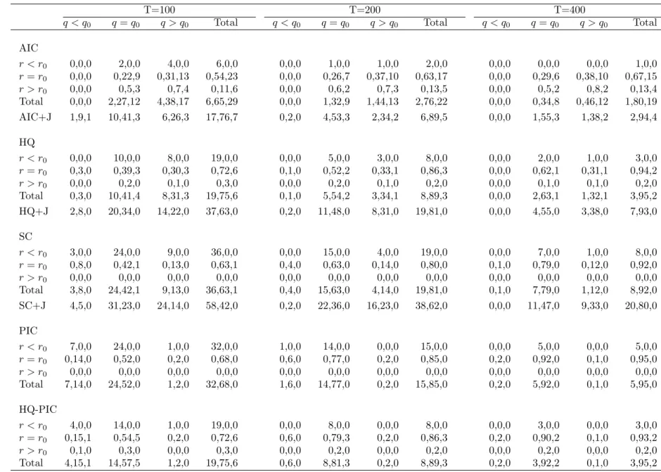
Simulation results are reported in “three-dimensional” frequency tables. The columns correspond to
the percentage of times the selected models had cointegrating rank smaller than the true rank(q < q0),
information about the rank of short-run dynamics r. Information about the lag-length is provided
within each cell, where the entry is disaggregated on the basis of p. The three numbers provided in
each cell, from left to right, correspond to percentages with lag lengths smaller than the true lag, equal
to the true lag and larger than the true lag. The ‘Total’ column on the right margin of each table
provides information about marginal frequencies ofpand r only. The row titled ‘Total’ on the bottom
margin of each table provides information about the marginal frequencies of pand q only. Finally, the
bottom right cell provides marginal information about the lag-length choice only.
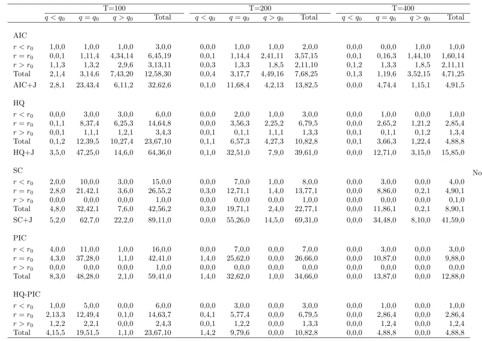
We report results of two sets of 100 DGPs. Table 1 summarises the model selection results for 100
DGPs that have one lag in di¤erences with a short-run rank of one and cointegrating rank of two, i.e.,
(p0; r0; q0) = (1;1;2). Table 2 summarises the model selection results for 100 DGPs that have two lags
in di¤erences with a short-run rank of one and cointegrating rank of one (p0; r0; q0) = (2;1;1). These
two groups of DGPs are contrasting in the sense that the second group of DGPs have more severe
restrictions in comparison to the …rst one.
The …rst three panels of the tables correspond to all model selection based on the traditional model
selection criteria. The additional bottom row for each of these three panels provides information about
the lag-length and the cointegrating rank, when the lag-length is chosen using the simple version of
that model selection criterion and the cointegrating rank is chosen using the Johansen procedure,
and in particular the sequential trace test with 5% critical values that are adjusted for sample size.
Comparing the rows labelled ‘AIC+J’, ‘HQ+J’ and ‘SC+J’, we conclude that the inference about q
is not sensitive to whether the selected lag is correct or not. In Table 1 all three criteria choose the
correctq approximately 54%, 59% and 59% of the time for sample sizes 100, 200 and 400, respectively.
In Table 2 all three criteria choose the correct q approximately 70%, 82% and 82% of the time for
sample sizes 100, 200 and 400, respectively.
From the …rst three panels of Table 1 we can clearly see that traditional model selection criteria do
not perform well in choosing p; r andq jointly in …nite samples. The percentages of times the correct
model is chosen are only 22%, 26% and 29% with the AIC, 39%, 52% and 62% with HQ, and 42%,
63% and 79% with SC, for sample sizes of 100, 200 and 400, respectively. Note that when we compare
the marginal frequencies of (p; r), HQ is the most successful for choosing both p and r, a conclusion
that is consistent with results in Vahid and Issler (2002).
The main reason for not being able to determine the triplet(p; r; q)correctly is the failure of these
criteria to choose the correct q. Ploberger and Phillips (2003) show that the correct penalty for free
parameters in the long-run parameter matrix is larger than the penalty considered by traditional model
selection criteria. Accordingly, all three criteria are likely to over-estimate q in …nite samples, and of
parameters, even though the penalty is still less than ideal. This is exactly what the simulations reveal.
The fourth panel of Table 1 includes results for the PIC. The percentages of times the correct model
is chosen increase to 52%, 77% and 92% for sample sizes of 100, 200 and 400, respectively. Comparing
the margins, it becomes clear that this increased success relative to HQ and SC is almost entirely due
to improved precision in the selection ofq. The PIC choosesq correctly 76%, 91% and 97% of the time
for sample sizes 100, 200 and 400, respectively. Furthermore, for the selection of p and r only, PIC
does not improve upon HQ.
Similar conclusions can be reached from the results for the (2;1;1) DGPs presented in Table 2.
We note that in this case, even though the PIC improves on HQ and SC in choosing the number
of cointegrating vectors, it does not improve on HQ or SC in choosing the exact model, because it
severely underestimates p. This echoes the …ndings of Vahid and Issler (2002) in the stationary case
that the Schwarz criterion (recall that the PIC penalty is of the same order as the Schwarz penalty in
the stationary case) severely underestimates the lag length in small samples in reduced rank VARs.
Our Monte-Carlo results show that the advantage of PIC over HQ and SC is in the determination
of the cointegrating rank. Indeed, HQ seems to have an advantage over PIC in selecting the correct p
and r in small samples. These results coupled with the practical di¢culties in computing the PIC we
outline in Section 4 motivated us to consider the two-step alternative procedure to improve the model
selection task.
The …nal panels in Tables 1 and 2 summarise the performance of our two-step procedure. In both
tables we can see that the hybrid HQ-PIC procedure improves on all other criteria in selecting the
exact model. The improvement is a consequence of the advantage of HQ in selecting p and r better,
and PIC in selecting q better.
Note that our hybrid procedure results in over-parameterised models more often than just using PIC
as the model selection criterion. We examined whether this trade-o¤ has any signi…cant consequences
for forecasting and found that it does not. In all simulation settings, models selected by the hybrid
procedure with HQ-PIC as the model selection criteria forecast better than models selected by PIC.
Again, we do not present these results here, but they are also available upon request.
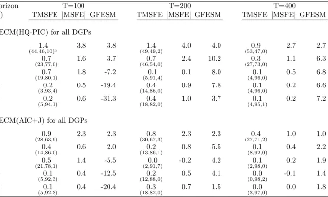
6.2 Forecasts
Recall that the forecasting results are expressed as the percentage improvement in forecast accuracy
measures of possibly rank reduced models over the unrestricted VAR model in levels selected by SC.
Also, note that the object of interest in this forecasting exercise is assumed to be the …rst di¤erence of
variables, although GFESM gives a measure of accuracy that is the same for levels or di¤erences.
by the iterative process of Section 3 as VECM(HQ-PIC). We label the models estimated by the usual
Johansen method with AIC as the model section criterion for the lag order as VECM(AIC+J).
Table 3 presents the forecast accuracy improvements in a (1;1;2) setting. In terms of the trace
and determinant of the MSFE matrix, there is some improvement in forecasts over unrestricted VAR
models at all horizons. With only 100 observations, GFESM worsens for horizons 8 and longer. This
means that if the object of interest was some combination of di¤erences across di¤erent horizons (for
example, the levels of all variables or the levels of some variables and …rst di¤erences of others), there
may not have been any improvement in the MSFE matrix. With 200 or more observations, all forecast
accuracy measures show some improvement, with the more substantial improvements being for the
one-step-ahead forecasts. Also note that the forecasts of the models selected by the hybrid procedure
are almost always better than those produced by the model chosen by the AIC plus Johansen method,
which only pays attention to lag-order and long-run restrictions.
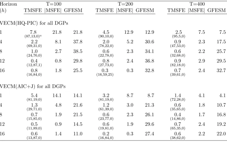
Table 4 presents the forecast accuracy improvements in a(2;1;1) setting. This set of DGPs have
more severe rank reductions than the (1;1;2) DGPs, and, as a result, the models selected by the
hybrid procedure show more substantial improvements in forecasting accuracy over the VAR in levels,
in particular for smaller sample sizes. Forecasts produced by the hybrid procedure are also substantially
better than forecasts produced by the AIC+Johansen method, which does not incorporate short-run
rank restrictions. Note that although the AIC+Johansen forecasts are not as good as the HQ-PIC
forecasts, they are substantially better than the forecasts from unrestricted VARs at short horizons.
Following a request from a referee in Tables 3 and 4 we have also presented Diebold and Mariano
(1995) tests for equal predictive accuracy between the rank reduced speci…cations and the unrestricted
VARs for the TMSFE. In general the results are as expected. Models that incorporate reduced rank
restrictions rarely forecast signi…cantly worse than the unrestricted models. They either perform the
same or signi…cantly better than the unrestricted VARs.
7
Empirical example
The techniques discussed in this paper are applied to two di¤erent data sets in forecasting exercises.
The …rst data set contains Brazilian in‡ation, as measured by three di¤erent types of consumer-price
indices, available on a monthly basis from 1994:9 through 2009:11, with a span of more than 15
years (183 observations). It was extracted from IPEADATA – a public database with downloadable
Brazilian data (http://www.ipeadata.gov.br/). The second data set being analyzed consist of real
U.S. per-capita private output5, personal consumption per-capita, and …xed investment per-capita,
available on a quarterly basis from 1947:1 through 2009:03, with a span of more than 62 years (251
observations). It was extracted from FRED’s database of the Federal Reserve Bank of St. Louis
(http://research.stlouisfed.org/fred2/). Considering that we will keep some observations for forecast
evaluation (90 observations), the size of these data bases are close to the number of simulated
obser-vations in the Monte-Carlo exercise for T = 100and T = 200 respectively.
7.1 Forecasting Brazilian In‡ation
The Brazilian data set consists of three alternative measures of CPI price indices. The …rst is the o¢cial
consumer price index used in the Brazilian In‡ation-Targeting Program. It is computed by IBGE, the
statistics bureau of the Brazilian government, labelled here as CPI-IBGE. The second is the consumer
price index computed by Getulio Vargas Foundation, a traditional private institution which computes
several Brazilian price indices since 1947, labelled here as CPI-FGV. The third is the consumer price
index computed by FIPE, an institute of the Department of Economics of the University of São Paulo,
labelled here as CPI-FIPE.
These three indices capture di¤erent aspects of Brazilian consumer-price in‡ation. First, they di¤er
in terms of geographical coverage. CPI-FGV collects prices in 12 di¤erent metropolitan areas in Brazil,
11 of which are also covered by CPI-IBGE6. On the other hand, CPI-FIPE only collects prices in São
Paulo – the largest city in Brazil – also covered by the other two indices. Tracked consumption bundles
are also di¤erent across indices. CPI-FGV focus on bundles of the representative consumer with income
between 1 and 33 minimum wages. CPI-IBGE focus on bundles of consumers with income between 1
and 40 minimum wages, while CPI-FIPE focus on consumers with income between 1 and 20 minimum
wages.
Although all three indices measure consumer-price in‡ation in Brazil, Granger Causality tests
con…rm the usefulness of conditioning on alternative indices to forecast any given index in the models
estimated here. Despite the existence of these forecasting gains, one should expect a similar pattern
for impulse-response functions across models, re‡ecting a similar response of di¤erent price indices to
shocks to the dynamic system.
We compare the forecasting performance of (i) the VAR in (log) levels, with lag length chosen by
the standard Schwarz criterion; (ii) the VECM, using standard AIC for choosing the lag length and
Johansen’s test for choosing the cointegrating rank; and (iii) the reduced rank model, with rank and lag
length chosen simultaneously using the Hannan-Quinn criterion and cointegrating rank chosen using
PIC, estimated by the iterative process described in Section 3. All forecast comparisons are made using
the …rst di¤erence of the (log) levels of the price indices, i.e., price in‡ation.
For all three models, the estimation sample starts from 1994:09 through 2001:02, with78
observa-tions. With these initial estimates, we compute the applicable choices ofp,r, andq for each model and
forecast in‡ation up to 16 months ahead. Keeping the initial observation …xed (1994:9), we add one
observation at the end of the estimation sample, choose potentially di¤erent values forp,r, andq for
each model, and forecast in‡ation again up to 16 months ahead. This procedure is then repeated until
the …nal estimation sample reaches 1994:9 through 2008:7, with 167 observations. Then, we have a
total of90out-of-sample forecasts for each horizon (1to16months ahead), which are used for forecast
evaluation. Thus, the estimation sample varies from 78 to 167 observations and mimics closely the
simulations labelled T = 100in the Monte-Carlo exercise.
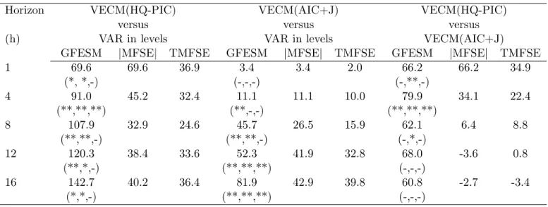
Results of the exercise described above are presented in Table 5. For any horizon, there are
sub-stantial forecasting gains of the VECM(HQ-PIC) over the VAR in levels: for example, for 4 months
ahead, GF ESM, T M SF E and jM SF Ej show gains of 91:0%, 45:2% and 32:4% respectively.
Re-sults for 8 months ahead are even more impressive. Upon comparison, the forecasting gains of the
VECM(AIC+J) over the latter are not as large for the shorter horizons, but it increases substantially
for horizons 12 and 16 as expected. The comparison between VECM(HQ-PIC) and VECM(AIC+J)
shows gains for the former almost everywhere, with substantial improvement in shorter horizons. For4
months ahead, GF ESM,T M SF E andjM SF Ejshow gains of 79:9%,39:0%and 22:4%respectively. Table 5 also shows Diebold-Mariano statistics for equal forecast variances among pair of forecasts
for individual series and all horizons. As a rule, forecasting using the VAR in levels produces signi…cant
higher variances than either the VECM(HQ-PIC) or the VECM(AIC+J). Testing the equality of the
variances of the forecast errors using the VECM(HQ-PIC) and the VECM(AIC+J) show signi…cant
di¤erences at moderate horizons (4 and 8), although, most of the time, we cannot reject the null of
equal variances. It should be noticed that there is no case where either the VAR in levels or the
VECM(AIC+J) generate a smaller signi…cant variance vis-a-vis the VECM(HQ-PIC) for any in‡ation
series at all horizons.
It is also worth reporting the …nal choices of p, r, and q for the best models studied here as the
estimation sample goes from 1994:09-2001:02 all the way to 1994:9-2008:7. While the
VECM(HQ-PIC) chose p = 17, r = 1 or 2, and q = 08, most of the time, the VECM(AIC+J) chose p = 19
and q = 110, most of the time. Hence, the superior performance of the VECM(HQ-PIC) vis-a-vis
the VECM(AIC+J) may be due to either imposing a reduced-rank structure or to ignoring potential
cointegration relationships. This is especially true for the shorter horizons.
7On ocasion it chosep= 3.
8On ocasion it choseq= 1.
9On ocasion it chosep= 5.
7.2 Forecasting U.S. Macroeconomic Aggregates
The data being analyzed here is well known. It consists of (log) real U.S. per-capita private output –
y, personal consumption per-capita – c, and …xed investment per-capita – i, extracted from FRED’s
database on a quarterly frequency11 from 1947:01 through 2009:03.
Again, we compare the forecasting performance of (i) the VAR in (log) levels, with lag length
chosen by the standard Schwarz criterion; (ii) the VECM, using standard AIC for choosing the lag
length and Johansen’s test for choosing the cointegrating rank; and (iii) the reduced rank model, with
rank and lag length chosen simultaneously using the Hannan-Quinn criterion and cointegrating rank
chosen using PIC, estimated by the iterative process of Section 3. All forecast comparisons are made
using the …rst di¤erence of the (log) levels of the data, i.e., using log (yt), log (ct), and log (it).
For all three models, the estimation sample starts from 1947:01 through 1983:02, with146observations.
As before, we keep rolling the estimation sample until it reaches 1947:01 through 2005:03, with 235
observations, with a total of 90 out-of-sample forecasts for each horizon used for forecast evaluation.
Since the estimation sample varies from 146 to 235 observations it mimics closely the simulations
labelled T = 200in the Monte-Carlo exercise.
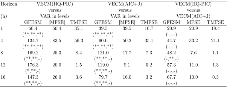
Results of the exercise described above are presented in Table 6. For any horizon, there are
considerable forecasting gains for the VECM(HQ-PIC) over the VAR in levels: at 8 quarters ahead,
GF ESM,T M SF E andjM SF Ejshow gains of169:2%,25:3%and8:4%respectively. The forecasting gains of the VECM(AIC+J) over the VAR in levels are not as large for all horizons. The comparison
between VECM(HQ-PIC) and VECM(AIC+J) shows gains for the former everywhere, with higher
improvement in shorter horizons. For example, at4quarters ahead,GF ESM,T M SF E andjM SF Ej
show gains of 44:8%, 33:3% and 21:4% respectively. Despite that, the Diebold-Mariano statistics for
equal variances for the forecast errors predicting log (yt), log (ct), and log (it) are insigni…cant
everywhere, when VECM(HQ-PIC) and VECM(AIC+J) are confronted.
Finally, we investigate the …nal choices of p, r, and q as the estimation sample progresses from
1947:01-1983:02 to 1947:01-2005:03. For the VECM(HQ-PIC) they are: p = 1, r = 2, and q = 0,
everywhere, while the VECM(AIC+J) chose p= 1 and q= 112, most of the time. Hence, the superior
performance of the VECM(HQ-PIC) vis-a-vis the VECM(AIC+J) may be due to either imposing a
reduced-rank structure or to ignoring potential cointegration relationships.
1 1Using FRED’s mnemonics (2010) for the series, the precise de…nitions are: PCECC96 consumption, FPIC96
-investment, and (GNP96 - FGCEC96) - output. Population series mnemonics is POP, which is only available from 1952 on in FRED. To get a complete series starting in 1947:01 it was chained with the same series available in DRI database, whose mnemonics is GPOP.
8
Conclusion
Motivated by the results of Vahid and Issler (2002) on the success of the Hannan-Quinn criterion in
selecting the lag length and rank in stationary VARs, and the results of Ploberger and Phillips (2003)
and Chao and Phillips (1999) on the generalisation of Rissanen’s theorem to trending time series
and the success of PIC in selecting the cointegrating rank in VARs, we propose a combined HQ-PIC
procedure for the simultaneous choice of the lag-length and the ranks of the short-run and long-run
parameter matrices in a VECM and we prove its consistency. Our simulations show that this procedure
is capable of selecting the correct model more often than other alternatives such as pure PIC or SC.
In this paper we also present forecasting results that show that models selected using this hybrid
procedure produce better forecasts than unrestricted VARs selected by SC and cointegrated VAR
models whose lag length is chosen by the AIC and whose cointegrating rank is determined by the
Johansen procedure. We have chosen these two alternatives for forecast comparisons because we
believe that these are the model selection strategies that are most often used in the empirical literature.
However, we have considered several other alternative model selection strategies and the results are
qualitatively the same: the hybrid HQ-PIC procedure leads to models that generally forecast better
than VAR models selected using other procedures.
A conclusion we would like to highlight is the importance of short-run restrictions for forecasting.
We believe that there has been much emphasis in the literature on the e¤ect of long-run
cointegrat-ing restrictions on forecastcointegrat-ing. Given that long-run restrictions involve the rank of only one of the
parameter matrices of a VECM, and that inference on this matrix is di¢cult because it involves
in-ference about stochastic trends in variables, it is puzzling that the forecasting literature has paid so
much attention to cointegrating restrictions and relatively little attention to lag-order and short-run
restrictions in a VECM. The present paper …lls this gap and highlights the fact that the lag-order
and the rank of short-run parameter matrices are also important for forecasting. Our hybrid model
selection procedure and the accompanying simple iterative procedure for the estimation of a VECM
with long-run and short-run restrictions provide a reliable methodology for developing multivariate
autoregressive models that are useful for forecasting.
How often restrictions of the type considered in this paper are present in VAR approximations to
real life data generating processes is an empirical question. Macroeconomic models in which trends
and cycles in all variables are generated by a small number of dynamic factors …t in this category.
Also, empirical papers that study either regions of the same country or similar countries in the same
region often …nd these kinds of long-run and short-run restrictions. We illustrate the usefulness of the
and U.S. macroeconomic aggregates growth rates. We …nd gains of imposing short- and long-run
restrictions in VAR models, since the VECM(HQ-PIC) and the VECM(AIC+J) outperform the VAR in
levels everywhere. Tests of equal variance con…rm that these gains are signi…cant. Moreover, ignoring
short-run restrictions usually produce inferior forecasts with these data, since the VECM(HQ-PIC)
outperforms the VECM(AIC+J) almost everywhere, but these gains are not always signi…cant in tests
of equal variance.
It is true that discovering the “true” model is a di¤erent objective from model selection for
fore-casting. However, in the context of partially non-stationary variables, there are no theoretical results
that lead us to a de…nite model selection strategy for forecasting. Using a two variable example,
El-liott (2006) shows that, ignoring estimation uncertainty, whether or not considering cointegration will
improve short-run or long-run forecasting depends on all parameters of the DGP, even the parameters
of the covariance matrix of the errors. In addition there is no theory that tells us whether …nite sample
biases of parameter estimates will help or hinder forecasting in partially non-stationary VARs. Given
this state of knowledge, when one is given the task of selecting a single model for forecasting it is
reasonable to use a model selection criterion that is more likely to pick the “true” model and in this
paper we verify that VARs selected by our hybrid model selection strategy are likely to produce better
forecasts than unrestricted VARs and VARs that only incorporate cointegration restrictions.
References
Ahn, S. K. & Reinsel, G. C. (1988), ‘Nested reduced-rank autoregressive models for multiple time
series’,Journal of the American Statistical Association 83, 849–856.
Anderson, H. & Vahid, F. (1998), ‘Testing multiple equation systems for common nonlinear
compo-nents’,Journal of Econometrics84, 1–36.
Anderson, T. (1951), ‘Estimating linear restrictions on regression coe¢cients for multivariate normal
distributions’,Annals of Mathematical Statistics 22, 327–351.
Athanasopoulos, G. & Vahid, F. (2008), ‘VARMA versus VAR for macroeconomic forecasting’,Journal
of Business and Economic Statistics26, 237–252.
Aznar, A. & Salvador, M. (2002), ‘Selecting the rank of the cointegation space and the form of the
intercept using an information criterion’,Econometric Theory 18, 926–947.
Centoni, M., Cubbada, G. & Hecq, A. (2007), ‘Common shocks, common dynamics and the
Chao, J. & Phillips, P. (1999), ‘Model selection in partially nonstationary vector autoregressive
processes with reduced rank structure’,Journal of Econometrics91, 227–271.
Christo¤ersen, P. & Diebold, F. (1998), ‘Cointegration and long-horizon forecasting’,Journal of
Busi-ness and Economic Statistics16, 450–458.
Clements, M. P. & Hendry, D. F. (1993), ‘On the limitations of comparing mean squared forecast errors
(with discussion)’,Journal of Forecasting 12, 617–637.
Clements, M. P. & Hendry, D. F. (1995), ‘Forecasting in cointegrated systems’, Journal of Applied
Econometrics10, 127–146.
Diebold, F. X. & Mariano, R. S. (1995), ‘Comparing predictive accuracy’, Journal of Business and
Economic Statistics13, 253–263.
Elliott, G. (2006), Forecasting with trending data, in G. Elliott, C. Granger & A. Timmermann, eds,
‘Handbook of Economic Forecasting’, Vol. 1, Elsevier, chapter 11, pp. 555–604.
URL:http://ideas.repec.org/h/eee/ecofch/1-11.html
Engle, R. F. & Yoo, S. (1987), ‘Forecasting and testing in cointegrated systems’, Journal of
Econo-metrics35, 143–159.
Gonzalo, J. & Pitarakis, J. (1995), ‘Speci…cation via model selection in vector error correction models’,
Economic Letters60, 321–328.
Gonzalo, J. & Pitarakis, J.-Y. (1999), Dimensionality e¤ect in cointegration tests, in R. Engle &
H. White, eds, ‘Cointegration, Causality and Forecasting: A Festschrift in Honour of Clive W. J.
Granger’, New York: Oxford University Press, chapter 9, pp. 212–229.
Gourieroux, C. & Peaucelle, I. (1992), ‘Series codependantes application a l’hypothese de parite du
pouvoir d’achat’,Revue d’Analyse Economique68, 283–304.
Hecq, A., Palm, F. & Urbain, J.-P. (2006), ‘Common cyclical features analysis in VAR models with
cointegration’,Journal of Econometrics132, 117–141.
Ho¤man, D. & Rasche, R. (1996), ‘Assessing forecast performance in a cointegrated system’, Journal
of Applied Econometrics11, 495–517.
Johansen, S. (1988), ‘Statistical analysis of cointegrating vectors’,Journal of Economic Dynamics and
Johansen, S. (1991), ‘Estimation and hypothesis testing of cointegration vectors in gaussian vector
autoregressive models’,Econometrica 59, 1551–1580.
Leeb, H. & Potscher, B. (2005), ‘Model selection and inference: Facts and …ction’,Econometric Theory
21, 21–59.
Lin, J. L. & Tsay, R. S. (1996), ‘Cointegration constraints and forecasting: An empirical examination’,
Journal of Applied Econometrics11, 519–538.
Lütkepohl, H. (1985), ‘Comparison of criteria for estimating the order of a vector autoregressive
process’,Journal of Time Series Analysis 9, 35–52.
Lütkepohl, H. (1993),Introduction to Multiple Time Series Analysis, 2nd edn, Springer-Verlag,
Berlin-Heidelberg.
Magnus, J. R. & Neudecker, H. (1988),Matrix Di¤erential Calculus with Applications in Statistics and
Econometrics, New York: John Wiley and Sons.
Paulsen, J. (1984), ‘Order determination of multivariate autoregressive time series with unit roots’,
Journal of Time Series Analysis5, 115–127.
Phillips, P. C. B. (1996), ‘Econometric model determination’,Econometrica 64, 763–812.
Phillips, P. C. B. & Hansen, B. (1990), ‘Statistical inference in instrumental variables regression with
I(1) processes’,Review of Economic Studies57, 99–125.
Phillips, P. C. B. & Loretan, M. (1991), ‘Estimating long-run economic equilibria’,Review of Economic
Studies58, 407–436.
Phillips, P. & Ploberger, W. (1996), ‘An asymptotic theory of Bayesian inference for time series’,
Econometrica64, 381–413.
Ploberger, W. & Phillips, P. C. B. (2003), ‘Empirical limits for time series econometric models’,
Econo-metrica71, 627–673.
Poskitt, D. S. (1987), ‘Precision, complexity and bayesian model determination’,Journal of the Royal
Statistical Society B49, 199–208.
Quinn, B. (1980), ‘Order determination for a multivariate autoregression’, Journal of the Royal
Sta-tistical Society B42, 182–185.
Rissanen, J. (1987), ‘Stochastic complexity’,Journal of the Royal Statistical Society B49, 223–239.
Saikkonen, P. (1992), ‘Estimation and testing of cointegrated systems by an autoregressive
approxima-tion’,Econometric Theory 8, 1–27.
Silverstovs, B., Engsted, T. & Haldrup, N. (2004), ‘Long-run forecasting in multicointegrated systems’,
Journal of Forecasting23, 315–335.
Sims, C., Stock, J. & Watson, M. (1990), ‘Inference in linear time series models with some unit roots’,
Econometrica58, 113–144.
Tsay, R. (1984), ‘Order selection in nonstationary autoregressive models’,Annals of Statistics12, 1425–
1433.
Vahid, F. & Engle, R. F. (1993), ‘Common trends and common cycles’,Journal of Applied Econometrics
8, 341–360.
Vahid, F. & Issler, J. V. (2002), ‘The importance of common cyclical features in VAR analysis: A
Monte-Carlo study’,Journal of Econometrics109, 341–363.
Velu, R., Reinsel, G. & Wickern, D. (1986), ‘Reduced rank models for multiple time series’,Biometrika
73, 105–118.
Wallace, C. (2005),Statistical and Inductive Inference by Minimum Message Length, Berlin: Springer.
Wallace, C. & Freeman, P. (1987), ‘Estimation and inference by compact coding’,Journal of the Royal
Statistical Society B49, 240–265.
A
The Fisher information matrix of the reduced rank VECM
Assuming that the …rst observation in the sample is labelled observation p+ 1 and that the sample
containsT +p observations, we write theK-variable reduced rank VECM
yt= 0 Iq 0 yt 1+ CIr0 [D1 yt 1+D2 yt 2+ +Dp yt p] + +et;
or in stacked form
Y =Y 1 Iq +W D Ir C + T 0
where
Y T K =
2 6 4 y0 1 .. . y0 T 3 7
5; Y 1 T K = 2 6 4 y0 0 .. . y0 T 1 3 7
5; TEK = 2 6 4 e0 1 .. . e0 T 3 7 5 W
T Kp = Y 1 Y p =
2 6 4 y0 0 y 0 p+1 .. . ... ... y0
T 1 y
0 T p 3 7 5 D Kp r =
0 B @ D0 1 .. . D0 p 1 C A;
and T is a T 1 vector of ones. When et are N(0; ) and serially uncorrelated, the log-likelihood
function, conditional on the …rst p observations being known, is:
lnl( ; !) = KT
2 ln (2 ) T
2 lnj j 1 2
T X
t=1
e0t 1et
= KT
2 ln (2 ) T
2 lnj j 1 2tr E
1E0 ; where = 0 B B B B @
vec( ) vec( ) vec(D) vec(C)
1 C C C C A
is a(K q)q+Kq+Kpr+r(K r)+Kmatrix of mean parameters, and!=vech( )is aK(K+ 1)=2
vector of unique elements of the variance matrix. The di¤erential of the log-likelihood is (see Magnus
and Neudecker 1988)
dlnl( ; !) = T 2tr
1d +1 2tr
1d 1E0
E 1
2tr
1E0
dE 1 2tr
1dE0 E
= 1
2tr
1 E0
E T 1d tr 1E0dE ;
and the second di¤erential is:
d2lnl( ; !) = tr d 1 E0E T 1d +1 2tr
1 2E0
dE T d 1d
tr d 1E0dE tr 1dE0dE :
Since we eventually want to evaluate the Fisher information matrix at the maximum likelihood
esti-mator, and at the maximum likelihood estimatorE^0^
E T^ = 0;and also ^ 1E^0
apparent from the …rst di¤erentials), we can delete these terms from the second di¤erential, and use
tr(AB) =vec(A0
)0vec(B) to obtain
d2lnl( ; !) = T 2tr
1d 1d tr 1dE0
dE
= T
2 (d!) 0
D0K 1 1 DKd! (vec(dE))
0 1
IT vec(dE);
whereDK is the “duplication matrix”. From the model, we can see that
dE= Y 1 d0 Y 1 Iq d W dD Ir C W D 0 dC Td 0
;
and therefore
vec(dE) = 0
Y(2)1 IK Y 1 Iq CIr0 W
0
IK r W D IK T d :
Hence, the elements of the Fisher information matrix are:
F IM11 = 1 0
Y(2)10Y(2)1; F IM12= 1 Y(2) 0
1 Y 1 Iq ;
F IM13 = 1 Ir
C0 Y (2)0
1 W; F IM14= 1 0
IK r Y (2)0
1 W D
F IM15 = 1 Y(2) 0 1 T
F IM22 = 1 Iq 0 Y01Y 1 Iq ; F IM23= 1 Ir
C0 Iq 0
Y01W
F IM24 = 1 I 0 K r
Iq 0
Y01W D; F IM25= 1 Iq 0 Y 0
1 T
F IM33 = Ir C 1 CIr0 W 0
W; F IM34= Ir C 1 IK r0 W 0
W D
F IM35 = Ir C 1 W 0
T
F IM44 = 0 IK r 1 IK r0 D 0
W0W D; F IM45= 0 IK r 1 D 0
W0 T F IM55 = 1 0T T = 1 T
B
Proof of Theorem 2
The …rst three assumptions ensure that ytis covariance stationary andytare cointegrated with
coin-tegrating rankq0:These together with assumption (vi) ensure that all sample means and covariances of
ytconsistently estimate their population counterparts and the least squares estimator of parameters
is consistent. Assumptions (iv) and (v) state that the true rank is r0 and the true lag-length isp0 (or
the lag order of the implied VAR in levels isp0+ 1). For any(p; r)pair, the second step of the analysis
Anderson (1951). Reinsel (1997) contains many of the results that we use in this proof). Under the
assumption of normality, these are the ML estimates of 1; : : : ; p with rankr with unrestricted and
the resulting ^p;r used in the HQ procedure is the corresponding ML estimate of . Note that
normal-ity of the true errors is not needed for the proof. We use the results of Sims et al. (1990) who show that
in the above model the least squares estimates of 1; : : : ; p have the standard asymptotic properties
as in stationary VARs, in particular that they consistently estimate their population counterparts and
that their rate of convergence is the same as T 12: Let z
t; zt 1; : : : ; zt p denote yt; yt 1; :::; yt p
after the in‡uence of the constant and yt 1 is removed from them and let Z; Z 1; : : : ; Z p denote
T Kmatrices withz0
t; z 0
t 1; : : : ; z 0
t p in their rowt= 1; : : : ; T (we assume that the sample starts from
t= pmax+ 1), and letWp= [Z 1... ...Z p]andBp= [ 1... ... p]0. The estimated model in the second
step can be written as:
Z =WpB^p+ ^Up
where Up^ is the T K matrix of residuals when the lag length is p. In an unrestricted regression
lnjT1U^0
pUp^ j= lnjT1(Z 0
Z Z0
Wp(W0
pWp) 1W 0
pZ)j= lnjT1Z 0
Zj+ lnjIK (Z0
Z) 1Z0
Wp(W0
pWp) 1W 0 pZj = lnjT1Z0
Zj+PKi=1ln(1 ^2i(p));where ^12(p) ^22(p) : : : ^2K(p);the eigenvalues of (Z0
Z) 1Z0
Wp(W0
pWp) 1W 0
pZ are the ordered sample partial canonical correlations between yt and
yt 1; :::; yt p after the in‡uence of a constant and yt 1 has been removed. Under the restriction
that the rank of B is r; the log-determinant of the squared residuals matrix becomes lnjT1U^0
p;rU^p;rj= lnjT1Z0
Zj+PKi=K r+1ln(1 ^2i(p)): Further, note thatWp = [Wp 1...Z p] and from the geometry of
least squares we know
Z0 Wp(W0
pWp) 1W 0 pZ =Z
0
Wp 1(Wp0 1Wp 1) 1Wp0 1Z+Z 0
Qp 1Z p(Z0 pQp 1Z p) 1Z0 pQp 1Z where Qp 1 =IT Wp 1(Wp0 1Wp 1) 1Wp0 1:
(i) Consider p=p0 and r=r0 1 : lnjT1U^p00;r0 1
^
Up0;r0 1j lnj
1 TU^
0 p0;r0
^
Up0;r0j= ln(1 ^
2
K r0+1(p0)):
^2
K r0+1(p0) converges in probability to its population counterpart, the r0-th largest eigenvalue of
1 z B
0
p0 wBp0; where x denotes the population second moment of the vector x. This population
canonical correlation is strictly greater than zero becauseBp0 has rank r0:Therefore
plim (lnjT1U^0
p0;r0 1Up^ 0;r0 1j lnj
1 TU^
0
p0;r0Up^ 0;r0j) = ln(1
2
K r0+1(p0))>0:
(ii) Consider p=p0 1 and r=r0:
(Z0
Z) 1Z0
Wp0(W
0 p0Wp0)
1W0
p0Z = (Z
0
Z) 1Z0
Wp0 1(W
0
p0 1Wp0 1)
1W0 p0 1Z
+(Z0Z) 1Z0Qp0 1Z p0(Z
0
p0Qp0 1Z p0)
1Z0