www.the-cryosphere.net/6/729/2012/ doi:10.5194/tc-6-729-2012
© Author(s) 2012. CC Attribution 3.0 License.
The Cryosphere
Laboratory study of initial sea-ice growth: properties of grease ice
and nilas
A. K. Naumann1, D. Notz1, L. H˚avik2, and A. Sirevaag2
1Max Planck Institute for Meteorology, Hamburg, Germany 2Geophysical Institute, University of Bergen, Bergen, Norway Correspondence to:A. K. Naumann ([email protected])
Received: 23 December 2011 – Published in The Cryosphere Discuss.: 13 January 2012 Revised: 26 May 2012 – Accepted: 12 June 2012 – Published: 10 July 2012
Abstract.We investigate initial sea-ice growth in an ice-tank study by freezing an NaCl solution of about 29 g kg−1 in
three different setups: grease ice grew in experiments with waves and in experiments with a current and wind, while ni-las formed in a quiescent experimental setup. In this paper we focus on the differences in bulk salinity, solid fraction and thickness between these two ice types.
The bulk salinity of the grease-ice layer in our experiments remained almost constant until the ice began to consolidate. In contrast, the initial bulk-salinity evolution of the nilas is well described by a linear decrease of about 2.1 g kg−1h−1
independent of air temperature. This rapid decrease can be qualitatively understood by considering a Rayleigh number that became maximum while the nilas was still less than 1 cm thick.
Comparing three different methods to measure solid frac-tion in grease ice based on (a) salt conservafrac-tion, (b) mass conservation and (c) energy conservation, we find that the method based on salt conservation does not give reliable re-sults if the salinity of the interstitial water is approximated as being equal to the salinity of the underlying water. Instead the increase in salinity of the interstitial water during grease-ice formation must be taken into account. In our experiments, the solid fraction of grease ice was relatively constant with values of 0.25, whereas it increased to values as high as 0.50 as soon as the grease ice consolidated at its surface. In con-trast, the solid fraction of the nilas increased continuously in the first hours of ice formation and reached an average value of 0.55 after 4.5 h.
The spatially averaged ice thickness was twice as large in the first 24 h of ice formation in the setup with a current and wind compared to the other two setups, since the wind kept
parts of the water surface ice free and therefore allowed for a higher heat loss from the water. The development of the ice thickness can be reproduced well with simple, one dimen-sional models that only require air temperature or ice surface temperature as input.
1 Introduction
Sea-ice growth in turbulent water differs from sea-ice growth in quiescent water. In turbulent water, ice crystals accumulate at the surface, forming a grease-ice layer composed of indi-vidual ice crystals and small irregular clumps of ice crystals. In quiescent conditions, nilas, a thin elastic crust, forms at the surface, which thickens as water molecules freeze to the ice–water interface (see e.g. Martin, 1981; Weeks and Ack-ley, 1986). To gain a better understanding of the differences in initial sea-ice formation in turbulent and quiescent water, we conducted an ice-tank study focusing on the evolution of new sea ice.
at a critical solid fraction. Studies with a multidisciplinary focus have been described by Haas et al. (1999) and Wilkin-son et al. (2009). Analysing the first study, Smedsrud (2001) found considerable temporal variability in frazil-ice concen-tration for a low absolute frazil concenconcen-tration of around 1 %. Analysis of the latter study by De la Rosa et al. (2011) and De la Rosa and Maus (2012) gave results similar to those of Martin and Kauffman (1981), namely that a critical solid fraction exists at which grease ice transforms to pancake ice. Dai et al. (2004) and Shen et al. (2004) focused on pancake ice and found that pancake ice thickness is influenced by raft-ing processes and that the pancake diameter is determined by the amplitude of the waves.
One of the few field campaigns related to grease-ice prop-erties was carried out by Smedsrud and Skogseth (2006). They found that grease-ice properties vary considerably more than had been anticipated before, measuring solid-fraction values between 0.16 and 0.32. Based primarily on these ob-servations, Smedsrud (2011) suggested a parameterization of grease-ice thickness as a function of wind and current speed. The measurements of the solid fraction of the grease ice by Smedsrud and Skogseth (2006) were based on the salinity method that we describe in Sect. 2.2. Maus and De la Rosa (2012) reviewed this sampling procedure in some detail, and found that a comparison of results obtained from salinity measurements of sieved grease-ice samples remains prob-lematic due to the unknown relationship between the sieved and the bulk salinity of a sample.
To answer some of the questions that remained open from these previous studies, we here describe experiments of ice formation in a tank in which both a quiescent and two differ-ent turbuldiffer-ent setups were realised. Through such a compar-ative experimental study, we are able to directly investigate differences and similarities of sea-ice formation in quiescent and turbulent water. In the experiments, we changed the air temperature systematically to examine its influence on the properties of the forming sea ice. Analysing the properties of sea ice, we focus on its bulk salinity, solid fraction and thick-ness. To determine the solid fraction of the grease-ice layer, we used and compare three different methods.
This paper is structured as follows: in Sect. 2 we describe the experimental setup and the three methods used to deter-mine the solid fraction of the grease-ice layer. Thereafter, in Sect. 3, we give an overview of both the visible evolution of the ice layer and the measured development of the tempera-ture and the salinity of the water underneath the ice during the experiments. In Sect. 4 we first analyse the three meth-ods used to measure solid fraction in grease ice. Then we describe and discuss the bulk salinity and the solid fraction of grease ice and of nilas separately, and in the end compare the properties of these two ice types. Finally, in Sect. 5 we give some concluding remarks.
2 Experimental setup
2.1 Tank setup
The experiments were conducted in a glass tank within a cold room. The tank had a height of 120 cm, a floor area of 194 cm×66 cm and was filled up to 90 cm height with NaCl solution. In total 17 experiments were conducted at fixed air temperatures between −5◦C and−20◦C and each experi-ment lasted for 5 h to 48 h. The initial salinity of the water was about 29 g kg−1, but due to sample collection and
evap-oration it varied between 28.7 g kg−1and 30.6 g kg−1.
To restrict heat loss primarily to the surface area of the tank, 5 cm thick styrodur plates were fixed to the bottom and side walls of the tank. Heating plates that extended about 5 cm above and 18 cm below the water surface were mounted to the sides of the tank at the height of the water surface to prevent the ice from freezing to the walls. Additionally, a heating wire was installed at the bottom of the tank to pre-vent ice formation at the instruments due to supercooling.
We carried out a number of experiments with three differ-ent setups: six quiescdiffer-ent experimdiffer-ents, four experimdiffer-ents with waves and seven experiments with current and wind. In the quiescent experiments, no movement was induced to the wa-ter in the tank (see Fig. 1b). For the experiments with waves, two pumps were adjusted to the resonance frequency of the tank, generating a standing wave with an amplitude of about 5 cm. In the experiments with current and wind, a plate di-vided the tank into two basins at the bottom but allowed for a clockwise water circulation in the uppermost 30 cm (see Fig. 1a). The water was kept moving by both a pump and a wind generator. To avoid freezing of the pump, it was not placed at the surface but beneath the expected ice layer, thus inducing a maximum water velocity at 16 cm depth. A wind generator was installed 10 cm above the water surface to in-duce a surface current. The wind was proin-duced by pressur-ized air that was released through a series of small holes in two horizontally mounted pipes at the beginning of the tank’s linear long sections (see Fig. 1a).
The tank was equipped with 4 CTDs (Conductivity, Tem-perature and Depth; SBE 37-SM MicroCAT) that measured salinity and temperature of the water at different depths (see Table 1). Because the CTDs were calibrated to measure sea-water salinity, but were used to measure NaCl-solution salin-ity, conversion calculations had to be made. By preparing NaCl solutions of known salinity, we found that the differ-ence 1S of sea-water salinity measured by the CTDSCTD
and the true NaCl-solution salinity SNaCl is a function of the temperature Tw and the salinity of the water, giving
1S=SCTD−SNaCl=0.0517SCTD−0.0079Tw. In the tem-perature and salinity range used here this conversion corre-sponds to a subtraction of values between1S=1.2 g kg−1
and1S=1.8 g kg−1from the sea-water salinity values
Fig. 1. (a)Sketch of the experimental setup of the tank during the experiments with current and wind. The instruments shown and the tank setup are discussed in Sect. 2. The instrumental setup in the quiescent experiments and the experiments with waves was similar. Additionally, a turbulent instrument cluster was installed during the experiments (not shown).(b)Picture of the tank during a quiescent experiment.
(c)Pancake ice in an experiment with waves.(d)Grease ice accumulating in one end of the tank in an experiment with current and wind.
Table 1.CTD sensor depths during the different general setups.
CTD quiescent with waves with current and wind
top 8 cm 8 cm 8 cm
middle 32 cm 38 cm 44 cm
bottom 62 cm 74 cm 71 cm
floor 85 cm 85 cm 85 cm
Thermistors (2.2K3A1 Series 1 Thermistors, accuracy of 0.05 K) gave a vertical temperature profile with a resolution of up to 0.5 cm in the ice layer, the air layer above the ice and the water layer below the ice. An additional thermome-ter (Young Platinum Temperature Probe, Model 41342)
recorded the air temperature at 12 cm height above the ice surface. In the quiescent experiments, the ice thickness was read visually from a ruler that was fixed to the side wall of the tank. The setup of the instruments in the tank is shown in Fig. 1a for the experiments with current and wind. For the quiescent experiments and the experiments with waves the instrumental setup was similar, but the dividing wall was re-moved.
2.2 Methods of solid-fraction measurement
In the experiments with waves and with current and wind, samples of the grease-ice layer were taken to measure the solid mass fraction of the ice layer. This solid fraction,φ, is defined as the ratio of the mass of pure ice in the ice layer,
mi, to the total mass of the ice layer,mt: φ=mi
mt. (1)
We used three methods to determine the solid fraction of the ice layer. The first relies on conservation of salt, the second on conservation of mass and the third on conservation of en-ergy.
The most commonly used method to measure the solid fraction in a grease-ice layer is based on conservation of salt (e.g., Smedsrud, 2001), in the following referred to as the salinity method. During melting of the sample, its salt and mass are conserved. Mass conservation givesmt=mi+mw, wheremwis the mass of the interstitial water in the ice layer. Salt conservation givesmtSt=miSi+mwSw, whereStis the salinity of the melted sample,Swis the salinity of the
inter-stitial water andSi=0 g kg−1is the salinity of the pure ice.
For the solid fraction this leads to
φ=Sw−St
Sw . (2)
St was measured directly in the melted sample (with
a Hach HQ40d conductivity sensor), but an assumption has to be made for the salinity of the interstitial water, Sw.
A commonly used assumption is that the salinity of the in-terstitial water between the ice crystals is equal to the salin-ity of the water under the ice layer (e.g., Smedsrud, 2001), which was here measured with the uppermost CTD. This as-sumption is, however, generally not justified because salt is rejected to the interstitial water when ice crystals are form-ing. The salinity of the interstitial water therefore increases during ice formation. In the following, we introduce a sec-ond and a third method, which are independent of salinity, to estimate the accuracy of the salinity method.
The second method to determine the solid fraction is based on the volume difference of the sample before and after melt-ing. We hence refer to it as the volume method. Mass conser-vation givesV2ρw,2=V1ρiφ+V1ρw,1(1−φ), whereV1and V2are the volume andρw,1 andρw,2are the density of the
sample before and after melting, respectively. The density of the sample water is calculated depending on the salinity and the temperature of the sample according to Fofonoff and Mil-lard Jr (1983).ρi=917 kg m−3is the density of pure ice. For
the solid fraction this leads to
φ= V2
V1ρw,2−ρw,1 ρi−ρw,1
. (3)
The third method to determine the solid fraction of the ice layer is based on energy conservation, using a calorime-ter. We therefore call this method calorimeter method. The
calorimeter consisted of a well isolated small bucket with a heating wire and a stirrer inside, and a lid on top. The heat loss to the side walls was negligible (as confirmed by inde-pendent measurements), and the ice-water sample was con-tinuously stirred to ensure an even distribution of the heat added to the sample. The heating wire of the calorimeter supplied an amount of heat1Q to the sample that equals the product of the potentialU, the amperageI and the time during which the wire was active1t. The supplied amount of heat melted the ice and warmed the sample by the tem-perature difference 1T. Energy conservation gives 1Q=
U I 1t=mtcp1T +Lmtφ, where cp=4010 J kg−1K−1 is the specific heat capacity of salt water atT =0◦C andS=
29.9 g kg−1(Bromley et al., 1967) andL=332 300 J kg−1is
the heat of fusion for ice atT = −1.8◦C (Notz, 2005). For
the solid fraction this leads to
φ=U I 1t
−mtcp1T
Lmt
. (4)
The error due to measurement uncertainties according to Gauß’s error propagation law is1φ=0.03 for the salinity method and1φ=0.02 for the calorimeter method (see Ta-ble 2). Note that this small value for the error of the salinity method does not include the uncertainty in the salinity of the interstitial water. For the volume method the error is as large as 1φ=0.24 due to the small difference in volume of the sample before and after melting compared to the total vol-ume of the sample.
2.3 Sampling method
To measure the solid fraction we took samples of the grease-ice layer every half hour during the first hours of the experi-ments with waves and with current and wind. Since the dif-ferent methods required difdif-ferent processing of the samples, not all three methods could be carried out on a single sample. We therefore took two samples at each time. The first one was analysed with the calorimeter and the salinity method and the second one with the volume and the salinity method.
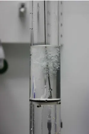
In the experiments with waves, the samples were taken in the middle of the tank. In the experiments with current and wind, the ice crystals first accumulated at the ends of the tank, which is why we shifted the region of sampling to one end of the tank. The sampling device we used was a pipe with a circular plate in the lower part that could be moved from a vertical position to a horizontal position with an attached stick (see Fig. 2). After lowering the pipe into the grease-ice layer, the pipe was sealed by moving the circular plate into a horizontal position with the stick. The pipe could then be lifted out of the tank and the sample was decanted into a graduated measuring glass or the bucket of the calorimeter to be processed further following the methods described in Sect. 2.2.
Fig. 2.Photo of the sampling device with the circular plate in hori-zontal position keeping the sampled grease ice trapped in the pipe.
contained some of the underlying water (Fig. 2). In order to obtain the solid fraction of the grease-ice layer (in con-trast to the solid fraction of the whole sample), the solid fraction of the grease-ice layer is calculated with the three methods introduced in Sect. 2.2 and by additionally com-pensating for the ratio of the grease-ice layer to the water layer in the sample. This is already accounted for in the error calculations given in Sect. 2.2. If the grease-ice layer in the sample was thinner than 1.5 cm, the sample is not analysed, because the error then becomes very sensitive to grease-ice layer thickness measurements; a typical measurement inac-curacy of 0.5 cm corresponds to an over- or underestimation of 30 % of the solid fraction.
Note that in contrast to the well mixed water of the turbu-lent experiments, the upper water layer was stratified in tem-perature during the quiescent experiments (see Sect. 3). Sam-ple collection in the forming ice layer of the quiescent exper-iments would disturb this layering. Also, it was not possible for us to take samples from nilas without draining of brine because the thin ice was still very porous. Hence sample col-lection was not performed during the quiescent experiments. Instead, the solid fraction is estimated from the bulk salinity and the temperature of the ice layer (see Sect. 4.3).
3 General observations
Having described the experimental setup and the methods used to determine the solid fraction, we now describe the vis-ible evolution of the ice layer and the measured development of the temperature and the salinity of the water under the ice for the different setups.
The visible evolution of the ice layer differed substan-tially between the different setups but not between the var-ious experiments of one setup. In the quiescent experiments a closed, solid ice cover of nilas formed as soon as the ex-periment started (see Fig. 1b). The ice layer had a uniform thickness and covered the whole surface area of the tank.
In the experiments with waves, a grease-ice layer appeared at first. Later, a pancake-ice layer formed, with some remain-ing grease ice between the individual pancakes (see Fig. 1c). The pancakes grew from a diameter of about 7 cm in the be-ginning to about 40 cm, when they eventually consolidated to a closed ice cover. Apart from the small fraction of sur-face area directly influenced by the water filling and leaving the wave pumps, the ice layer covered the whole surface with a roughly spatially uniform thickness that was estimated vi-sually through the sidewalls of the tank.
In the experiments with current and wind, the water cir-culated clockwise in the tank carrying small ice discs with a diameter of a few millimeters in the first five to ten min-utes of ice formation. Thereafter, ice crystals appeared and accumulated at the ends of the tank (see Fig. 1d), where they formed a stationary grease-ice layer that was considerably thicker than in the quiescent experiments or the experiments with waves. At the same time, the straight parts of the ob-longed track of the tank stayed ice free for at least the first four hours, mainly due to the wind forcing. Later the grease-ice layer started to consolidate at the surface and the grease-ice edge slowly advanced from the stationary grease-ice layer in the edges of the tank into the straight parts of the track. Our setup with current and wind is hence more representative for a wind-driven polynya where grease ice accumulates against an ice edge rather than for a situation with a current only.
Figure 3 shows the development of water temperature and salinity for one of the experiments with current and wind. Temperature and salinity are the vertical averages of the val-ues obtained from the four CTDs (see Table 1). The water temperature decreased in the first one and a half hours un-til the freezing point of the water was reached. At this point the salinity of the water started to increase due to ice forma-tion. Within 24 h the salinity of the water increased by about 1 g kg−1, which is equivalent to a gain of 30 kg m−2pure ice.
In the experiments with waves and with current and wind, the development of water temperature and salinity was qual-itatively very similar.
0 5 10 15 20 25 −1.8
−1.6 −1.4 −1.2
T [
°C]
time after start of experiment [h]
0 5 10 15 20 2529 29.5 30 30.5
S [g/kg]
T S
Fig. 3.Development of water temperature and salinity in the tank in one of the experiment with current and wind (air temperature at
−15◦C). Temperatures and salinities are vertical averages over the four CTDs measuring at different depths in the tank (see Table 1).
Table 2.Resulting error of the calculated solid fraction due to mea-surement inaccuracy for the three methods.
salinity volume calorimeter
1St=0.3 g kg−1 1V
1=0.25 ml 1I=0.01 A
1Sw=0.3 g kg−1 1V
2=0.25 ml 1U=0.1 V
1ρi=1.5 kg m−3 1(1t )=0.5 s 1ρw,1=1.5 kg m−3 1(1T )=1.0◦C 1ρw,2=1.5 kg m−3 1m
t=1.0 g
1φ=0.03 1φ=0.24 1φ=0.02
For all methods the measuring inaccuracy of the grease-ice layer thickness is 1hi=0.5cm and that of sample thickness is1hs=0.5cm. Both are already accounted for in the final error estimate. The resulting error of the solid fraction is calculated with the Gauß’s error propagation law (applied to Eqs. 2, 3 and 4).
in temperature or salinity was observed by the CTDs, apart from the lowermost CTD which was influenced by the tem-perature signal from the heating wire at the bottom of the tank. The water temperature as measured by all four CTDs was some tenth of a degree higher than the freezing point, and reached up to−1.5◦C. Hence a thin layer with strong
stratification must have existed between the uppermost CTD and the ice–water interface in the quiescent experiments.
4 Results
Having focused on the visible evolution of the ice layer and the measured development of the temperature and the salin-ity of the water during the experiments, we now compare the three methods used to measure solid fraction in grease ice. Then, in Sects. 4.2 and 4.3 we describe and discuss the mea-sured properties of the ice layer separately for grease ice and nilas, respectively. In Sect. 4.4 we finally compare the prop-erties of grease ice and nilas.
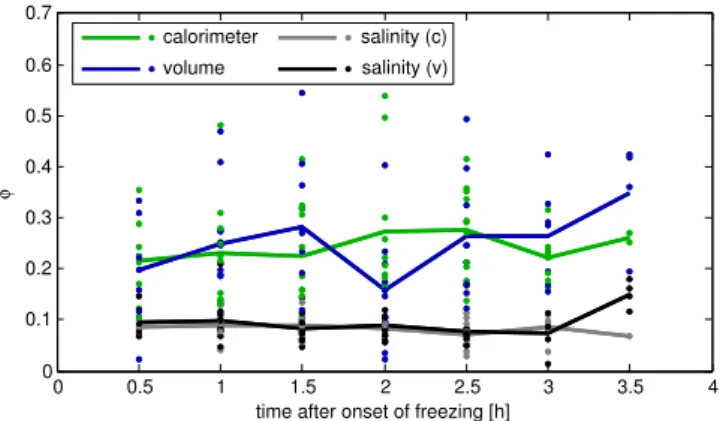
0 0.5 1 1.5 2 2.5 3 3.5 4
0 0.1 0.2 0.3 0.4 0.5 0.6 0.7
time after onset of freezing [h]
φ
calorimeter volume
salinity (c) salinity (v)
Fig. 4.Temporal evolution of the solid fraction from single mea-surements (dots) and as an average over all experiments with waves and with current and wind (lines) analysed with different methods. At each time of measurement two samples were taken, the first one analysed with the calorimeter and the salinity (c) method, the sec-ond one analysed with the volume and the salinity (v) method.
4.1 Methods of solid-fraction measurements
As described in detail in Sect. 2.2, we used three indepen-dent methods to determine the solid fraction of the grease-ice layer. The mean solid fraction as estimated with the salinity method from different samples that were taken at the same time was very similar (Fig. 4), indicating that two samples taken at the same time at slightly different places are compa-rable.
While the mean solid-fraction values from the calorime-ter and the volume method agree very well with each other, the mean values of the solid fraction obtained from the salin-ity method are 50 % lower (Fig. 4). This underestimation is probably due to the assumption made for the salinity method that the salinity of the interstitial water is equal to the salinity of the water under the ice. When ice forms from salt water, salt molecules can not be incorporated into the ice-crystal structure, but will be rejected to the surrounding water. With decreasing temperature of the grease-ice layer, the salinity of the interstitial water increases to maintain phase equilibrium. By fitting the data of Weast (1971), a relationship between the temperature and the salinity of a NaCl solution in phase equilibrium can be described by
S= −0.35471−17.508T−0.33518T2 (5) with a maximum error of 1S=0.005 g kg−1 or 1T =
0.001◦
C in the considered range of salinities from S= 20 g kg−1toS=40 g kg−1or water temperatures fromT =
−1.2◦
C toT = −2.4◦
C. We find vertical mean grease-ice temperatures fromT = −1.8◦
C toT = −2.3◦
C which cor-responds to salinities of the interstitial water betweenS= 30.1 g kg−1andS=38.1 g kg−1(Eq. 5). Unfortunately, the
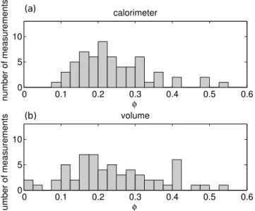
0 0.1 0.2 0.3 0.4 0.5 0.6 0
5 10
calorimeter
φ
number of measurements
0 0.1 0.2 0.3 0.4 0.5 0.6
0 5 10
volume
φ
number of measurements
(a)
(b)
Fig. 5.Histogram of the solid fraction of un-consolidated grease ice for all experiments with waves and with current and wind deter-mined with(a)the calorimeter method and(b)the volume method.
string was not representative for grease ice. However, as-suming interstitial salinity of 35 g kg−1(instead of 29 g kg−1
as in the underlying water) leads to a mean solid fraction of φ=0.25. This is in good agreement with the calorime-ter and the volume method. In a field setup, we suggest to measure the grease-ice surface temperature (e.g. with an IR-thermometer) and assume a linear temperature profile to the grease-ice–water interface to be able to calculate the salinity of the interstitial water with a sea-water equivalent of Eq. (5). In Fig. 5 the distribution of the solid fraction as obtained from the calorimeter method and from the volume method are displayed. The values of the volume method show a wider distribution (standard deviation 0.12) than the values of the calorimeter method (standard deviation 0.10) due to the larger error of the volume method.
4.2 Properties of grease ice
Comparing the results of the three methods discussed above, it is striking that the mean of the solid fraction of the grease-ice layer is not showing a trend in the first 3.5 h (Fig. 4). With values of aboutφ=0.25 for the volume and the calorimeter method, the mean solid fraction is rather constant in time. The same result holds for the individual experiments. Fur-thermore, we do not see a dependence of the solid fraction on the air temperature (not shown). For the calorimeter method, 90 % of the values are betweenφ=0.07 and φ=0.38 and 50 % are betweenφ=0.15 andφ=0.28 (Fig. 5a).
In contrast, the mean of the solid fraction of consol-idated ice directly after its formation from grease ice is
φcons.=0.35 for the experiments with current and wind and φcons.=0.50 for the experiments with waves (not shown).
x
1x
2z
y
2y
12r
α
2r/H
Fig. 6.Sketch of a disc in a cuboid:x1=2r
Hsinα,x2=2rcosα,
y1=2r
Hcosα,y2=2rsinαandz=2r.
The differences in solid fraction of newly consolidated ice in the experiments with current and wind and with waves arise since we always sampled consolidated ice together with the remaining grease underneath. This grease-ice layer was thicker in the experiments with current and wind (see Sect. 3), which is why the vertical mean solid fraction of the newly consolidated ice layer in the experiments with current and wind is lower than in the experiments with waves.
A possible reason for the constant solid fraction of the grease ice before its consolidation is the geometrical pack-ing of the ice crystals in the grease-ice layer. Imaginpack-ing the forming grease-ice layer as randomly oriented ice crystals rising to the surface due to buoyancy, they only occupy a cer-tain part of the volume of the forming grease-ice layer. The emergence of new ice crystals increases the volume of the grease-ice layer but not its solid fraction, leading to a con-stant solid fraction over time in the grease-ice layer as ob-served. Only the consolidation of a grease-ice layer on its surface then leads to an increasing solid fraction, which we also observed.
To get an estimate of the solid fraction of an ice-crystal layer with such randomly oriented ice crystals, we assume for simplicity that the ice crystals are discs with a certain diameter to height ratioH. A disc is put into a cuboid so that it is in contact with the wall. If the disc is lying in parallel to the cuboids base area, the disc takes 78.5 % of the cuboids volume. If the crystal is inclined to form an angleαto the cuboids base area (Fig. 6), the solid fraction is given as
φ= ρi
ρw
π
4H (sinHα+cosα)(cosHα +sinα), (6)
where the factor ρi
ρw accounts for the conversion to a mass
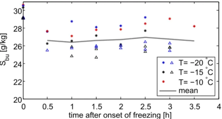
0 0.5 1 1.5 2 2.5 3 3.5 4 20
22 24 26 28 30
time=after=onset=of=freezing=[h] S bu
[g/
kg]
T==−20=°C T==−15=°C T==−10=°C mean
Fig. 7.Temporal evolution of the bulk salinity in the experiments with waves (triangle) and with current and wind (stars) at different air temperatures. The initial salinity for each experiment is indicated at the origin of the time axes.
toα=89◦
) Eq. (6) givesφ=0.22, which is only slightly less than the measured solid fraction and therefore fits our data very well. However, it should be noted that other values for the diameter to height ratio found in literature are in part up to a magnitude higher than the value used here (e.g., Mar-tin and Kauffman, 1981; Weeks and Ackley, 1986), which would lead according to Eq. (6) to estimated solid fractions that are considerably lower thanφ=0.22.
Another explanation for the rather constant solid fraction can be obtained from the so-called mushy-layer equations (see, e.g. Hunke et al., 2011). These equations describe the evolution of general multi-phase, multi-component systems, like sea ice. As long as the Rayleigh number (see Sect. 4.3) is sufficiently small to hinder convective overturning and loss of the salty brine between the ice crystals, and as long as the surface temperature is constant, the mushy-layer equations admit a similarity solution for the solid-fraction distribution within sea ice (e.g. Chiareli and Worster, 1992). Our mea-surements show an almost constant bulk salinity (Fig. 7) and only very small changes of the surface temperature during the first few hours of the experiment. For such constant boundary conditions, and independent of geometrical packing, the sim-ilarity solution of the mushy layer equations predict a con-stant mean solid fraction, with higher solid fraction towards the surface and lower solid fraction towards the ice–ocean interface.
Unfortunately, the vertical resolution of our sampling is too low to allow us to ultimately pin down the constant solid fraction to the geometry argument (which predicts a rather uniform vertical solid-fraction profile) or the similarity so-lution argument (which predicts a vertically varying solid-fraction profile).
The bulk salinity,Sbu, of the grease-ice layer can be
de-termined from the measured salinity of the melted sample, the (volume) ratio of the grease-ice layer to the whole sam-ple and the salinity of the water under the ice layer measured by the uppermost CTD. Values of the calculated bulk salinity
of the grease-ice layer varied betweenSbu=24 g kg−1 and Sbu=29 g kg−1, were independent of air temperature and
al-most constant in time (Fig. 7). The values of the bulk salin-ity in the experiments with current and wind were 1 g kg−1
to 2 g kg−1 higher than the values in the experiments with
waves because the initial salinity of the water was higher in the experiments with current and wind than in the ex-periments with waves. The mean value of the bulk salinity
Sbu=26.5 g kg−1was about 3 g kg−1less than the mean
ini-tial salinity of the water under the ice. 4.3 Properties of nilas
There is very little published data available on the salin-ity evolution of very thin ice. Most data sets (e.g. Cox and Weeks, 1974) only report on the salinity of sea ice with a thickness of more than 10 cm, which is the minimum thick-ness to safely work on sea ice in field conditions. In our lab experiments, however, we are able to estimate the bulk salin-ity,Sbu, of the ice layer from the onset of its formation by
applying salt conservation in the tank based on the measured change in salinity of the water underneath the ice and the ice-thickness evolution. The stratified layer towards the ice– water interface described in Sect. 3 was very thin and could not be substantially more saline than the underlying water for stability reasons. Hence, this layer can be neglected in our calculation.
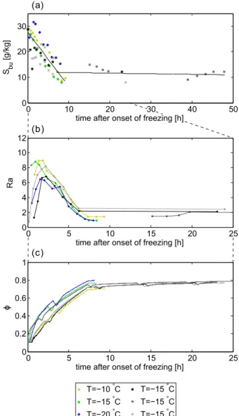
Figure 8a shows the evolution of the bulk salinity in the different quiescent experiments with time and a least square fit to the data. The bulk salinity decreased in all the quies-cent experiments, i.e. independent of air temperature, in the first seven to ten hours from values of 29 g kg−1 to about
10 g kg−1. After ten hours the bulk salinity barely decreased
and stayed relatively constant. The linear least square fit of all values measured in the first ten hours of each experiment gives a decrease of 2.1 g kg−1h−1. We are currently carrying
out a detailed modeling study to further investigate the un-derlying reasons for the rather linear decrease in bulk salinity independent of air temperature in very thin ice.
The rapid decrease of bulk salinity in the first hours of ice formation can be understood by considering the Rayleigh number, Ra. The Rayleigh number is defined as the ratio of available potential energy due to density differences between the brine and the underlying water and the dissipative impact of diffusion and viscosity,
Ra=g(ρw
−ρbr)5h
µκ , (7)
wherehis the ice thickness andg is gravity. The dynamic viscosity of the brine µ and the thermal diffusivity of the brineκare calculated according to the expressions given for sea water by Sharqawy et al. (2010).5is the permeability of the ice layer, which can be approximated as a function of the solid volume fraction,φv, by the empirical relationship5=
10−17(103(1−φ
0 10 20 30 40 50 0
10 20 30
time.after.onset.of.freezing.[h] S bu
[g/
kg]
T=−10.°C T=−15.°C T=−20.°C
T=−15.°C T=−15.°C T=−15.°C
0 5 10 15 20 25
0 0.2 0.4 0.6 0.8 1
time.after.onset.of.freezing.[h]
0 5 10 15 20 25
0 2 4 6 8 10 12
Ra
time.after.onset.of.freezing.[h]
(a)
(b)
(c)
ϕ
Fig. 8.Temporal evolution of(a)the bulk salinity,(b)the Rayleigh number and(c)the solid fraction in the different quiescent experi-ments. The initial salinity for each experiment is indicated in(a)at the origin of the time axes. Color coding of the experiments corre-sponds to the legend at the bottom.
Because the brine temperature determines the salinity of the brine, the density of the brine near the ice surfaceρbrdepends
only on the brine temperature, which was measured with the thermistors.
When the Rayleigh number exceeds a critical value of about Ra=10 (e.g. Worster, 1992; Wettlaufer et al., 1997; Notz and Worster, 2008) convection of brine starts. The bulk salinity then decreases due to gravity drainage, which is the only process that leads to considerable salt loss in sea ice during freezing (Notz and Worster, 2009; Wells et al., 2011). In this study, the maximum of the Rayleigh number at the ice surface was found to be between 7 and 9. This maximum was reached in all experiments within the first 2.5 h after the onset of freezing (Fig. 8b) which corresponds to an ice thickness
of less than 1 cm. Therefore, the early and fast decrease in bulk salinity is in good agreement with the evolution of the Rayleigh number. We do not see a delay in salt release from nilas as measured by Wettlaufer et al. (1997) in a tank ex-periment with a cooling plate in direct contact with the water surface. This difference is caused by the fact that in our ex-periments the surface temperature of the ice evolved freely, causing the initial ice to be relatively warm and hence more permeable than the initial ice in the Wettlaufer et al. (1997) experiments.
Knowing the bulk salinity and the ice temperature, the solid fraction of the ice layer can be calculated. For the bulk salinity, one has Sbu=Siφ+Sbr(1−φ), which gives with Si=0 g kg−1
φ=1−Sbu
Sbr. (8)
The brine salinitySbr=Sbr(Ti)is a function of the ice tem-peratureTi (see Eq. 5) which was measured by the thermis-tors. For calculating the bulk salinity, the fits shown in Fig. 8a are used. Note that Eq. (8) is equivalent to Eq. (2).
The solid fraction increased fast in the first seven hours after the onset of freezing to values ofφ=0.7 to φ=0.8, where low solid fraction corresponds to high air temperature and vice versa (Fig. 8c). This increase in solid fraction is due to the decreasing bulk salinity (because salty brine is draining off the ice layer) and an increasing brine salinity (because ice temperature is decreasing). After seven hours the solid frac-tion stayed almost constant and increased only slightly. The local minima in the solid fraction every sixth hour in Fig. 8c were caused by air temperature variations due to defrosting periods of the cooling system. These periods clearly affected the ice temperature and in this way influenced the solid frac-tion of the ice layer.
4.4 Comparison of properties of grease ice and nilas
Having discussed the bulk salinity and the solid fraction de-velopment with time in the first hours of ice formation for grease ice and nilas separately (Sects. 4.2 and 4.3), these two can now be compared. Finally, we will also discuss the evo-lution of the ice thickness of the two ice types.
4.4.1 Bulk salinity
0 0.5 1 1.5 2 2.5 3 3.5 4 4.5 0
0.2 0.4 0.6 0.8 1
time after onset of freezing [h]
φ
0 0.5 1 1.5 2 2.5 3 3.5 4 4.5
0 0.2 0.4 0.6 0.8 1
time after onset of freezing [h] S bu
/S 0
quiescent exp.
exp. with current and wind exp. with waves
0 5 10 15 20
0 2 4 6 8 10 12
time after onset of freezing [h]
h [cm]
model: ice-free water surface model: closed ice cover (a)
(b)
(c)
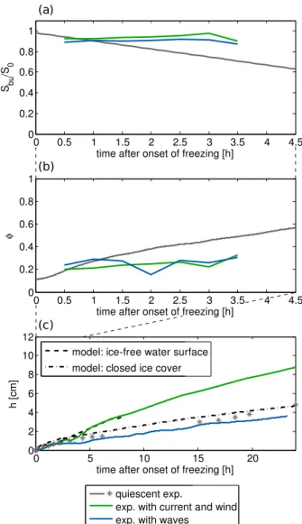
Fig. 9. (a)Temporal evolution of the bulk salinity normalised with the initial salinity of the water as an average over all experiments of each setup.(b)Temporal evolution of the solid fraction as an aver-age over all experiments of each setup. In case of the experiments with waves and with current and wind the values shown are averages of the two reliable methods (calorimeter and volume).(c)Temporal evolution of the measured and modeled ice thickness for experi-ments with different general setup at an air temperature of−15◦C. Color coding of the experiments corresponds to the legend at the bottom.
26.0 psu while their average ocean salinity was 34.5 psu giv-ing a normalised salinity of 0.75.
The bulk salinity of the solid ice layer in the quies-cent experiments began to decrease when convection in the brine channels of the ice layer started. According to the Rayleigh number, convection started at an ice thickness of less than 1 cm and is well described by a linear decrease of 2.1 g kg−1h−1in the first seven hours of freezing. The often
used fit to field data by Cox and Weeks (1974) could not map this early and fast decrease of bulk salinity as the data came
from sea ice that had a thickness of at least 10 cm. However, Cox and Weeks (1974) extrapolated their fit to thinner ice giving a bulk salinity of aboutSbu=14 g kg−1(resembling
a normalised bulk salinity of about 0.5) at an ice thickness of 2 cm, which is in good agreement with our data after the fast, initial decrease.
4.4.2 Solid fraction
Closely linked to the bulk salinity, the solid fraction also de-veloped differently with time in the quiescent experiments compared to the experiments with waves or with current and wind. In Fig. 9b the averages of the solid fraction over all experiments with the same general setup are shown. For the experiments with waves and with current and wind this mean is obtained as the average of the calorimeter and the volume method.
The solid fraction of an ice layer increased with decreasing ice temperature and decreasing bulk salinity. As the ice got thicker with time in the quiescent experiments, the vertically averaged ice temperature decreased, as did the bulk salin-ity (Fig. 8a). Hence, in the quiescent experiments the solid fraction increased from φ=0.10 to φ=0.55 within 4.5 h (Fig. 9b). In contrast to the quiescent experiments, the solid fraction in the grease-ice layer stayed constant in the first 3.5 h with values of aboutφ=0.25 for both the experiments with waves and the experiments with current and wind. This might be due to the geometrical packing of the ice crystals in the grease-ice layer, or be understood in the light of the sim-ilarity solution of the mushy-layer equations (Sect. 4.2). An increased solid fraction of up toφcons.=0.5 was observed for the newly consolidated ice layer in the experiments with waves and with current and wind (not shown), which is com-parable to the solid fraction in the quiescent experiments at the same time (about 4 h after initial ice formation).
The observed values of the solid fraction of the grease-ice layer are in good agreement with other laboratory stud-ies. Martin and Kauffman (1981) measured, depending on the amplitude of their wave field, ice concentrations of up to 40 % by sieving their grease-ice samples. In their work they also mentioned that the sieved grease-ice samples con-sisted of 72 % fresh-water ice and 28 % brine, which trans-lates their concentration to a solid fraction ofφ=0.29. De la Rosa and Maus (2012) measured a solid volume fraction of grease ice in a wave field and stated that grease ice starts to form a consolidated surface at a critical solid volume frac-tion ofφv=0.30. Their critical value corresponds to a solid mass fraction ofφ=0.27 and is therefore also in good agree-ment with the observed mean solid fraction ofφ=0.25 in this study.
when the ice crystals were still kept in suspension by tur-bulence due to waves. We measured ice layer properties in a grease-ice layer almost at rest, as the wave amplitude in our wave experiments was only about 5 cm and the ice crystals accumulated in the ends of the tank to a motionless grease-ice layer in the experiments with current and wind. Within a few hours this grease-ice layer started to form a solid ice layer. Our measurements are therefore not comparable to the early stage measurements of De la Rosa and Maus (2012) or the measurements in the direct proximity to the wave gener-ating paddle of Martin and Kauffman (1981).
Comparing our observed values of the solid fraction of the grease-ice layer with the field measurements of Smed-srud and Skogseth (2006), who measured a mean solid frac-tion of φ=0.25, we find very good agreement. This very good agreement is surprising, since Smedsrud and Skogseth (2006) did not use a correction like that introduced in Sect. 4.1 when applying the salinity method to their sam-ples. Doing so would result in a somewhat larger solid frac-tion, which seems plausible given the higher age and lower normalized bulk salinity of the grease ice in their samples. The probably more vigorous exchange of interstitial water from the grease-ice layer with the underlying sea water in the field compared to our laboratory experiments would result in a smaller correction than we have to apply in this study. A more quantitative estimate of the necessary correction re-mains, however, impossible in the absence of precise temper-ature measurements within the grease-ice layer.
4.4.3 Ice thickness
In addition to the bulk salinity and the solid fraction of the ice layer, the third parameter that describes the ice layer is the ice thickness. In the quiescent experiments the ice thick-ness was read directly from a ruler at the tank wall since the ice thickness was spatially homogeneous in the tank. In the experiments with waves and with current and wind, an av-erage ice thickness has to be estimated indirectly because of the spatially very inhomogeneous ice-layer thickness and a moving ice layer, respectively. Such an estimate of aver-age ice thickness can be obtained from the measured salinity increase in the tank and the known bulk salinity and solid fraction of the ice layer, since the salinity increase in the wa-ter is due to salt release from the forming ice. According to the results in Sect. 4.2, the solid fraction of the ice layer in the experiments with waves and with current and wind is as-sumed to beφ=0.25 in the first two hours. From four hours onwards an ice layer with a consolidated surface dominated. Therefore, the solid fraction is estimated to beφcons.=0.35 in the experiments with current and wind andφcons.=0.5 in the experiments with waves. Between two and four hours af-ter the onset of freezing, a linear increase in solid fraction is assumed.
The resulting (average) ice-thickness development is shown in Fig. 9c. While the ice thickness in the quiescent ex-periments increased about as fast as in the exex-periments with waves, the ice thickness grew about twice as fast in the ex-periments with current and wind. This can be explained by considering the heat flux between the air and the surface, which is higher for open water than in the presence of an isolating ice cover (Maykut, 1982). In the experiments with current and wind, an open water area was maintained rela-tively long by the wind, causing larger heat loss and hence more ice growth in these experiments compared to the quies-cent experiments or the experiments with waves (Sect. 3).
The ice-thickness development in the different experi-ments can be reproduced well with two simple, one dimen-sional models. For ice growth from a closed ice cover, a lin-ear temperature profile in the ice layer with a surface temper-atureT0and a ice–water interface temperature at its freezing pointTf is assumed. For the heat flux through the ice this givesk(Tf−T0)/ h(Stefan, 1889), wherehis the ice thick-ness. The thermal conductivitykiski=2.2 W m−1K−1for
pure ice andkbr=0.5 W m−1K−1 for brine, combining to k=kiφ+kbr(1−φ)for sea ice. If all water is at its freezing point, the heat flux through the ice is equal to the heat that is released due to ice growth,k(Tf−T0)/ h=φρiL(dh)/(dt )
(Stefan, 1889). Integration gives
h(t )=
v u u u t
2
ρiL t
Z
0
k(Tf−T0)
φ dt , (9)
whereφis given according to Eq. (8).
For ice growth from an ice-free water surface, a constant temperature independent of depth is assumed in the grease-ice layer and the underlying water. The heat flux at the grease-ice–air interface is proportional to the difference of the water tem-peratureTw and the air temperatureTa(measured at 12 cm above the ice surface) multiplied with the heat transfer co-efficientC, which is calculated from measurements in the quiescent experiments to beC=20 W m−2K−1. Again this
heat flux is equal to the heat that is released when ice is form-ing, thereforeC(Tw−Ta)=φρiL(dh)/(dt )(Maykut, 1986). Integration gives
h(t )= C
ρiL t
Z
0
Tw−Ta
φ dt, (10)
well with the measured ice thickness in the experiment with current and wind. The grease-ice thickness is only modeled up to seven hours since the solid fraction is not known after-wards. The ice thickness from the model assuming a closed ice cover compares well with the ice thickness in the quies-cent experiments and the experiments with waves.
5 Summary and conclusions
To gain a better understanding of initial sea-ice formation in quiescent and turbulent water, we conducted a tank study in which we simulated the early stages of sea-ice formation under quiescent conditions, in a wave field and under the in-fluence of wind and a current. These experiments allowed us to identify differences and similarities of initial sea-ice for-mation in quiescent and turbulent water. Because of the rel-atively low turbulence that we were able to produce in the tank, in our experiments grease ice only prevailed for a few hours. Our measurements are therefore most closely resem-bling field conditions with rather weak turbulent mixing, as are for example observed in nature once a grease-ice layer has become thick enough to effectively dampen mechanical mixing to greater depth.
We presented new measurements of bulk salinity in very thin sea ice grown from quiescent water, finding that it is well described by a linear decrease in the first hours of ice formation independent of air temperature. In turbulent water, we find that the bulk salinity stayed almost constant as long as grease ice was present.
Measuring the solid fraction of a grease-ice layer, we find that it was constant in the first hours of ice formation with an average value ofφ=0.25, which is in good agreement with geometrical considerations and the work of Martin and Kauffman (1981) and De la Rosa and Maus (2012). From a modeler’s perspective it hence seems sufficient to use a con-stant solid fraction as long as grease ice is present. When the ice layer began to consolidate from the surface, the solid frac-tion started to increase. In contrast to the grease-ice layer, the solid fraction of nilas increased continuously.
We confirm that the development of the ice thickness was primarily influenced by the open water area as the heat flux from the water to the air is larger here than in the presence of a closed ice cover (Maykut, 1982). In our study the ice thickness grew twice as fast in the experiments with current and wind as in the quiescent experiments or the experiments with waves because in the experiments with current and wind an open water area remained at the surface throughout much of the experiment. The evolution of the ice thickness in these experiments could be reproduced well with two simple, one dimensional models.
Additionally, we compared three different methods to calculate the solid fraction from sample measurements in a grease-ice layer. For the salinity method to reveal values which are in agreement with the calorimeter or the
volume method, the salinity of the interstitial water must not be approximated as the salinity of the upper water layer. Instead, the salinity increase of the interstitial water of the grease-ice layer must be taken into account. Because the grease-ice layer has to remain in phase equilibrium, the salinity of the interstitial water of the grease-ice layer is determined by the temperature of the grease-ice layer. Based on the challenge to determine an average grease-ice temperature for the salinity method and the comparatively large error of the volume method, we recommend to use the calorimeter method to measure the solid fraction of a grease-ice layer at least in the laboratory, where immediate sample processing and power supply is no difficulty. For field measurements, we suggest to determine the grease-ice surface temperature and assume a linear temperature profile to the grease-ice–water interface, to be able to obtain reliable results from the salinity method.
Acknowledgements. We thank Iris Ehlert, Lars Henrik Smedsrud,
S¨onke Maus and two anonymous referees for helpful comments that improved this manuscript. We acknowledge financial support through a Max Planck Research Group, the German Academic Exchange Service (DAAD) and the Research Council of Norway.
The service charges for this open access publication have been covered by the Max Planck Society.
Edited by: H. Eicken
References
Anderson, D. L.: Growth rate of sea ice, J. Glaciol., 3, 1170–1172, 1961.
Bromley, L. A., Desaussure, V. A., Clipp, J. C., and Wright, J. S.: Heat capacities of sea water solutions at salinities of 1 to 12 % and temperatures of 2◦C to 80◦C, J. Chem. Eng. Data, 12, 202– 206, doi:10.1021/je60033a013, 1967.
Chiareli, A. O. P. and Worster, M. G.: On measurements and predic-tion of the solid fracpredic-tion within mushy layers, J. Cryst. Growth, 125, 487–494, 1992.
Cox, G. F. N. and Weeks, W. F.: Salinity variations in sea ice, J. Glaciol., 13, 109–120, 1974.
Dai, M., Shen, H. H., Hopkins, M. A., and Ackley, S. F.: Wave raft-ing and the equilibrium pancake ice cover thickness, J. Geophys. Res., 109, C07023, doi:10.1029/2003JC002192, 2004.
De la Rosa, S. and Maus, S.: Laboratory study of frazil ice accu-mulation under wave conditions, The Cryosphere, 6, 173–191, doi:10.5194/tc-6-173-2012, 2012.
De la Rosa, S., Maus, S., and Kern, S.: Thermodynamic investiga-tion of an evolving grease to pancake ice field, Ann. Glaciol., 52, 206–214, 2011.
Fofonoff, P., and Millard Jr, R. C.: Algorithms for computation of fundamental properties of seawater, Unesco Tech. Pap. in Mar. Sci. 44, UNESCO.
Berichte zur Polarforschung 325, Alfred-Wegener Institut f¨ur Polar- und Meeresforschung, Bremerhaven, 1999 (in German). Haas, C., Cottier, F., Smedsrud, L. H., Thomas, D., Buschmann, U.,
Dethleff, D., Gerland, S., Giannelli, V., Hoelemann, J., Tison, J.-L., and Wadhams, P.: Multidisciplinary ice tank study shedding new light on sea ice growth processes, EOS T. Am. Geophys. Un., 80, 507, doi:10.1029/EO080i043p00507-01, 1999. H˚avik, L., Sirevaag, A., Naumann, A. K., and Notz, D.:
Labora-tory study of sea-ice growth and melting: the importance of brine plumes, The Cryosphere Discuss., in preparation, 2012. Hunke, E. C., Notz, D., Turner, A. K., and Vancoppenolle, M.: The
multiphase physics of sea ice: a review for model developers, The Cryosphere, 5, 989–1009, doi:10.5194/tc-5-989-2011, 2011. Lebedev, V. V.: The dependence between growth of ice in Arctic
rivers and seas and negative air temperature (in Russian: rost l’da v arkticheskikh rekakh i moriakh v zavisimosti ot otritsatel’nykh temperatur vozdukha), Problemy arktiki, 5, 9–25, 1938 (cited af-ter Maykut, 1986).
Martin, S.: Frazil ice in rivers and oceans, Ann. Rev. Fluid Mech., 13, 379–397, 1981.
Martin, S. and Kauffman, P.: A field and laboratory study of wave damping by grease ice, J. Glaciol., 27, 283–313, 1981.
Maus, S. and De la Rosa, S.: Salinity and solid fraction of frazil and grease ice, J. Glaciol., 58, 209, doi:10.3189/2012JoG11J110, 2012.
Maykut, G. A.: Large-scale heat exchange and ice production in the Central Arctic, J. Geophys. Res., 87, 7971–7984, 1982. Maykut, G. A.: The surface heat and mass balance, in: The
Geo-physics of Sea Ice, edited by: Untersteiner, N., Plenum Press, New York, 395–463, 1986.
Newyear, K. and Martin, S.: A comparison of theory and laboratory measurements of wave propagation and attenuation in grease ice, J. Geophys. Res., 102, 25091–25099, 1997.
Notz, D.: Thermodynamic and Fluid-Dynamical Processes in Sea Ice, Ph.D. thesis, University of Cambridge, UK, 2005.
Notz, D. and Worster, M. G.: In situ measurements of the evo-lution of young sea ice, J. Geophys. Res., 113, C03001, doi:10.1029/2007JC004333, 2008.
Notz, D. and Worster, M. G.: Desalination processes
of sea ice revisited, J. Geophys. Res., 114, C05006, doi:10.1029/2008JC004885, 2009.
Omstedt, A.: Modelling frazil ice and grease ice formation in the upper layer of the ocean, Cold Reg. Sci. Technol., 11, 87–98, 1985.
Sharqawy, M. H., Lienhard V, J. H. and Zubair, S. M.: Thermophys-ical properties of seawater: A review of existing correlations and data, Desalin. Water Treat., 16, 354–380, 2010.
Shen, H. H., Ackley, S. F., and Yuan, Y.: Limiting di-ameter of pancake ice, J. Geophys. Res., 109, C12035, doi:10.1029/2003JC0021232004, 2004.
Smedsrud, L. H.: Frazil-ice entrainment of sediment: large-tank lab-oratory experiments, J. Glaciol., 47, 461–471, 2001.
Smedsrud, L. H.: Grease-ice thickness parameterization, Ann. Glaciol., 52(57), 77–82, 2011.
Smedsrud, L. H. and Skogseth, R.: Field measurements of Arctic grease ice properties and processes, Cold Reg. Sci. Technol., 44, 171–183, 2006.
Stefan, J.: ¨Uber die Theorie der Eisbildung, insbesondere ¨uber die Eisbildung im Polarmeere, Sb. Kais. Akad. Wiss., Wien, Math.-Naturwiss., 98, 965–983, 1889 (in German).
Weast, R. C.: Handbook of Chemistry and Physics, 52th Edn., Chemical Rubber Co., Cleveland, OH, 1971.
Weeks, W. F. and Ackley, S. F.: The growth, structure, and prop-erties of sea ice, in: Geophysics of Sea Ice, edited by: Unter-steiner, N., Plenum Press, New York, 9–164, 1986.
Wells, A. J., Wettlaufer, J. S., and Orszag, S. A.: Brine fluxes from growing sea ice, Geophys. Res. Lett., 38, L04501, doi:10.1029/2010GL046288, 2011.
Wettlaufer, J. S., Worster, M. G., and Huppert, H. E.: Natural con-vection during solidification of an alloy from above with appli-cation to the evolution of sea ice, J. Fluid Mech., 344, 291–316, 1997.
Wilkinson, J. P., DeCarolis, G., Ehlert, I., Notz, D., Evers, K.-U., Jochmann, P., Gerland, S., Nicolaus, M., Hughes, N., Kern, S., De la Rosa, S., Smedsrud, L., Sakai, S., Shen, H., and Wad-hams, P.: Ice tank experiments highlight changes in sea ice types, EOS T. Am. Geophys. Un., 90, 81–82, 2009.