Computer Simulation of the Stochastic Dynamics of Super-Paramagnetic
Particles in Ferrofluids
Claudio Scherer
Institute of Physics, Federal University of Rio Grande do Sul, Porto Alegre, Brazil
Received on 7 September, 2005
Several papers have been written on the complex problem of the stochastic dynamics of the magnetic moments of super-paramagnetic particles, simultaneously with the stochastic rotation of these colloidal particles in a ferrofluid [1–3]. None of these works, however, is sufficiently general and conveniently simple and clear to be used in sumulational works to appropriately describe the experimental super-paramagntetic resonance lines. We have a new proposal for the equations of rotational motion, which is appropriate for simulations. Those equations are stochastic differential equations with multiplicative noise. Therefore, they have to be interpreted as Stratonovich-Langevin equations and the roles of stochastic calculus have to be used in the simulations. For this reason we will briefly present the essence of the numerical algorithms used in the solutions of Stratonovich equations. Finally, the simulational results for the magnetic response functions, and the corresponding dynamic susceptibilities, will be shown and their consequences will be analyzed.
Keywords: Ferrofluid, Magnetic fluid; Computer simulation; Stochastic dynamic; Super-paramagnetic
I. INTRODUCTION
The dynamics of the magnetic moments of super-paramagnetic particles constitute a nice example of problem in the Physics of condensed matter where to apply the tools of stochastic calculus to perform numerical simulation. If those particles are in a ferrofluid, then the problem becomes still more interesting, because one has a coupled rotational motion of the moments with respect to the particles and of the particles with respect to the fluid. Several physical vari-ables may be calculated from the numerical solutions of the equations of motion for an ensemble of super-paramagnetic particles, which can then be compared to experimental re-sults. We give particular attention to the linear response func-tions, from which the dynamical susceptibility is obtained by Fourier transform, and then the magnetic resonance absorp-tion lines.
In section II we introduce some hypothesis, which are very realistic for real ferrofluids, defining in this way the essence of the model. The equations of motion are also introduced in this section. Since the simulation is done for an equilib-rium ensemble of particles, the probability distributions of the relevant variables is discussed in section III. General prop-erties of stochastic differential equations and numerical pro-cedures to get solutions for their realizations are treated in section IV. Finally, in section V we solve the set of equa-tions for the super-paramagnetic particles, for different values of the physical parameters, calculate the response functions and the corresponding dynamical susceptibilities and present the results in figures. Some consequences of our results are discussed.
II. THE MODEL AND THE EQUATIONS OF MOTION
Some hypothesis used in this work are:
1) The magnetic particle has a symmetry axis of easy mag-netization, which will be characterized by the unit vectorc;
2) The particle’s magnetic momentµhas constant modulus µand can rotate inside the particle under the influence of an interaction potential modeled byV=−K(µ·c)2, whereKis a constant, called ”anisotropy constant”; we will use units such thatµ=1;
3) The particle’s rotational inertia is negligible in the equa-tions of motion, in comparison with the Brownian and dissi-pative terms;
These three hypothesis are very realistic for the normal con-ditions of super-paramagnetic particles in ferrofluids above the blocking temperature.
The equations of motion forµare obtained from the classi-cal equation for the rotation of a system with angular momen-tumJin presence of a torqueN,
dJ
dt =N. (1)
The existence of a magnetic momentµimplies the existence of an angular momentum, such thatµ=gJ. In the general case the ”gyromagnetic factor”g is a tensor, but frequently it is simply a scalar. We will assume this to be the case and chose units such thatg=1. Therefore Eq.(1) may be written as
dµ
dt =N (2)
The torques onµare:
a) The torque due to the interaction potentialV of hypothe-sis 2 above is obtained by derivingVwith respect to the angle betweenµandc, which results in 2K(µ·c)(µ×c);
b) The Brownian torque due to the atomic vibrations of thermal origin (phonons) of the particle:αµµ×ξµ;
c) The dissipative torque of resistance to the Brownian ro-tation (fluctuation dissipation theorem):−γµµ×µ˙(throughout
d) The torque of interaction ofµ with a magnetic fieldH, applied or due to the other particles in the ferrofluid, which happens to be present at the particles position:µ×H.
Therefore the equation of motion forµ, Eq.(2), may be writ-ten as
dµ dt =µ×
n
H+2K(µ·c)c−γµ
dµ dt +αµξµ
o
(3)
Substituting ddtµ at the RHS of Eq.(3) by the whole of the RHS, and using the properties of the triple vector product we get
dµ dt =
1 1+γ2
µ
µ×nH+2K(µ·c)c+αµξµ−γµµ× {H+2K(µ·c)c+αµξµ}
o
(4)
If we callHe f f =H+2K(µ·c)c+αµξµ, Eq.(4) becomes the
equation of Landau-Lifshitz.
The only motion of the particle which will be considered is the rotation of the symmetry axis,c, since the rotation around cis irrelevant for the motion of µ. The last three terms of Eq.(3) are due to the interaction of µ with the particle and, therefore, they have to be present, with opposite sign, in the equation for c. Besides those terms there is the Brownian torque on the particle, due to the thermal motion of the liquid’s molecules and the corresponding dissipative torque, according to the fluctuation-dissipation theorem. Since the rotational in-ertia of the particle will be neglected (hypothesis 3 above), the equation of motion forcreduces to a balance between the torques,
−2K(µ·c)(µ×c)+γµµ×µ˙−αµµ×ξµ−γlc×c˙+αlc×ξl=0,
(5) which may be written more conveniently as
γlc×c˙=−2K(µ·c)(µ×c) +γµµ×µ˙−αµµ×ξµ+αlc×ξl.
(6) Making the vector product of Eq.(6), at the left, bycand using the properties of the triple vector product, follows
dc dt =
c γl×
n
µ×£2K(µ·c)c−γµ
dµ dt +αµξµ
¤
+αlξl
o
, (7)
where, in the last term, we substitutedc×(c×ξl)byc×ξl,
because both expressions are white noise perpendicular toc and, therefore, have the same statistical properties and the last expression is simpler.
III. EQUILIBRIUM DISTRIBUTIONS
Before performing the simulations of the dynamics ofµand cwe need to get the equilibrium distributions of these vectors, which are the initial distributions from which we will simulate the dynamics. The independent stochastic variables are the
polar coordinatesθandφofµand the polar coordinatesϑand
ϕofc.
The equilibrium distribution for these four independent variables, in presence of a magnetic fieldHin thezdirection, is given by Boltzmann’s distribution,
Po(θ,φ,ϑ,ϕ) =Csin(θ)sin(ϑ)exp((K(µ·c)2+µ·H)/T) (8) whereµ·c=sinθsinϑcos(φ−ϕ) +cos(θ)cos(ϑ), µ·H=
Hcos(θ)
andCis a normalization constant.
To obtain, the equilibrium distribution for one of the vari-ables, for examplePo(θ), forθ, we perform the numerical
integration of the other independent variables,φ,ϑandϕ(see Fig.1, lines a and b).
For the simulation of the dynamics we will need to gen-erate an equilibrium ensemble of particles with coordinates distributed according to Eq.(8). There are several ways of doing this [4, 5]. Fig.1, line c, showsPo(θ)obtained form the histogram for theθ’s of 10000 particles of an equilibrium ensemble, for different parameters, as described in the figure caption. When the histogram is done for 1000000 particles, as in the dynamic simulation described below, the theoretical and simulated curves become indistinguishable.
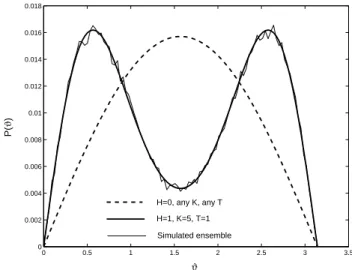
It is interesting to note that the equilibrium distribution of the orientation ofµ is independent of the anisotropyK. The orientation ofµdepends on the ratioH/T while the orienta-tion of the particle, specified byc, depends onH,KandT, as can be seen in Fig.2.
We will see bellow that for the dynamic response of the magnetization this independence of the orientation ofµwith respect to the anisotropy does not happen, i.e., the dynamic behavior ofµdepends on the anisotropy.
IV. NUMERICAL SIMULATION OF STOCHASTIC DIFFERENTIAL EQUATIONS WITH MULTIPLICATIVE
NOISE
0 0.5 1 1.5 2 2.5 3 3.5 0
0.005 0.01 0.015 0.02 0.025
θ
P(
θ
)
H=0, any T
H=1, T=1, any K a)
b)
c) H=1, T=1, any Kby simulation
FIG. 1: Equilibrium distribution for the angleθbetweenµandH: a) without applied field; b) with fieldH=1, parallel to thez-axis; c) line plot of a histogram for the computer generation of the independent coordinates for 10000 particles with probability distribution given by Eq.(8)with fieldH=1; all curves are independent of the value of the anisotropyK.
0 0.5 1 1.5 2 2.5 3 3.5
0 0.002 0.004 0.006 0.008 0.01 0.012 0.014 0.016 0.018
P(
ϑ
)
ϑ
H=0, any K, any T
H=1, K=5, T=1 Simulated ensemble
FIG. 2: Equilibrium distribution for the angleϑbetweencandH. Dashed line: without applied field, it is just a sin(ϑ); solid thick line: with fieldH=1, parallel to thez-axis,K=5 andT=1; solid thin line: plot of a histogram for the computer generation of the inde-pendent coordinates for 10000 particles with probability distribution given by Eq.(8) with the same parameters as in the thick line.
dX(t) =A(X)dt+B˜(X)dW(t) (9) whereX(t)is an n-component vector (in our case n=6, X = [µ,c] = [µx,µy,µz,cx,cy,cz]), A(X) is an n-component
vector (RHS of equations 4 and 7, except for the terms with the white-noise),dW(t)is an m-component ”Wiener differen-tial” (see reference [6]), which corresponds to the integral of the white-noise over the time interval (t,t+dt), and ˜B(X)is
ann×mmatrix. Each componentdWj ofdW is a Gaussian
stochastic process with zero mean and variancedt, i.e.,
dWj(t)
®
=0
dWj(t)dWk(t)
®
=δj,kdt. (10)
In some cases ˜Bis a constant matrix, i.e., does not depend onX, and then Eq.(9) is said to be of ”additive noise”. Oth-erwise, namely when ˜Bdepends onX, the equation is said to be of ”multiplicative noise”. In the former case Eq.(9) may be solved by ”ordinary stochastic calculus”, while in the last case one have to use ”Stratonovich” or ”Ito” calculus. This is the case of equations (4) and (7), since ˜Bcontains vector products withµandc, which are components ofX.
We write Eq.(9) in terms of ”finite differences”, according to Stratonovich calculus. Calling∆t, ∆X and∆W the finite differences oft,XandW between two consecutive instants of the discretized time, we have
∆X=A(X+∆X/2)∆t+B˜(X+∆X/2)∆W (11) The term∆X/2 in the argument ˜Bessential for Stratonovich calculus, whereas it is optional, but convenient, in the argu-ment ofA.
To generate, in computer simulation, the independent com-ponents∆Wj of the ”Wiener increments”∆W, we proceed in
the following way: generate a Gaussian random numberRG,
with zero mean and unit variance and write
∆Wj=
√
∆t RG (12)
since the width of the distribution for∆Wjis
√
∆t.
It is in general, and in our case in particular, difficult, or even impossible, to isolate ∆X in Eq.(11). For this reason we will use an algorithm which we call “second order Stratonovich”, as follows:
1) Calculate∆X0equal to the RHS of Eq.(11) without the terms∆X/2 in the arguments ofAand ˜B;
2) Use∆X0instead of∆X in the arguments ofAand ˜Bto obtain∆X.
This procedure is analogous to Runge-Kutta 2ndorder in the case of ordinary differential equations. It gives the same level of precision as we would have by transforming Eq.(9) into an Ito differential equation and integrating it by Ito calculus, but it is simpler to implement.
V. SOLUTION OF EQUATIONS (4) AND (7) BY STRATONOVICH CALCULUS
dµ = 1
1+γ2
µ
µ×nH+2K(µ·c)c−γµµ× {H+2K(µ·c)c}
o dt+
+ αµ
1+γ2
µ
µ×ndWµ−γµµ×dWµ
o
(13)
dc= c
γl×
n µ×£
2K(µ·c)c dt−γµdµ¤+αµµ×dWµ+αldWl
o
(14) Now we write equations (13) and (14) in form of finite differences according to Stratonovich integration rule. For the time step(t,t+∆t)we use the following notation:µ=µ(t);c=c(t); and∆µand∆cthe corresponding increments in the interval.
∆µ = 1
1+γ2
µ
(µ+∆µ/2)× ½
H+2K³(µ+∆µ/2)·(c+∆c/2)´(c+∆c/2)
− γµ(µ+∆µ/2)×
n
H+2K³(µ+∆µ/2)·(c+∆c/2)´(c+∆c/2)o
¾ dt+
+ αµ
1+γ2
µ
(µ+∆µ/2)× ½
dWµ−γµ(µ+∆µ/2)×dWµ
¾
(15)
∆c = c+∆c/2
γl ×
½
(µ+∆µ/2)×h2K³(µ+∆µ/2)·(c+∆c/2)´(c+∆c/2)dt
− γµ∆µ
i
+αµ(µ+∆µ/2)×dWµ+αldWl
¾
(16)
We obtainµ(t+∆t)andc(t+∆t)proceeding as follows, ac-cording to the 2nd order Stratonovich algorithm, as described in section IV:
1) Calculate∆µ0from Eq.(15), by neglecting everywhere at the RHS the terms∆µ/2 and∆c/2;
2) Calculate∆c0from Eq.(16), by neglecting everywhere at the RHS the terms∆µ/2 and∆c/2 and using∆µ0, just calcu-lated, instead of∆µin the termγµ∆µ;
3) Calculate∆µ from Eq.(15), by using∆µ0/2 and∆c0/2 everywhere at the RHS instead of∆µ/2 and∆c/2;
4) Calculate∆cfrom Eq.(16), by using∆µ0/2 and ∆c0/2 everywhere at the RHS instead of∆µ/2 and∆c/2 and using
∆µ, just calculated, in the termγµ∆µ;
5) Obtainµ(t+∆t) =µ+∆µandc(t+∆t) =c+∆cand cor-rect the norms of those quantities from the small errors (2nd
order in∆t), which may be produced by the above calcula-tions, by dividing both by their corresponding norms.
VI. LINEAR RESPONSE FUNCTIONS AND DYNAMIC SUSCEPTIBILITIES
Assume that a weak fieldF(t)is applied on a system and an observable variableB(t)changes its expectation value from the equilibrium valueB0to
B(t)®
=B0+δB(t), whereδB(t)
is a linear functional ofF(t). Assume also that, as is usually the case, the interaction energy ofF with the system may be
written in the form
H
(t) =−A(t)F(t), whereA(t)is a dy-namical variable of the system. The linear response functionΦBAis implicitly defined by
δB(t) =
Zt
−∞ΦBA(
t−t′)F(t′)dt′. (17)
Assuming, for simplicity, that the equilibrium valuesA0and B0are zero, the ”Kubo formula” (see equation 4.2.20 of refer-ence [7]), which relates the correlation function ofAandBto
ΦBA, in the classical case, may be written as
ΦBA(t) =
½
−β˙
B(t)A(0)®
fort≥0
0 fort<0 (18) whereβ=1/kBT and···®means average over an
equilib-rium distribution for a canonical ensemble of systems. In the case of a magnetic fieldHi(t), applied in directioni,
the response functionΦji of the magnetization in direction j
is
Φji(t) =µ˙j(t)µi(0)® fort≥0. (19)
evolution ofµj(t)as explained in section V, makes the
prod-uct ˙µj(t)µi(0) for each particle, sums over all particles and
divides byN.
In what follows we apply the above ”recipe” to calculate the magnetic response functions of the super-paramagnetic par-ticles in ferrofluids, for several sets of material parameters. From the response functions, by Fourier transform, we obtain the corresponding dynamic susceptibilities,
χ(ω) =χ′(ω) +iχ′′(ω) =
Z ∞
0 Φ(
t)exp(−iωt)dt. (20) The absorption power in magnetic resonance is propor-tional to the imaginary part of the susceptibility,
P(ω)∝ ωχ′′(ω), (21) which makes the susceptibility a very important function.
We chose a set of values for the material parameters, in adimensional units, as our standard. Then, by varying one parameter in each calculation, we isolate its effect on the dy-namics. For our standard we chose:
H=1, K=1, γµ=0.01, γl=1, T=1; (22)
Figure 3 shows the results of the calculations for the re-sponse functionsΦxx(t)andΦyx(t), for the case of the
stan-dard values of the parameters. We used an ensemble of 1000000 particles.
0 5 10 15 20 25 30 35 40
−0.3 −0.2 −0.1 0 0.1 0.2 0.3 0.4
time
Φ
(t)
γµ=0.01
γ
l=1.0 K=1.0 H=1.0 T=1.0 Standard values
Φ
xx (t)
Φ
yx(t)
FIG. 3: Response functionΦxx(t)(full line) andΦyx(t)(dashed line) for the standard case, with parameter values as written on the inset.
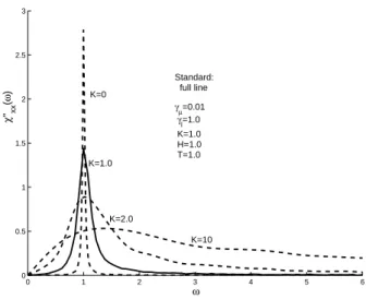
Figure 4 shows the imaginary part of the susceptibil-ity, χ′′xx(ω), for the standard case and several values of the
anisotropy, keeping the standard values for the other parame-ters. One sees that in absence of anisotropy there is a very narrow, well pronounced, resonance line, while for increasing
0 1 2 3 4 5 6
0 0.5 1 1.5 2 2.5 3
Standard: full line
γµ=0.01
γl=1.0 K=1.0 H=1.0 T=1.0
ω
χ
"xx
(
ω
) K=0
K=1.0
K=2.0
K=10
FIG. 4: Imaginary part of the susceptibility,χ′′xx(ω)for the standard case (full line), and several values of the anisotropy (dashed lines, as indicated), keeping the standard values for the other parameters.
anisotropy the resonance becomes broader and less well pro-nounced. For very high K, which corresponds to ”blocked” magnetic moment, the resonance disappears.
Figure 5 shows the effect of both viscosities on the suscep-tibility. The doted and dashed lines correspond to increaseγµ
andγl, respectively, by a factor of 10. One sees that in both
cases the line becomes broader, less intense and centered on a slightly higher resonance frequency.
0 1 2 3 4 5 6
0 0.5 1 1.5
ω
χ
,,(xx
ω
)
γµ = 0.01, γ l =1.0
γµ = 0.1, γl = 1.0
γµ = 0.01, γl = 10.0
FIG. 5: Imaginary part of the susceptibility,χ′′
xx(ω), for higher vis-cosities,γµ=0.1 (dotted line) andγl=10 (dashed line), compared to the case of the standard values (full line).
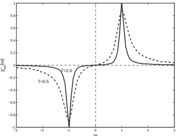
−3 −2 −1 0 1 2 3 −1
−0.8 −0.6 −0.4 −0.2 0 0.2 0.4 0.6 0.8 1
ω
χ
,,(xx
ω
)
T=2.0
T=0.5
FIG. 6: Imaginary part of the susceptibility corresponding to diferent temperatures, T=2 (full line) and T=0.5 (dashed line).
VII. CONCLUSIONS
In conclusion one can say that:
1) Simulation of the dynamics of super-paramagnetic mo-ments in ferrofluids, when compared to resonance experi-ments, can give important information about their properties:
a) Bigger K: broader resonance line, same resonance fre-quency;
b) Very big K (blocked): no resonance;
c) Biggerγµ or γl : broader resonance line and slightly
higher resonance frequency;
d) Higher temperature: narrower line, same resonance fre-quency;
2) Second order Stratonovich is a very good algorithm to sim-ulate realizations of the dynamics of super-paramagnetic mo-ments in ferrofluids.
[1] M.I. Shliomis and V.I. Stepanov, Adv. Chem. Phys.87, 1 (1994). [2] C. Scherer and H. G. Matuttis, Phys. Rev. E63, 0115504 (2001). [3] C. Scherer and T. F. Ricci Braz. J. Phys.31, 380 (2001). [4] W.H. Press et. al., Numerical Recipies, Cambridge University
Press, New York, 1992
[5] C. Scherer,M´etodos Computacionais da F´ısica, ed. Livraria da F´ısica, Universidade de S˜ao Paulo (2005);
[6] C.W. Gardiner, Handbook of Stochastic Methods for Physics,
Chemistry and Natural Sciences, Springer-Verlag, Berlin, 1999;
[7] R. Kubo, M. Toda and N. Hashitsume, Statistical Physics II:
Nonequilibrium Statistical Mechanics, Springer-Verlag, Berlin,