Study on the limitations of traveltime inversion in the presence of extreme velocity anomalies

(1)

SED

5, 189–226, 2013

Limitations of traveltime inversion

and high velocity contrasts

I. Flecha et al.

Title Page

Abstract Introduction

Conclusions References

Tables Figures

◭ ◮

Back Close

Full Screen / Esc

Printer-friendly Version Interactive Discussion

Discussion

P

a

per

|

Dis

cussion

P

a

per

|

Discussion

P

a

per

|

Discussio

n

P

a

per

|

Solid Earth Discuss., 5, 189–226, 2013 www.solid-earth-discuss.net/5/189/2013/ doi:10.5194/sed-5-189-2013

Geoscientiic Geoscientiic

Open Access

Solid Earth

Discussions

This discussion paper is/has been under review for the journal Solid Earth (SE). Please refer to the corresponding final paper in SE if available.

Study on the limitations of traveltime

inversion in the presence of extreme

velocity anomalies

I. Flecha1, R. Carbonell1, and R. W. Hobbs2

1

Estructura i Din àmica de la Terra, Institut de Ci ències de la Terra “Jaume Almera”-CSIC, C/ Llu´ıs Sol é i Sabar´ıs s/n, 08028, Barcelona, Spain

2

Department of Earth Sciences, University of Durham, Durham DH1 3LE, UK

Received: 12 February 2013 – Accepted: 13 February 2013 – Published: 20 March 2013

Correspondence to: R. Carbonell (ramon.carbonell@csic.es)

(2)

SED

5, 189–226, 2013

I. Flecha et al.

Title Page

Tables Figures

◭ ◮

Back Close

Full Screen / Esc

Discussion

P

a

per

|

Dis

cussion

P

a

per

|

Discussion

P

a

per

|

Discussio

n

P

a

per

Abstract

The difficulties of seismic imaging beneath high velocity structures are widely recog-nised. In this setting, theoretical analysis of synthetic wide-angle seismic reflection data indicates that velocity models are not well constrained. A two-dimensional velocity model was built to simulate a simplified structural geometry given by a basaltic wedge

5

placed within a sedimentary sequence. This model reproduces the geological setting in areas of special interest for the oil industry as the Faroe-Shetland Basin. A wide-angle synthetic dataset was calculated on this model using an elastic finite difference scheme. This dataset provided travel times for tomographic inversions. Results show that the original model can not be completely resolved without considering additional

10

information. The resolution of nonlinear inversions lacks a functional mathematical re-lationship, therefore, statistical approaches are required. Stochastical tests based on Metropolis techniques support the need of additional information to properly resolve subbasalt structures.

1 Introduction

15

Subsalt and subbasalt imaging has been a key objective during the last 2 decades for the oil exploration (Rousseau et al., 2003; Williamson, 2003; Sava and Biondi, 2004). Oil exploration has revealed the imaging difficulties in the presence of high velocity features (such as salt and/or basalts). Low velocity structures under relatively high velocity features are poorly constrained by conventional processing and/or inversion

20

schemes (Flecha et al., 2004). Velocity provides the link between seismic images and rock types. Ray tracing theory, based on Fermat’s principle, states that regions sur-rounded by higher velocities are undersampled by rays. Seismic images of the subsur-face strongly benefit from well resolved estimation of seismic velocities. These seismic velocities are currently determined by velocity analysis and, in the best case, by travel

25

(3)

SED

5, 189–226, 2013

I. Flecha et al.

Title Page

Tables Figures

◭ ◮

Back Close

Full Screen / Esc

Discussion

P

a

per

|

Dis

cussion

P

a

per

|

Discussion

P

a

per

|

Discussio

n

P

a

per

|

reflection/refraction shotgathers (Zelt and Smith, 1992). The determination of the ve-locity models requires the interpretation/identification of the seismic arrivals within a shotgather. Furthermore, the mathematical inversion schemes require digitized travel times, offset pairs, to calculate velocities. Usually, a standard crustal velocity model features an increasing velocity in depth, however in the presence of salt and/or basaltic

5

intrusions this assumption fails. Intrusions often represent the emplacement of a high velocity body in the crust, therefore zones beneath these structures may feature low velocities. This is the case of basalt covered areas as erupted basalt buries previous structures that may feature low velocities such as in the Faroe Shelf. In the Faroe Shelf, covered areas represent potential hydrocarbon reservoirs, therefore this topic is of

spe-10

cial interest for the industry.

This manuscript developes a theoretical study investigating the reliability and efec-tiveness of travel time inversion of wide-angle seismic reflection/refraction data. We investigated when and to what extent the low velocity structure beneath a high velocity basalt layer can be resolved.

15

2 Geological setting and imaging problems

In the Faroe-Shetland Basin, Mesozoic and Tertiary sedimentary sequences fill the basin but, close to the Faroe Shelf, these sedimentary sequences are covered by Paleocene-Eocene basaltic lavas of which the Faroe Islands are composed. The pre-vious topography of the basin was dominated by normal faults as a consequence of

20

the extension and subsidence during Cretaceous and Paleocene (Richardson et al., 1999). As huge amounts of molten rock were extruded, after filling the lows between fault blocks, lava flows extended over long distances in the basin. Basalt flows were erupted in several episodes and three major units have been identified: Lower, Mid-dle and Upper Series. The composition and thickness differs from one unit to another.

25

(4)

SED

5, 189–226, 2013

I. Flecha et al.

Title Page

Tables Figures

◭ ◮

Back Close

Full Screen / Esc

Discussion

P

a

per

|

Dis

cussion

P

a

per

|

Discussion

P

a

per

|

Discussio

n

P

a

per

In the Faroe Shelf, geologic and geophysical data suggest that a layer of basalt is placed within two low velocity sedimentary sequences (Hughes et al., 1998; Richard-son et al., 1998, 1999; Fliedner and White, 2003; Smallwood et al., 2001; Sørensen, 2003; White et al., 2003; Raum et al., 2005). The velocity structure for sediments above the basalt can be resolved by conventional techniques. The top of the basalt layer can

5

be determined very effectively due to the high contrast in seismic physical properties between the basalt and the overlying sediments. However, the high velocity basalt layer represents a complex scenario for seismic imaging methodologies, acting as a barrier so that the underlying structures can not be imaged. The high velocity that character-izes the basalt constrasts with relatively low velocity of the surrounding materials. This

10

causes that most of energy is reflected and/or travels along this layer.

Although basalt flows tend to be subhorizontal on large scale, at small scale, rugged interfaces cause scattering and disperse the elastic energy destroying any lateral co-herency of possible subbasalt events. In addition to the di_fferences between the three major Series, within every unit, basaltic bodies are highly heterogeneous in

compo-15

sition and physical properties. These heterogeneities strongly disperse the seismic energy and destroy the signal coherence in the seismic wavefield. The outter parts of the basalt flows are affected by weathering causing a decrease in velocity, this con-strasts with the internal parts which cooled slowly and without any external influence preserving a high velocity feature. Interfaces between individual flows in a basalt block

20

produce internal multiples and wave conversions. Also some intrusive basalt flows were emplaced as sills within previous structures providing an additional cause for scattering at and beneath the base of the basalt.

In addition to these major imaging issues, the usual problems of marine seismic reflection data acquisition must be also considered (tidal noise, multiples, peg-leg,

re-25

(5)

SED

5, 189–226, 2013

I. Flecha et al.

Title Page

Tables Figures

◭ ◮

Back Close

Full Screen / Esc

Discussion

P

a

per

|

Dis

cussion

P

a

per

|

Discussion

P

a

per

|

Discussio

n

P

a

per

|

et al., 1999; White et al., 2002; Ziolkowski et al., 2003), understanding the scattering caused by the basalt (Martini et al., 2001; Martini and Bean, 2002) or combining several geophysical methodologies (Jegen-Kulcsar and Hobbs, 2005). Nevertheless, studying subbasalt structures requires a detailed velocity model to obtain valuable information and to apply more sophisticated approaches such as prestack depth migration.

5

3 Theoretical geologic model and synthetic seismic data

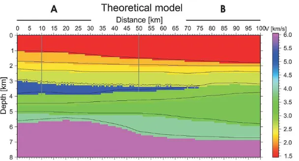
A synthetic dataset was acquired using an idealized velocity model. The model consists of a wedge of basalt layer within a sedimentary column. The basalt layer features an irregular upper surface, and very high velocities and densities that contrast with the velocities and densities of the surrounding sediments. The choice of a thin wedge for

10

the basalt is justified because it represents the best geological setting for exploration and explotation for the oil industry. In order to simulate a highly variable structure, we consider the small-scale top basalt topography to be a random field which was generated using Von Karman functions (Go_ff and Jordan, 1988). As there is a high velocity contrast between the sedimentary cover and the basalt, can this topography

15

be recovered? In addition, in the case of Shetland-Faroe Basin, the area where the basalt thins is close to the center of the basin where geology is well known and can be extrapolated to suggest the existence of subbasalt sedimentary structures. The P-wave velocities were taken from laboratory measurements (Carmichael, 1982). All the physical properties used in the simulation are summarized in table 1.

20

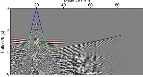
A second order finite difference solver of the elastic wave equation using Sochacki’s interface scheme (Sochacki et al., 1987, 1991) was used to generate a seismic dataset acquired over the velocity model. The 2-D model was of 100 km wide and 8 km deep and a 10×10 m grid was used (Fig. 1). After intense calculations, 80 shotgathers were simulated with more than 3000 traces per shot (one trace every 30 m) and 30 s of

25

(6)

SED

5, 189–226, 2013

I. Flecha et al.

Title Page

Tables Figures

◭ ◮

Back Close

Full Screen / Esc

Discussion

P

a

per

|

Dis

cussion

P

a

per

|

Discussion

P

a

per

|

Discussio

n

P

a

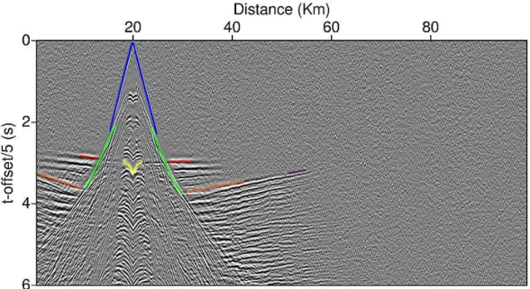
per

these simulations are summarized in table 2. In this data several phases were identified (Fig. 2).

Water multiple and peg-leg signal were generated by the elastic finite difference al-gorithm, no additional noise was included in the data. Although in nature, basalts ap-pear as highly heterogeneous layered structures, in order to simplify the problem, the

5

basaltic wedge was considered as an homogeneus feature in its internal velocity distri-bution. Under these conditions we obtained a quite ideal dataset.

4 Tomographic inversions

The main aim of synthetic simulations was checking the possibility of recovering the original model using tomographic techniques. As a first attempt, first arrivals travel

10

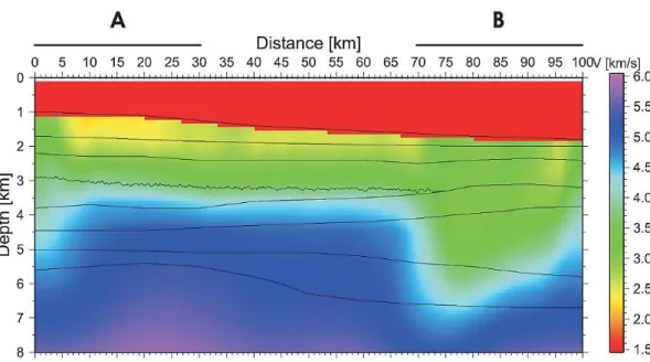
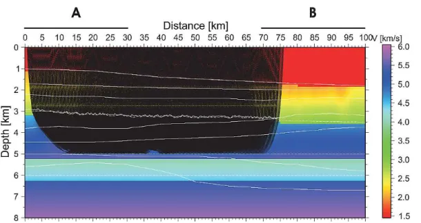
time seismic tomography was applied using the TTT software package (Trinks et al., 2005). This code is based on initial value ray tracing in velocity models constructed of Delaunay triangulated grids and interfaces. The tomography is implemented as a joint interface and velocity inversion using the bi-conjugated gradient method, for further details see Trinks (2003). The result obtained for this inversion is shown in Fig. 3. The

15

average velocity structure of the zone over the basalt layer was recovered as well as the top of the basalt layer where a sharp velocity contrast is displayed. However, no low velocity can be reproduced under the basalt, toward the right end of the model, where no basalt exists, some realistic information about velocities can be obtained for the deepest part of the model. These results suggest that there are physical limitations

20

in constraining subbasalt structures by seismic travel time tomography.

TTT code can also invert additional phases. In order to include all the informa-tion from phases identified in synthetic shots, a layer by layer striping inversion was performed and develloped in detail in what follows. A five layer model was used as starting model: water, sediments (over basalt), basalt, sediments (under basalt) and

25

(7)

SED

5, 189–226, 2013

I. Flecha et al.

Title Page

Tables Figures

◭ ◮

Back Close

Full Screen / Esc

Discussion

P

a

per

|

Dis

cussion

P

a

per

|

Discussion

P

a

per

|

Discussio

n

P

a

per

|

in sedimentary sequences, the contrast in velocity between these sublayers is quite smooth which makes it difficult to identify events from these interfaces, therefore this minor discontinuities were not considered in the inverted model.

The additional information that TTT can use corresponds to the identification of trav-eltime branches related to the different features within the model. Therefore, a

subjec-5

tive interpretation of the travel time branch is required, and then the picks correspond-ing to the branch are associated to a particular structure.

4.1 Inverting phases over the basalt layer

Firstly, only the travel time branches interpreted to correspond to the sedimentary cover were included in the inversion. The results show a good recovery of the original model

10

(Fig. 4). In the first part of the model (thin water layer, 0–30 km marked as (A) this phase appears as first break and the results are similar to the first arrivals inversion (Fig. 3) while in the last part of the model (thick water layer, 70–100 km marked as (B) the picks used were not considered in first arrivals inversion, hence, the additional data provides further constraints on the sedimentary cover over the basalt layer.

15

The TTT code can include also reflected arrivals in the inversion scheme. As reflec-tions from the top of the basalt are displayed as a very high amplitude events, the travel times of the reflected phases can be identified and picked at normal incidence.

Considering the final model of the previous case as starting model, and, without modifying the velocity values for this model, reflections from the top of the basalt layer

20

were inverted in order to obtain the topography for this interface. A detailed structure was achieved which reproduces in some degree the rugged topography featured by the original model (Fig. 4).

4.2 Inverting refractions inside the basalt

In this case, the main aim is to constrain the base of the basalt using the refracted

25

(8)

SED

5, 189–226, 2013

I. Flecha et al.

Title Page

Tables Figures

◭ ◮

Back Close

Full Screen / Esc

Discussion

P

a

per

|

Dis

cussion

P

a

per

|

Discussion

P

a

per

|

Discussio

n

P

a

per

some constraints on the base of the basalt should be gained by introducing these re-fractions. As no noise is present in this synthetic dataset, refraction from basalt can be followed up to far offsets (Fig. 2). The maximum offset to stop picking is arbitrary be-cause there is no way to separate basalt refraction from base basalt reflection. In a first picking stage, refractions from the basalt were picked as far as possible and inverted.

5

The results do not fit the theoretical model, overestimating the basalt thickness (Fig. 5). To simulate a more realistic situation, some arbitrary noise was added to the data (Fig. 6). As a result, the noise limited the maximum o_ffset for picking which was con-siderably reduced compared with the noise-free case. The inverted model correlates better with the synthetic model (Fig. 7) which is closer to the real model. However,

10

the range between 30 and 75 km features again an overestimation of the basalt thick-ness. This effect is caused by the difficulty in differentiating basalt refractions from base basalt reflections which interfere at short offsets. In any case, in the travel time branch, the limit between the basalt refraction (head wave) and the subbasalt reflection is com-pletely arbitrary (subjective, depends on the interpreter). The travel time picking of this

15

arrival is complicated even farther by the existence of noise, and thus, the maximum picking offset depends critically on the quality of the data. The consequence of this subjectivity is that the thickness of the basalt layer is proportional to the offset picked, and this effect is stronger where the basalt layer thins.

This constrasts with the conventional idea of using large apertures for subbasalt

20

imaging. This strategy may be useful in zones with thick basalt layers but, in the case of thin basalt layers, the basalt head wave and reflection from the base of the basalt interfere (see below) and there is no benefit by using large apertures to infere basalt seismic properties.

4.3 Inverting refractions and reflections from the basement

25

(9)

SED

5, 189–226, 2013

I. Flecha et al.

Title Page

Tables Figures

◭ ◮

Back Close

Full Screen / Esc

Discussion

P

a

per

|

Dis

cussion

P

a

per

|

Discussion

P

a

per

|

Discussio

n

P

a

per

|

better constrain the base of this layer. However, for thin layers there are no possibilities of deducing the basaltic structure using refraction data. At this point, additional infor-mation is required to constrain the basalt layer thickness, in a real case, this additional information could be provided by drilling through the basalt layer, fixing in this way the velocity of the basalt, the thickness of the basalt layer and the velocity of the sediments

5

beneath the basalt.

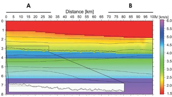
We introduced additional information in the inversion scheme, we assumed that two wells were drilled located at x₌10 km and x₌50 km (Fig. 1). In the last part of the model there is no basalt layer hence the signal coherence is preserved making it pos-sible to identify and pick normal incidence reflections from the basement. Inverting this

10

phase, a reliable estimation of the top of the basement was obtained for the last 25 km of the model which, jointly with the velocity obtained in first arrival inversions, con-strained the model in this part. This results were extrapolated under the basalt layer and used as starting model to invert reflections and refractions from the basement which yielded to our final model where the theoretical model is reasonably well

recov-15

ered (Fig. 8). Note that additional information is required by the travel time inversion methods to obtain reliable models.

5 Metropolis simulations

Statistical methods maybe used in order to assess the reliability of inverted velocity models. Among them, probably Monte-Carlo based simulations are the most used.

20

These consist of generating a relatively large number of random velocity models from the same starting model and performing an inversion for each starting model. Finally, the results ara compared to asses which model fits the data the best. This method is also used to test the reliability of the starting model in a inversion scheme and the stability of the results (Korenaga et al., 2000; Sallar `es et al., 2003; Mart´ıet al., 2006).

25

(10)

SED

5, 189–226, 2013

I. Flecha et al.

Title Page

Tables Figures

◭ ◮

Back Close

Full Screen / Esc

Discussion

P

a

per

|

Dis

cussion

P

a

per

|

Discussion

P

a

per

|

Discussio

n

P

a

per

Metropolis algorithms (Metropolis et al., 1953) take advantage of the a priori knowl-edge of the previous model in the iterative scheme. In the first stages of the simulation the influence of the starting model is clear but, after some iterations, this influence decreases considerably, this is known as “burn-in”. Using this technique the whole re-gion of allowed paremeters is visited which yields a random walk within the rere-gion of

5

possible parameters. A scheme of the algorithm is shown in Fig. 9 and a detailed de-scription of the methodology can be found in Pearse (2002). In this case, Rayinvr (Zelt and Smith, 1992) was used to solve the forward problem and to calculate χ2 which provides the likelihood for every model. The iterative process starts using the starting model (in this case the real model used to build synthetic data) as the current model,

10

then this was randomly modified to generate a new model. Then, the reliability of the model was tested based on the ratio obtained from dividing the likelihood of the current model versus the likelihood of the new model:

– If the ratio was equal or larger than one, the new model was accepted and the new model became the current model.

15

– If ratio was smaller than one, a random number between 1 and 0 was calculated and another test was performed:

– If the ratio was larger than the random number, the new model was accepted and the new model became the current model.

– If the ratio was smaller than the random number, the new model was rejected

20

and the current model remained unchanged.

The process is repeated for a large number of iterations giving as a result a set of different models that reasonably fit the picked travel times when a picking uncertainty is given. In this study, 40 000 iterations were performed for every case in order to obtain a set large enough to have a statistical value. The allowed variations in velocity, thickness

25

(11)

SED

5, 189–226, 2013

I. Flecha et al.

Title Page

Tables Figures

◭ ◮

Back Close

Full Screen / Esc

Discussion

P

a

per

|

Dis

cussion

P

a

per

|

Discussion

P

a

per

|

Discussio

n

P

a

per

|

for subbasalt layer and 10% for basement (Table 3). Variations were chosen increasing in depth to account for the lost of accuracy in deeper layers.

Some synthetic shots have been generated using different 1-D models and two dif-ferent frequencies 10 Hz and 20 Hz (Figs. 10 and 11):

– Model 1: model with subbasalt low velocity layer.

5

– Model 2: the same as model 1 but with a thicker basalt layer.

5.1 Model 1: results

The first analysis was done on the data from model 1 and 10 Hz. In this case, refraction from basalt layer seems to be very clear as shown in Fig. 10. However, this yields a phase identification which is not correct because the phase identified as a refraction

10

from basalt layer is the interference between two phases: refraction from basalt and reflection from the base of the basalt. To emphasize this effect, a shotgather was cal-culated using model 1 but replacing the subbasalt velocity by a layer of 5 km s−1_{, in}

this way no reflection in the base of the basalt layer was generated obtaining a pure refraction in the basalt layer. This pure refraction was picked and compared with the

15

identified in the previous case (Fig. 12). Thus, in the first case, we have identified an interference between basalt refraction and base basalt reflection as a pure refraction which is erroneous.

Using the picks from the data obtained with model 1 in the Metropolis approach with a high picking error (see Table 4) and considering 40 000 different cases, we obtained

20

an overestimation in both, velocity and thickness of the subbasalt layer (Fig. 13). By reducing the picking error (case with low uncertainty) we would expect a better corre-lation between the more probable model and the theoretical one. In practice, under the same conditions but reducing the picking uncertaity, a worse result was obtained where there was no need of a subbasalt low velocity layer in order to fit the data (Fig. 14). This

25

(12)

SED

5, 189–226, 2013

I. Flecha et al.

Title Page

Tables Figures

◭ ◮

Back Close

Full Screen / Esc

Discussion

P

a

per

|

Dis

cussion

P

a

per

|

Discussion

P

a

per

|

Discussio

n

P

a

per

basalt. Therefore what was labelled as basalt refraction is within the allowed range of times for this phase. On the other hand, by reducing the picking error, the range of times do not include the real refraction and then our erroneous phase identification yields the unexpected result of Fig. 14.

The same analysis was repeated using model 1 and data generated with 20 Hz. In

5

this case results are better and fit the right model (Fig. 15).

5.2 Model 2: results

In model 2 the thickness of basalt layer was increased to test if it was possible to use a well identified base basalt reflection to constrain better the thickness and velocity of this layer. Two different simulations have been performed: one using a very

conserva-10

tive picking and avoiding picks in the “interference zone” (basalt refraction/base basalt reflection) displayed in Fig. 12 and another including more picks. For the first case (Fig. 16) the velocity gradient for basalt layer was well reproduced while for the second case (Fig. 17) this gradient did not fit the real model. For the basement velocity gradient the result was the opposite, obtaining a better result when considering a larger number

15

of picks. In both cases, subbasalt velocity layer is not reliably recovered. As in model 1, better fit is obtained for 20 Hz data (Fig. 18), where the velocity gradient for basalt and basement are well reproduced. Again, in both cases, the subbasalt layer is not well recovered.

The Metropolis study reveals that the phase identification is a critical step. Despite

20

objectivity provided by mathematics used in the inversion, phase identification turns travel time tomography in a subjective procedure. Additionally, uncertainty is also a crit-ical parameter in the inversion which can influence the inversion algorithm. Moreover, considering data with different frequency content also has an effect on the selection of the most probable model. Not all models required a low velocity layer and there was an

25

(13)

SED

5, 189–226, 2013

I. Flecha et al.

Title Page

Tables Figures

◭ ◮

Back Close

Full Screen / Esc

Discussion

P

a

per

|

Dis

cussion

P

a

per

|

Discussion

P

a

per

|

Discussio

n

P

a

per

|

Synthetic shots were created using a full-waveform code while likelihood was cal-culated using a ray tracing code. Full-waveform techniques are more accurate than ray tracing methods because they take into account information about the amplitudes, which are ignored in ray tracing simulations. Due to the high computational cost of full-waveform methodologies, ray tracing methods are still conventionally used to

ob-5

tain velocity models (Pratt et al., 1996). These results suggest that conventional travel time inversion (tomography) schemes without additional information are not sufficient to constrain the base of basalt or subbasalt geological structures.

In the synthetic tests performed in this study no noise has been considered. In this sense, some features that commonly are present in real data as tidal noise,

electri-10

cal noise and some other e_ffects a_ffecting the quality of the data, have not been in-cluded. Results derived from these tests must be interpreted as results obtained in ideal conditions and in consequence, the best ones expected for a real case using this methodology.

6 Conclusions

15

This study, which involves synthetic data suggests that there are some physical limita-tions to obtain a reliable velocity model for subbasalt zones in areas covered by high velocity rocks (like basalts and salts). In the case of thin basalt layers, the base basalt reflection is totally masked within the water-wave cone and it cannot be separated from the basalt refraction. There are several subjective factors that can affect and condition

20

the results from the inversion as maximum picking offset or picking uncertainty. An-other important point is the frequency content of the signal, our Metropolis simulations suggest that the original model is best recovered using high frequencies and thicker basalt. This result is relevant because the actual tendency is using and designing air-guns that produce low frequency data as single bubble source. The most critical point

25

(14)

SED

5, 189–226, 2013

I. Flecha et al.

Title Page

Tables Figures

◭ ◮

Back Close

Full Screen / Esc

Discussion

P

a

per

|

Dis

cussion

P

a

per

|

Discussion

P

a

per

|

Discussio

n

P

a

per

basalt (refraction) and, the base basalt reflection is a key element in determining the correct thickness of the basalt. The uncertainty associated to the travel time picks is also a relevant issue, as it can not distinguish between high and low velocity subbasalt structures. Moreover, a wrong determination of the basalt thickness and velocity has a direct influence on the resulting model for layers under the basalt. Reliable subbasalt

5

imaging with wide-angle reflection/refraction datasets requires additional information as the knowledge on the thickness of the basalt at some point and its internal veloc-ity distribution. This could be achieved by using other methodologies to infere basalt properties.

Acknowledgements. Funding for this research was provided by SINDRI (Quantitative

evalua-10

tion of the existing technologies for imaging within basalt-covered areas from the Faroes re-gion), the Spanish Ministry of Science and Technology (Ref: CGL2004-04623/BTE) and Gen-eralitat de Catalunya (Ref: 2005SGR00874). We are grateful to Immo Trinks for training in the use of the TTT code.

References

15

Carmichael, R. S.: Handbook of Physical Properties of rocks, vol. II, CSC Press, Boston, 1982. 193, 205

Christensen, N. I. and Mooney, W. D.: Seismic velocity structure and composition of the conti-nental crust: A global view, J. Geophys. Res., 100, 9761–9788, 1995. 205

Flecha, I., Mart´_ı, D., Carbonell, R., Escuder-Viruete, J., and P ´erez-Esta ´un, A.: Imaging low

20

velocity anomalies with the aid of seismic tomography, Tectonophysics, 388, 225–238, 2004. 190

Fliedner, M. M. and White, R. S.: Depth imaging of basalt flows in the Faeroe-Shetland Basin, Geophys. J. Int., 152, 353–371, 2003. 192

Goff, J. A. and Jordan, T. H.: Stochastic modeling of seafloor morphology: inversion of sea

25

beam data for second-order statistics, J. Geophys. Res., 96, 13589–13608, 1988. 193 Hughes, S., Barton, P. J., and Harrison, D.: Exploration in the Shetland-Faeroe Basin using

(15)

SED

5, 189–226, 2013

I. Flecha et al.

Title Page

Tables Figures

◭ ◮

Back Close

Full Screen / Esc

Discussion

P

a

per

|

Dis

cussion

P

a

per

|

Discussion

P

a

per

|

Discussio

n

P

a

per

|

Jegen-Kulcsar, M. and Hobbs, R. W.: Outline of a joint inversion of gravity, MT and seismic data, Annales Societatis Scientiarum Færoensis, 43, 163–167, 2005. 193

Korenaga, J., Holbrook, W. S., Kent, G. M., Kelemen, P. B., Detrick, R. S., Larsen, H. C., Hopper, J. R., and Dahl-Jensen, T.: Crustal structure of the Southeast Greeenland margin from joint refraction and reflection seismic tomography, J. Geophys. Res., 105, 21591–21614, 2000.

5

197

Martini, F. and Bean, C. J.: Interface scattering versus body scattering in subbasalt imaging and application of prestack wave equation datuming, Geophysics, 67, 1593–1601, 2002. 193 Martini, F., Bean, C. J., Dolan, S., and Marsan, D.: Seismic image quality beneath strongly

scat-tering structures and implications for lower crustal imaging: numerical simulations, Geophys.

10

J. Int., 145, 423–435, 2001. 193

Mart´ı, D., Carbonell, R., Escuder-Viruete, J., and P ´erez-Esta ´un, A.: Characterization of a frac-tured granitic pluton: P- and s-waves seismic tomography and uncertainty analysis, Tectono-physics, 422, 99–114, 2006. 197

Metropolis, N., Rosenbluth, A. W., Rosenbluth, M. N., and Teller, A. H.: Equation of state

calcu-15

lations by fast computing machines, J. Chem. Phys., 21, 1087–1092, 1953. 198

Pearse, S.: Inversion and modelling of seismic data to assess the evolution of the Rockall Trough, Ph.D. thesis, Cambridge University, 2002. 198, 217

Pratt, R. G., Song, Z. M., Williamson, P., and Warner, M.: Two-dimensional velocity models from wide-angle seismic data by wavefield inversion, Geophys. J. Int., 124, 323–340, 1996. 201

20

Raum, T., Mjelde, R., Berge, A. M., Paulsen, J. T., Digranes, P., Shimamura, H., Shiobara, H., Kodaira, S., Larsen, V. B., Fredsted, R., Harrison, D. J., and Johnson, M.: Sub-basalt struc-tures east of the Faroe Islands revealed from wide-angle seismic and gravity data, Petrol. Geosci., 11, 291–308, 2005. 192

Richardson, K. R., Smallwood, J. R., White, R. S., Snyder, D. B., and Maguire, P. K. H.: Crustal

25

structure beneath the Faroe Islands and the Faroe-Iceland Ridge, Tectonophysics, 300, 159– 180, 1995. 192

Richardson, K. R., White, R. S., England, R. W., and Fruehn, J.: Crustal structure east of the Faroe Islands: mapping sub-basalt sediments using wide-angle seismic data, Petrol. Geosci., 5, 161–172, 1999. 191, 192

30

(16)

SED

5, 189–226, 2013

I. Flecha et al.

Title Page

Tables Figures

◭ ◮

Back Close

Full Screen / Esc

Discussion

P

a

per

|

Dis

cussion

P

a

per

|

Discussion

P

a

per

|

Discussio

n

P

a

per

Sallar `es, V., Charvis, P., Flueh, E. R., and Bialas, J.: Seismic structure of Cocos and Malpelo Ridges and implications for hot spot-ridge interaction, J. Geophys. Res., 108, 2564, doi:10.1029/2003JB002431, 2003. 197

Sava, P. and Biondi, B.: Wave-equation migration velocity analysis. II. Subsalt imaging exam-ples, Geophys. Prosp., 52, 607–623, 2004. 190

5

Smallwood, J. R., Towns, M. J., and White, R. S.: The structure of the Faeroe-Shetland Trough from integrated deep seismic and potential field modelling, J. Geol. Soc., 158, 409–412, 2001. 192

Sochacki, J. S., Kubichek, R., George, J. H., Fletcher, W. R., and Smithson, S. B.: Absorbing boundary conditions and surface waves, Geophysics, 52, 60–71, 1987. 193

10

Sochacki, J. S., George, J. H., Ewing, R. E., and Smithson, S. B.: Interface conditions for acous-tic and elasacous-tic wave propagation, Geophysics, 56, 168–181, 1991. 193

Sørensen, A. B.: Cenozoic basin development and stratigraphy of the Faroes area, Petrol. Geosci., 9, 189–207, 2003. 192

Staples, R. K., Hobbs, R. W., and White, R. S.: A comparison between airguns and explosives

15

as wide-angle seismic sources, Geophys. Prosp., 47, 313–339, 1999. 192

Trinks, I.: Traveltime tomography of densely sampled seismic data, Ph.D. thesis, Cambridge University, 2003. 194

Trinks, I., Singh, S. C., Chapman, C. H., Barton, P. J., Bosch, M., and Cherrett, A.: Adaptative traveltime tomography of densely sampled seismic data, Geophys. J. Int., 160, 925–938,

20

2005. 194, 211, 212

White, R. S., Christie, P. A. F., Kusznir, N. J., Roberts, A., Davies, A., Hurst, N., Lunnon, Z., Parkin, C. J., Roberts, A. W., Smith, L. K., Spitzer, R., Surendra, A., and Tymms, V.: iSIMM pushes frontiers of marine seismic acquisition, First Break, 20, 782–786, 2002. 193

White, R. S., Smallwood, J. R., Fliedner, M. M., Boslaugh, B., Maresh, J., and Fruehn, J.:

Imag-25

ing and regional distribution of basalt flows in the Faroe-Shetland Basin, Geophys. Prosp., 51, 215–231, 2003. 191, 192

Williamson, P.: Introduction, Geophys. Prosp., 53, 167–168, 2003. 190

Zelt, C. A. and Smith, R. B.: Seismic traveltime inversion for 2-D crustal velocity structure, Geophys. J. Int., 108, 16–34, 1992. 191, 198

30

(17)

SED

5, 189–226, 2013

I. Flecha et al.

Title Page

Tables Figures

◭ ◮

Back Close

Full Screen / Esc

Discussion

P

a

per

|

Dis

cussion

P

a

per

|

Discussion

P

a

per

|

Discussio

n

P

a

per

|

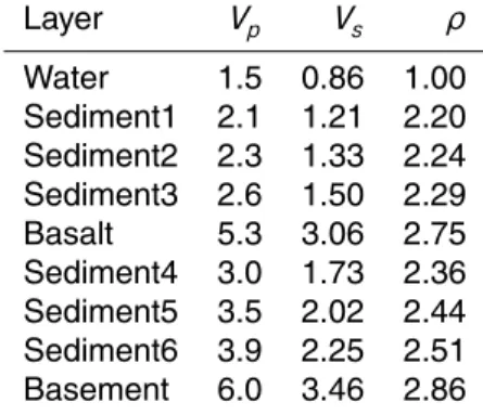
Table 1.Velocities and densities used in the synthetic model. Physical properties were taken from Carmichael (1982). The Poisson ratio was 0.25 and the density was calculated using the Christensen relation Christensen and Mooney, (1995):ρ=1.85+0.169V_p.

Layer V_p V_s ρ

(18)

SED

5, 189–226, 2013

I. Flecha et al.

Title Page

Tables Figures

◭ ◮

Back Close

Full Screen / Esc

Discussion

P

a

per

|

Dis

cussion

P

a

per

|

Discussion

P

a

per

|

Discussio

n

P

a

per

Table 2.Parameters used to generate synthetic data.

Synthetic data parameters

Model length 100 km

Model depth 8 km

Cell size 10×10 m

Number of shots 80

Number of channels 3294

Station spacing 30 m

Recording length 30 s

Source spacing 1 km

(19)

SED

5, 189–226, 2013

I. Flecha et al.

Title Page

Tables Figures

◭ ◮

Back Close

Full Screen / Esc

Discussion

P

a

per

|

Dis

cussion

P

a

per

|

Discussion

P

a

per

|

Discussio

n

P

a

per

|

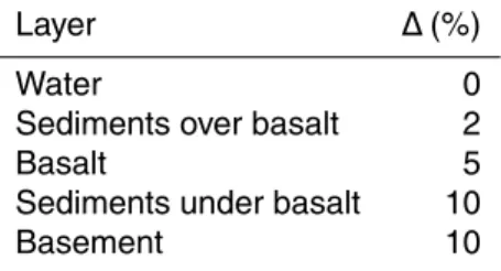
Table 3.Allowed variation to generate modified models for velocity, velocity gradient and thick-ness for every layer in models 1 and 2.

Layer ∆(%)

Water 0

Sediments over basalt 2

Basalt 5

Sediments under basalt 10

(20)

SED

5, 189–226, 2013

I. Flecha et al.

Title Page

Tables Figures

◭ ◮

Back Close

Full Screen / Esc

Discussion

P

a

per

|

Dis

cussion

P

a

per

|

Discussion

P

a

per

|

Discussio

n

P

a

per

Table 4.Picking uncertainty in ms for every layer considered in metropolis algorithm.

Phase model1 model1 model2 model2

10 Hz 20 Hz 10 Hz 20 Hz

Seabed reflection 8 8 8 8 8

Top basalt reflection 24 16 16 24 16

Basalt refraction 50 24 24 50 24

Top basement reflection 100 50 50 100 50

Basement refraction 100 50 50 100 50

(21)

SED

5, 189–226, 2013

I. Flecha et al.

Title Page

Tables Figures

◭ ◮

Back Close

Full Screen / Esc

Discussion

P

a

per

|

Dis

cussion

P

a

per

|

Discussion

P

a

per

|

Discussio

n

P

a

per

|

(22)

SED

5, 189–226, 2013

I. Flecha et al.

Title Page

Tables Figures

◭ ◮

Back Close

Full Screen / Esc

Discussion

P

a

per

|

Dis

cussion

P

a

per

|

Discussion

P

a

per

|

Discussio

n

P

a

per

(23)

SED

5, 189–226, 2013

I. Flecha et al.

Title Page

Tables Figures

◭ ◮

Back Close

Full Screen / Esc

Discussion

P

a

per

|

Dis

cussion

P

a

per

|

Discussion

P

a

per

|

Discussio

n

P

a

per

|

(24)

SED

5, 189–226, 2013

I. Flecha et al.

Title Page

Tables Figures

◭ ◮

Back Close

Full Screen / Esc

Discussion

P

a

per

|

Dis

cussion

P

a

per

|

Discussion

P

a

per

|

Discussio

n

P

a

per

(25)

SED

5, 189–226, 2013

I. Flecha et al.

Title Page

Tables Figures

◭ ◮

Back Close

Full Screen / Esc

Discussion

P

a

per

|

Dis

cussion

P

a

per

|

Discussion

P

a

per

|

Discussio

n

P

a

per

|

(26)

SED

5, 189–226, 2013

I. Flecha et al.

Title Page

Tables Figures

◭ ◮

Back Close

Full Screen / Esc

Discussion

P

a

per

|

Dis

cussion

P

a

per

|

Discussion

P

a

per

|

Discussio

n

P

a

per

(27)

SED

5, 189–226, 2013

I. Flecha et al.

Title Page

Tables Figures

◭ ◮

Back Close

Full Screen / Esc

Discussion

P

a

per

|

Dis

cussion

P

a

per

|

Discussion

P

a

per

|

Discussio

n

P

a

per

|

(28)

SED

5, 189–226, 2013

I. Flecha et al.

Title Page

Tables Figures

◭ ◮

Back Close

Full Screen / Esc

Discussion

P

a

per

|

Dis

cussion

P

a

per

|

Discussion

P

a

per

|

Discussio

n

P

a

per

(29)

SED

5, 189–226, 2013

I. Flecha et al.

Title Page

Tables Figures

◭ ◮

Back Close

Full Screen / Esc

Discussion

P

a

per

|

Dis

cussion

P

a

per

|

Discussion

P

a

per

|

Discussio

n

P

a

per

|

(30)

SED

5, 189–226, 2013

I. Flecha et al.

Title Page

Tables Figures

◭ ◮

Back Close

Full Screen / Esc

Discussion

P

a

per

|

Dis

cussion

P

a

per

|

Discussion

P

a

per

|

Discussio

n

P

a

per

(31)

SED

5, 189–226, 2013

I. Flecha et al.

Title Page

Tables Figures

◭ ◮

Back Close

Full Screen / Esc

Discussion

P

a

per

|

Dis

cussion

P

a

per

|

Discussion

P

a

per

|

Discussio

n

P

a

per

|

(32)

SED

5, 189–226, 2013

I. Flecha et al.

Title Page

Tables Figures

◭ ◮

Back Close

Full Screen / Esc

Discussion

P

a

per

|

Dis

cussion

P

a

per

|

Discussion

P

a

per

|

Discussio

n

P

a

per

(33)

SED

5, 189–226, 2013

I. Flecha et al.

Title Page

Tables Figures

◭ ◮

Back Close

Full Screen / Esc

Discussion

P

a

per

|

Dis

cussion

P

a

per

|

Discussion

P

a

per

|

Discussio

n

P

a

per

|

(34)

SED

5, 189–226, 2013

I. Flecha et al.

Title Page

Tables Figures

◭ ◮

Back Close

Full Screen / Esc

Discussion

P

a

per

|

Dis

cussion

P

a

per

|

Discussion

P

a

per

|

Discussio

n

P

a

per

(35)

SED

5, 189–226, 2013

I. Flecha et al.

Title Page

Tables Figures

◭ ◮

Back Close

Full Screen / Esc

Discussion

P

a

per

|

Dis

cussion

P

a

per

|

Discussion

P

a

per

|

Discussio

n

P

a

per

|

(36)

SED

5, 189–226, 2013

I. Flecha et al.

Title Page

Tables Figures

◭ ◮

Back Close

Full Screen / Esc

Discussion

P

a

per

|

Dis

cussion

P

a

per

|

Discussion

P

a

per

|

Discussio

n

P

a

per

(37)

SED

5, 189–226, 2013

I. Flecha et al.

Title Page

Tables Figures

◭ ◮

Back Close

Full Screen / Esc

Discussion

P

a

per

|

Dis

cussion

P

a

per

|

Discussion

P

a

per

|

Discussio

n

P

a

per

|

(38)

SED

5, 189–226, 2013

I. Flecha et al.

Title Page

Tables Figures

◭ ◮

Back Close

Full Screen / Esc

Discussion

P

a

per

|

Dis

cussion

P

a

per

|

Discussion

P

a

per

|

Discussio

n

P

a

per