On the optimal method for evaluating cloud products from passive satellite imagery using CALIPSO-CALIOP data: example investigating the CM SAF CLARA-A1 dataset

(1)

AMTD

6, 1093–1141, 2013

Investigating the CM SAF CLARA-A1

dataset

K.-G. Karlsson and E. Johansson

Title Page

Abstract Introduction

Conclusions References

Tables Figures

◭ ◮

Back Close

Full Screen / Esc

Printer-friendly Version Interactive Discussion

Discussion

P

a

per

|

Dis

cussion

P

a

per

|

Discussion

P

a

per

|

Discussio

n

P

a

per

|

Atmos. Meas. Tech. Discuss., 6, 1093–1141, 2013 www.atmos-meas-tech-discuss.net/6/1093/2013/ doi:10.5194/amtd-6-1093-2013

Atmospheric Measurement

Techniques

Open Access

Discussions

Geoscientiic Geoscientiic

This discussion paper is/has been under review for the journal Atmospheric Measurement Techniques (AMT). Please refer to the corresponding final paper in AMT if available.

On the optimal method for evaluating

cloud products from passive satellite

imagery using CALIPSO-CALIOP data:

example investigating the CM SAF

CLARA-A1 dataset

K.-G. Karlsson and E. Johansson

Swedish Meteorological and Hydrological Institute, Norrk ¨oping, Sweden

Received: 9 January 2013 – Accepted: 23 January 2013 – Published: 1 February 2013

Correspondence to: K.-G. Karlsson (karl-goran.karlsson@smhi.se) and E. Johansson (erik.johansson@smhi.se)

Published by Copernicus Publications on behalf of the European Geosciences Union.

(2)

AMTD

6, 1093–1141, 2013

dataset

Title Page

Tables Figures

◭ ◮

Back Close

Full Screen / Esc

Discussion

P

a

per

|

Dis

cussion

P

a

per

|

Discussion

P

a

per

|

Discussio

n

P

a

per

|

Abstract

A method for detailed evaluation of a new satellite-derived global 28-yr cloud and radi-ation climatology (Climate Monitoring SAF Cloud, Albedo and Radiradi-ation dataset from AVHRR data, named CLARA-A1) from polar orbiting NOAA and Metop satellites is presented. The method combines 1 km and 5 km resolution cloud datasets from the

5

CALIPSO-CALIOP cloud lidar for estimating cloud detection limitations and the accu-racy of cloud top height estimations.

Cloud detection is shown to work e_fficiently for clouds with optical thicknesses above 0.30 except for at twilight conditions when this value increases to 0.45. Some misclas-sifications generating erroneous clouds over land surfaces in semi-arid regions in the

10

sub-tropical and tropical regions are revealed. In addition, a substantial fraction of all clouds remains undetected in the Polar regions during the polar winter season due to the lack of or an inverted temperature contrast between Earth surfaces and clouds.

Subsequent cloud top height evaluation took into account the derived information about the cloud detection limits. It was shown that this has fundamental importance

15

for the achieved results. An overall bias of−274 m was achieved compared to a bias

of−2762 m if no measures were taken to compensate for cloud detection limitations.

Despite this improvement it was concluded that high-level clouds still su_ffer from sub-stantial height underestimations while the opposite is true for low-level (boundary layer) clouds.

20

(3)

AMTD

6, 1093–1141, 2013

dataset

Title Page

Tables Figures

◭ ◮

Back Close

Full Screen / Esc

Discussion

P

a

per

|

Dis

cussion

P

a

per

|

Discussion

P

a

per

|

Discussio

n

P

a

per

|

1 Introduction

The introduction of the A-Train (i.e. Aqua Train or sometimes referred to as the After-noon Train) series of satellites (Stephens et al., 2002) has been a major milestone for cloud research and for satellite meteorology in general. For the first time in history, a series of satellites and sensors are able to provide not only the global coverage of

5

cloud fields and aerosols but also the vertical structure of clouds and aerosols and their respective properties. The vertical probing capability was in particular associated with the launch of the CloudSat (Stephens et al., 2002) and CALIPSO (Winker et al., 2009) missions in 2006 since both satellites are carrying active sensors – a cloud profiling radar (CPR) on CloudSat and a cloud and aerosol lidar (CALIOP) on CALIPSO. These

10

satellites have now produced more than five years of data. It means that despite the relatively limited spatial sampling capability from the polar orbit (i.e. a consequence of both active sensors operating exclusively in nadir view) the long time series now offers enough measurements to become useful also for studying mean conditions (approach-ing the estimation of climatologies) in parallel to the more obvious use in case-to-case

15

process-oriented studies. Good examples of this and of methods and tools aiming at climatological studies are given by Stubenrauch et al. (2012), Cesana et al. (2012), Liu et al. (2012), Devasthale and Thomas (2011), Chepfer et al. (2010), and Delano ¨e et al. (2011). In addition, the improved statistical significance of the datasets now make them very useful as “ground truth” datasets for training of cloud algorithms (Heidinger

20

et al., 2012). Similarly, an important application is the use for more thorough evalua-tion of cloud products from various algorithms based on data from other satellite plat-forms. This concerns especially those based on data from wider-swath scanning sen-sors measuring in visible, infrared, and microwave spectral regions (i.e. data from pas-sive imagers) as being demonstrated by Holz et al. (2008), Minnis et al. (2008), Reuter

25

et al. (2009), Heidinger and Pavolonis (2009), and Karlsson and Dybbroe (2010). The information from the CALIPSO-CALIOP lidar is particularly interesting since this sensor is undoubtedly much more sensitive to the presence of clouds in the

(4)

AMTD

6, 1093–1141, 2013

dataset

Title Page

Tables Figures

◭ ◮

Back Close

Full Screen / Esc

Discussion

P

a

per

|

Dis

cussion

P

a

per

|

Discussion

P

a

per

|

Discussio

n

P

a

per

|

atmosphere than any other space-born sensor at hand. Because of this it has the potential of being used for establishing a firm knowledge of the cloud detection limit for other cloud retrieval methods based on data from other satellite sensors. This as-pect is of fundamental importance for securing an optimal and unambiguous use of the information from various cloud retrieval algorithms. An important application in this

5

respect is the method for how to compare satellite-derived cloud parameters to infor-mation simulated by climate models and numerical weather prediction (NWP) models. To ensure an appropriate inter-comparison here specific tools have been developed. The most well-established tool is the Cloud Feedback Model Inter-comparison Project (CFMIP) Observational Simulation Package (COSP) which is described by

Bodas-10

Salcedo et al. (2011). For all the cloud datasets being simulated by COSP from model data, the information on which clouds are detected or not by the various satellite sen-sors is essential for assuring an appropriate inter-comparison of model and observation datasets.

This paper focuses on the use of CALIPSO-CALIOP data for evaluating the cloud

de-15

tection limitations of the methods used to derive one particular satellite-derived climate data record; the CLARA-A1 dataset. The acronym stands for the Climate Monitoring Satellite Application Facility (CM SAF – see www.cmsaf.eu and Schulz et al., 2009) Cloud, Albedo, and Radiation dataset from AVHRR data (Karlsson et al., 2013). It is based on global historic Advanced Very High Resolution Radiometer (AVHRR) data

20

from the polar orbiting NOAA satellites covering the period 1982 until 2009.

While working with the evaluation, several issues related to how to interpret the CALIPSO-CALIOP cloud datasets aroused. This was mainly triggered by the notifi-cation of some inconsistencies between CALIOP cloud datasets created at di_fferent spatial resolutions. We claim that these differences have so far not been accounted for

25

(5)

AMTD

6, 1093–1141, 2013

dataset

Title Page

Tables Figures

◭ ◮

Back Close

Full Screen / Esc

Discussion

P

a

per

|

Dis

cussion

P

a

per

|

Discussion

P

a

per

|

Discussio

n

P

a

per

|

Section 2 introduces the two datasets to be inter-compared and Sect. 3 elaborates further on the problems associated with this comparison and suggests a method on how to deal with them. This is followed in Sect. 4 by the presentation of results on the performance of cloud detection, its regional dependency and the apparent cloud detection limit in terms of the thinnest (in the cloud optical thickness sense) clouds

5

being detected. Sect. 5 presents results for the cloud top height determination, taking into account the deduced cloud detection limitations. Finally, Sect. 6 concludes and gives some further discussion on the optimal method to be used for cloud parameter validation.

2 Data 10

2.1 The investigated dataset: CLARA-A1

The CLARA-A1 dataset of global cloud products retrieved by CM SAF cloud retrieval methods is based on reduced resolution (approximately 4 km) global area coverage (GAC) AVHRR data spanning the time period 1982–2009. The total set of cloud prod-ucts includes Cloud Fractional Cover, Cloud Top Level, Cloud Optical Thickness, Cloud

15

Phase, Liquid Water Path, Ice Water Path, and Joint Cloud property histograms. Here, we will concentrate on the evaluation of the first two products. For a full description of the dataset the reader is referred to Karlsson et al. (2013).

The Cloud Fractional Cover (CFC) product is derived directly from results of a cloud screening or cloud masking method. CFC is defined as the fraction of cloudy pixels per

20

grid square compared to the total number of analysed pixels in the grid square. Frac-tional cloud cover is expressed in percent. The product is calculated using the Now-casting Satellite Application Facility (NWC SAF) PPS (Polar Platform System) cloud mask algorithm (see http://www.nwcsaf.org/ for details on the NWC-SAF project). The algorithm (detailed by Dybbroe et al., 2005) is based on a multi-spectral thresholding

25

technique applied to every pixel of the satellite scene. Several threshold tests may be

(6)

AMTD

6, 1093–1141, 2013

dataset

Title Page

Tables Figures

◭ ◮

Back Close

Full Screen / Esc

Discussion

P

a

per

|

Dis

cussion

P

a

per

|

Discussion

P

a

per

|

Discussio

n

P

a

per

|

applied (and must be passed) before a pixel is assigned to be cloudy or cloud-free. Thresholds are determined from present viewing and illumination conditions and from the current atmospheric state (prescribed by data assimilation products from numerical weather prediction models – here, the ERA-Interim dataset, see Dee et al. (2011) and http://www.ecmwf.int/research/era/do/get/era-interim). Also ancillary information about

5

surface status (e.g. land use categories and surface emissivities) is taken into account. Thus, thresholds are dynamically defined and therefore unique for each individual pixel. The Cloud Top Level (CTO) product is also derived using NWC SAF PPS algorithms. The product is abbreviated CTO because it can be expressed in three alternative forms: cloud top height (in meters), cloud top pressure (in hPa), and cloud top temperature (in

10

Kelvin). In this paper we concentrate on the cloud top height version since this is what is available from the CALIPSO-CALIOP cloud products. Consequently, we will refer to the product as either CTO or cloud top height.

Cloud top processing is sub-divided using two separate algorithms, one for opaque and one for fractional and semi-transparent clouds, and it is applied to all cloudy

pix-15

els as identified by the PPS cloud mask product. The opaque algorithm uses simu-lated cloud free and cloudy top of atmosphere (TOA) 11 µm radiances which are com-pared and matched to measured radiances. Cloudy radiances are simulated assuming “black-body”-clouds at various levels. The semi-transparent algorithm is applied to all pixels classified as semi-transparent cirrus or fractional water cloud. This

classifica-20

tion is based on the analysis of brightness temperature di_fferences of the 11 µm and 12 µm (split window) channels noting that this difference is generally small or negli-gible for opaque clouds. Also brightness temperatures at 3.7 µm are involved in this process. A histogram technique is applied based on the construction of two dimen-sional histograms using AVHRR channel 4 and 5 brightness temperatures composed

25

(7)

AMTD

6, 1093–1141, 2013

dataset

Title Page

Tables Figures

◭ ◮

Back Close

Full Screen / Esc

Discussion

P

a

per

|

Dis

cussion

P

a

per

|

Discussion

P

a

per

|

Discussio

n

P

a

per

|

Obviously, only a small fraction of the CLARA-A1 dataset may be evaluated using CALIPSO-CALIOP data (limited to years 2006–2009). However, it is believed that re-sults should largely be valid also for rere-sults before these years provided that a rea-sonably large number of collocations can be found and if considering that the AVHRR instrument has not undergone drastic changes throughout the years. The basis for the

5

comparison is the use of original PPS cloud mask and cloud top height products for full orbit swaths (about 13 000 scan lines) which are collocated with CALIPSO-CALIOP orbits using specific matching criteria (further described in Sect. 3).

In the remainder of the text we will use the notation CLARA-A1/PPS to emphasize that we examine the performance of the PPS cloud mask and PPS cloud top height

10

products for the PPS version used when defining the CLARA-A1 dataset.

2.2 The reference validation dataset: CALIPSO-CALIOP cloud products

The Cloud-Aerosol Lidar and Infrared Pathfinder Satellite Observation (CALIPSO) satellite was launched in April 2006 together with CloudSat. The satellite carries the Cloud-Aerosol Lidar with Orthogonal Polarization (CALIOP) and the first data became

15

available in August 2006. CALIOP provides detailed profile information about cloud and aerosol particles and corresponding physical parameters. CALIOP measures the backscatter intensity at 1064 nm while two other channels measure the orthogonally polarized components of the backscattered signal at 532 nm. The horizontal resolu-tion of each single field of view (FOV) is 333 m and the vertical resoluresolu-tion is 30–60 m.

20

The CALIOP cloud product we have used reports observed cloud layers, i.e. all lay-ers observed until signal becomes too attenuated. In practice the instrument can only probe the full geometrical depth of a cloud if the total optical thickness is not larger than a certain threshold (somewhere in the range 6–10). For optically thicker clouds only the upper portion of the cloud is sensed.

25

CALIOP products have been retrieved from the NASA Langley Atmospheric Science Data Centre (ASDC, http://eosweb.larc.nasa.gov/JORDER/ceres.html). We have used the Lidar Level 2 Cloud and Aerosol Layer Information product Version 3.01 and the

(8)

AMTD

6, 1093–1141, 2013

dataset

Title Page

Tables Figures

◭ ◮

Back Close

Full Screen / Esc

Discussion

P

a

per

|

Dis

cussion

P

a

per

|

Discussion

P

a

per

|

Discussio

n

P

a

per

|

associated information from the Lidar Level 2 Vertical Feature Mask product. Regard-ing the latter it is important to notice the use here of the categorisation of low-level, medium-level and high-level clouds introduced by the International Satellite Cloud Cli-matology Project (ISCCP). This categorisation uses pressure levels of 680 hPa and 440 hPa to separate the three categories. We will use this classification later for

sep-5

arating results of cloud top height determinations between the three vertical groups of clouds.

The CALIOP products are defined in five di_fferent versions with respect to the along-track resolution ranging from 333 m (individual footprint resolution), 1 km, 5 km, 20 km, and 80 km. The four latter resolutions are consequently constructed from several

origi-10

nal footprints/FOVs. This allows a higher confidence in the correct detection and identi-fication of cloud and aerosol layers compared to when using the original high resolution profiles. For example, the identification of very thin Cirrus clouds is more reliable in the 5 km dataset than in the 1 km dataset since signal-to-noise levels can be raised by using a combined dataset of several original profiles.

15

The natural choice of product resolution for the validation of 4 km AVHRR GAC prod-ucts is to use the CALIOP 5 km dataset. The CALIOP 5 km dataset also offers estima-tion of cloud optical thicknesses of individual layers (not available for finer resoluestima-tion FOVs) which is a very attractive feature since it means that this offers a possibility to analyse cloud detection limits quantitatively.

20

Further details on the CALIPSO-CALIOP cloud retrieval algorithms are given by Vaughan et al. (2004) and Winker et al. (2009).

3 Methodology

3.1 Concern about inconsistencies of CALIOP 1 km and 5 km cloud datasets

One of the central features of CALIOP cloud retrieval algorithms (as outlined by

25

(9)

AMTD

6, 1093–1141, 2013

dataset

Title Page

Tables Figures

◭ ◮

Back Close

Full Screen / Esc

Discussion

P

a

per

|

Dis

cussion

P

a

per

|

Discussion

P

a

per

|

Discussio

n

P

a

per

|

signal-to-noise levels by averaging results from high resolution fields of views into coarse resolution field of views. By doing this it is possible to identify cloud layers that are too thin to be detected in the original fine FOV resolution of 330 m because of high noise levels. This means that in theory the optically thinnest cloud layers will be found in the 80 km FOV resolution CALIOP dataset. Since a lot of concern in climate

5

research for many years has been given to the potential impact of thin and sub-visible Cirrus clouds (Stephens et al., 1990), this capability of the CALIPSO mission has been very much highlighted and numerous reports have been published on this subject (two examples are Haladay and Stephens, 2009; Virts et al., 2010).

However, it is possible that the focus on the thin cloud identification may have led

10

to some drawbacks for the prospect of evaluating the performance of other cloud al-gorithms with a good spatial coverage but a reduced cloud detection capability. To exemplify this problem we can consider the following:

Ideally, if thinner and thinner cloud layers are detected for every step we take in reducing the CALIOP FOV resolution (i.e. 0.3 km→1 km→5 km→20 km→80 km) we 15

should have the following inequality for the retrieved CALIPSO global cloud fraction for the various horizontal FOV resolutions (CFCxkm):

CFC_{0.3 km}<_CFC_{1 km}<_CFC_{5 km}<_CFC_{20 km}<_CFC_{80 km} ₍₁₎

In other words, when reducing resolution we should be able to add thin cloud layers to previously detected cloud layers leading to an overall increase of global cloud fraction.

20

However, in practice Eq. (1) seems not to be fulfilled in all cases. For example, in the collocation dataset which was used here (further detailed in Sect. 3.5) almost 20 % of the cases had higher or equal cloud fractions in the 1 km CALIOP cloud dataset than in the 5 km dataset. Similar experiences have also been reported by scientists working with the evaluation of the MODIS cloud algorithms (R. Kuehn, University of

25

Wisconsin, personal communication, 2012). This raises question marks about to what extent the CALIOP 5 km dataset can really be used for the important task of evaluat-ing cloud detection limits for other cloud retrieval algorithms. Thus, in its present form

(10)

AMTD

6, 1093–1141, 2013

dataset

Title Page

Tables Figures

◭ ◮

Back Close

Full Screen / Esc

Discussion

P

a

per

|

Dis

cussion

P

a

per

|

Discussion

P

a

per

|

Discussio

n

P

a

per

|

this dataset is not ideally suited for this task which has also been expressed by the CALIPSO Science team (D. Winker, personal communication, 2012). What appears to happen is that when aggregating results from several fine resolution FOVs, strong signals from boundary layer clouds have been suppressed (this is done deliberately for increasing sensitivity further) which unfortunately has led to the loss of some cloud

5

layers that existed in the previous fine resolution dataset. Thus, thin layers have been added to coarse resolution datasets but unfortunately some (relatively) thick cloud lay-ers have been lost at the same time. This fact results in unchanged or only relatively modestly increased total cloud fraction and in some cases even slightly reduced total cloud fractions.

10

What complicates things further is that also finer resolution (1 km) CALIOP datasets have been shown to miss some specific cloud layers which cannot be considered as exceptionally thin (as reported by Chan and Comiso, 2011). These cloud layers were reported to be boundary-layer clouds at high latitudes with geometrical thicknesses of less than 1 km and with cloud optical thicknesses lower than 14.

15

Because of these ambiguities in the delineation of global cloudiness we suggest that, while waiting for further upgrades of the CALIOP cloud retrieval algorithms (potentially addressing these limitations), one should try to use the existing information in the 1 km and 5 km CALIOP datasets in a combined way to estimate the true cloud situation as far as possible. In the next sub-section we introduce a method which we believe takes

20

the best from both CALIOP datasets, thereby reducing inherent deficiencies.

3.2 Proposed evaluation of cloud amounts using combined 1 km and 5 km CALIOP datasets

The principle for constructing an optimal cloud dataset from CALIOP 1 km and 5 km datasets is based on the assumption that thick (opaque) clouds are well described by

25

(11)

AMTD

6, 1093–1141, 2013

dataset

Title Page

Tables Figures

◭ ◮

Back Close

Full Screen / Esc

Discussion

P

a

per

|

Dis

cussion

P

a

per

|

Discussion

P

a

per

|

Discussio

n

P

a

per

|

the thinnest clouds (including clouds of the type reported by Chan and Comiso, 2011) are reasonably well depicted in the 5 km dataset as well as thin Cirrus clouds that were not detected at all at 1 km FOV resolution.

Thus, we can construct a new merged cloud dataset by going through the following rather simple post-processing steps:

5

– Step 1: Compute a preliminary cloud fraction (CFC′) at 5 km FOV resolution from the 1 km FOVs.

(Thus, CFC’ can now take the six discrete values of 0 %, 20 %, 40 %, 60 %, 80 % and 100 % for every 5 km FOV).

– Step 2: Set 5 km data to CLOUDY if CFC′>_{50 %.} 10

(If a cloud layer was missing in the 5 km dataset but covering more than 50 % of the involved 1 km FOVs, a new layer will now be added).

– Step 3: If a cloud layer exists at 5 km FOV but NOT at any 1 km FOV

⇒new thin layer detected!

⇒Set 5 km FOV to CLOUDY (or, rather, keep the 5 km dataset unchanged). 15

By these simple steps we believe that we have reduced ambiguities significantly even if steps 2 and 3 still mean that there are undetermined retrieved values of both CFC and cloud optical thickness. For example, in step 2 we might add (or restore) a new 5 km layer but we have no way of giving this new layer a retrieved value of cloud optical thickness (since this quantity is only retrieved for the 5 km FOV dataset and not for the

20

1 km FOV dataset). We have “solved” this by prescribing the new value to optical thick-ness 1.0. This is just to show that we believe that this cloud layer should not belong to the category of very thin cloud layers, thus assuring that it will not be included in subsequent cloud detection limit studies focussing at clouds with low optical thickness values. Furthermore, step 2 means that there could be cases when at 1 km FOV there

25

(12)

AMTD

6, 1093–1141, 2013

dataset

Title Page

Tables Figures

◭ ◮

Back Close

Full Screen / Esc

Discussion

P

a

per

|

Dis

cussion

P

a

per

|

Discussion

P

a

per

|

Discussio

n

P

a

per

|

cloudy 5 km FOV will now be removed which maybe could be questioned. But on the other hand, a 5 km FOV that is less than 50 % cloud-covered should actually in this context not be considered as a fully cloudy FOV. The ambiguity comes from the con-sideration that it could theoretically be a cloud layer that is only partly detected by the 1 km FOVs within the 5 km FOV while in reality it is actually covering the entire 5 km

5

FOV. We simply have not enough information here to judge what the truth is so we have to stay with the simple interpretation resulting from step 2. We actually think this uncertainty is marginal in comparison with the general uncertainty about the true CFC within the 5km FOV. This concerns in particular the entirely “new” thin cloud layers ap-pearing in the 5 km dataset being detected after the averaging procedure for reducing

10

the signal-to-noise levels. These new cloud layers are assumed to cover the entire 5 km FOV but there is actually no way of estimating the true CFC within the 5 km FOV. It is possible that these clouds only cover a fraction of the 5 km FOV. In some sense, it is even possible that these interpreted thin cloud layers might be just broken cloud layers which are optically relatively thick but just covering a small fraction of the 5 km FOV (as

15

suggested by A. Devasthale, personal communication, 2012).

Despite these remaining ambiguities, we believe that the proposed approach yields reasonable results that are more consistent and robust than results based exclusively on either 1 km or 5 km FOVs.

3.3 Method for evaluating cloud detection efficiency and the cloud 20

detection limit

The merged new 5 km CALIOP dataset (compiled according to the method described earlier) now includes information about cloud layers at each 5 km FOV and for each cloud layer an estimated cloud optical thickness is given. Though, important to remem-ber is that for the lowermost layer it might be only a minimum value since the entire

25

(13)

AMTD

6, 1093–1141, 2013

dataset

Title Page

Tables Figures

◭ ◮

Back Close

Full Screen / Esc

Discussion

P

a

per

|

Dis

cussion

P

a

per

|

Discussion

P

a

per

|

Discussio

n

P

a

per

|

a filtering mode where cloudy columns having an integrated cloud optical thickness below a certain value are treated as being cloud-free. In this way we should be able to quantify the cloud detection limit of the CLARA-A1 dataset. For this purpose we have filtered the CALIOP dataset in cloud optical thickness steps of 0.05 in the range 0.0–0.5 and in steps of 0.1 in the range 0.5–1.0.

5

For quantifying results we have use the following statistical scores:

1. Mean-error (Bias)

2. Root Mean Square Error (RMS)

3. Probability of Detection (POD) for both cloudy and cloud-free conditions

4. False Alarm Rate (FAR) for both cloudy and cloud-free conditions

10

5. Hit Rate (HR)

6. Kuiper’s skill score (KSS)

For the estimation of cloud occurrence or cloud fractional cover (CFC), we have used a binary representation of the results (i.e. cloud cover₌1 for cloudy conditions and cloud cover=0 for cloud-free conditions) for each individual pixel or FOV.

Conse-15

quently, results are accumulated over the full matchup track to get a mean CFC (ac-cording to Eq. 2 below) and the associated Bias and RMS values. As a final step, all matchup results for all matched orbits are accumulated and averaged.

CFC=

P cloudy P

allpixels (2)

For the remaining four quantities we have used the following definitions (referring to

20

notations in the contingency matrix in Table 1):

POD_cloudy₌ d

c₊d (3)

(14)

AMTD

6, 1093–1141, 2013

dataset

Title Page

Tables Figures

◭ ◮

Back Close

Full Screen / Esc

Discussion

P

a

per

|

Dis

cussion

P

a

per

|

Discussion

P

a

per

|

Discussio

n

P

a

per

|

POD_cloud-free=_aa

+b (4)

FAR_cloudy₌ b

b₊d (5)

FAR_cloud-free₌ c

a₊c (6)

HR₌ a+d

a₊b₊c₊d where 0≤HR≤1 (7)

KSS₌ a·d−c·b

(a₊b₎·(c₊d₎ where −1≤KSS≤1 (8)

5

The POD and FAR quantities estimate how e_fficient CLARA-A1/PPS is in determin-ing either cloudy or cloud-free conditions. Naturally, we want POD values to be as high as possible and FAR values to be minimized. The hit rate HR is a condensed measure

10

of the overall e_fficiency of cloud detection. Finally, the KSS quantity is a complementing measure since the HR can sometimes be misleading because it is heavily influenced by the results for the most common category. For example, if a case is almost totally cloud free but all the few cloudy portions are misclassified as cloud-free by CLARA-A1/PPS the HR score would still be high. A more reasonable measure in such a condition is

15

the KSS score that at least to some extent punishes misclassifications even if they are in a small minority of all the studied cases. The KSS score tries to answer the ques-tion how well the estimaques-tion separated the cloudy events from the cloud-free events. A value of 1.0 is in this respect describing the situation of a perfect discrimination while the value−1.0 describes a complete discrimination failure.

20

In addition, we have also separately studied the cloud detection efficiency over var-ious regions of the Earth and the performance as a function of time of day. Here, we have used the twilight category defined as valid for solar zenith angles between 80 and 95 degrees with day and night categories either having lower or higher solar zenith angles, respectively. Concerning the study of the geographical variation we have

(15)

AMTD

6, 1093–1141, 2013

dataset

Title Page

Tables Figures

◭ ◮

Back Close

Full Screen / Esc

Discussion

P

a

per

|

Dis

cussion

P

a

per

|

Discussion

P

a

per

|

Discussio

n

P

a

per

|

separated results according to geographical regions defined in Table 2. These results have also been further separated for land and ocean conditions using a land mask.

3.4 Method for evaluating accuracy of cloud top height products

If considering that there is a cloud detection limit (expressed in terms of minimum cloud optical thickness,τ_min_{), for a dataset such as CLARA-A1, this should mean that} 5

the evaluation of corresponding cloud top height products must take this into account. It is of course trivial that clouds which are not detected cannot be given a valid cloud top height. But also for clouds that are detected, the effect of cloud detection limitations must be taken into account in some way. For example, if a very thin cloud layer (not de-tectable by CLARA-A1/PPS but present in the CALIOP dataset) is overlaying a thicker

10

cloud layer (being detected by CLARA-A1/PPS) one should actually neglect this up-permost layer when doing cloud top height validation. Even in the case when we have just detected one single cloud layer, the uppermost part of that layer (with integrated optical thickness of the minimum detection value) should theoretically be discarded. One could actually claim that a representative cloud top height would be even lower

15

since the measured radiance for the AVHRR instrument is a mix of contributions from several altitudes below the cloud top unless the cloud is optically very thick. In other words, the AVHRR-representative cloud top is rather the radiatively e_fficient cloud top than the physical or geometrical cloud top. Thus, for an AVHRR-detected cloud layer a representative cloud top height should rather be the mid-layer altitude of the

CALIOP-20

detected layer than the uppermost cloud layer boundary. This can also be motivated for the clouds that are not fully penetrated by the CALIOP lidar signal. When the cloud is optically too thick the CALIOP cloud layer will describe only the uppermost part of the cloud and the mid-layer value here would then still be representative for the AVHRR-detected (radiatively e_fficient) cloud top, in our opinion.

25

Taking these aspects into account, we have applied the following criteria for evaluat-ing the cloud top height:

(16)

AMTD

6, 1093–1141, 2013

dataset

Title Page

Tables Figures

◭ ◮

Back Close

Full Screen / Esc

Discussion

P

a

per

|

Dis

cussion

P

a

per

|

Discussion

P

a

per

|

Discussio

n

P

a

per

|

– The uppermost cloud layer (or layers) in the CALIPSO dataset is disregarded if the cloud optical thickness (summed if more than one layer) does not exceed the minimum cloud optical thickness (τ_min_).

– Cloud top height is interpreted as the mid-level of the uppermost CALIOP cloud layer assumed to be detected in CLARA-A1, i.e. the mean of the cloud base and

5

the cloud top altitude for that layer.

3.5 The collocated NOAA-AVHRR and CALIPSO-CALIOP dataset

We have adopted the following strategy for collecting the collocated NOAA-AVHRR and CALIPSO-CALIOP cloud observations to be inter-compared:

– Select the best complete collocations or matches, i.e. entire global orbits with

10

minimum observation time differences between NOAA-18 and A-Train/CALIPSO for every month where we have CALIPSO data available (in practice from October 2006 until December 2009).

Observe that the choice of NOAA-18 is explained by the fact that this satellite is placed in almost the same orbital plane as the Aqua-Train satellites with approximately the

15

same equator crossing time. Thus, if choosing matches where the orbital tracks crosses simultaneously (denoted Simultaneous Nadir Observations – SNOs) – in this case lim-ited to within only 12 s – we can get measurements matched in near nadir observation conditions for an entire global orbit and with a maximum time di_fference between ob-servations of less than approximately 2 min for positions farthest away from the SNO

20

point. Using this criterion we may theoretically get close to 3 such optimal matches each month. However, due to some losses of data (i.e. cases where we could not find both 1 km and 5 km CALIOP data) we ended up with a total of 99 global orbits evenly distributed over the period (see total coverage in Fig. 1). The geographical coverage is good but we can see that for some regions (e.g. over South America, North Atlantic

25

(17)

AMTD

6, 1093–1141, 2013

dataset

Title Page

Tables Figures

◭ ◮

Back Close

Full Screen / Esc

Discussion

P

a

per

|

Dis

cussion

P

a

per

|

Discussion

P

a

per

|

Discussio

n

P

a

per

|

over other regions due to some loss of data. An example of one of the resulting orbits is shown in Fig. 2. The corresponding plot of CALIOP-observed cloud layers (green) and CLARA-A1/PPS cloud top height results (blue) is given in Fig. 3. Only small devia-tions (less than 10 degrees) from the nadir view are achieved for the matched AVHRR observations during such an orbit.

5

The 99 collocated orbits resulted in a total of 725 900 matched FOVs within 2 min observation time difference for the calculation of statistics and scores.

4 Results

4.1 Cloud screening efficiency

4.1.1 Overall results based on all collocations 10

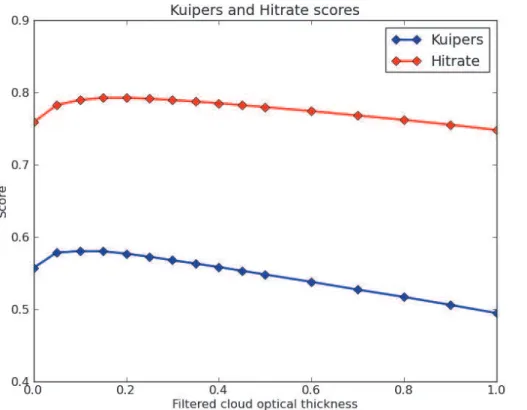
A way to estimate the cloud detection efficiency is to plot and analyse various statistical scores as a function of the CALIOP-filtered cloud optical thickness. For clarity, we re-peat that the filtering process means that whenever CALIOP-derived total cloud optical thickness in the column/FOV falls below a specific cloud optical thickness threshold we will treat the observation as if being cloud-free when calculating statistics. Figures 4–

15

6 show the results for all statistical parameters described in Sect. 3.3 based on all collocated orbits.

The basic mean error and RMS error quantities are shown together with the resulting total cloud fraction (i.e. percentage cloudy FOVs of all FOVs) in the CALIPSO-CALIOP dataset in Fig. 4. We notice that after filtering clouds having optical thicknesses up to

20

1.0, the total cloud fraction for CALIOP reduces from approximately 73 % to 50 %. At the same time the mean error changes from −14 % to ₊8 % and the RMS changes

from 47 % to 50 %. Based on mean error results alone one might conclude that the optimal agreement is reached after filtering all cloudy columns with optical thickness values below 0.35. The fact that mean errors become positive for higher filtered optical

25

(18)

AMTD

6, 1093–1141, 2013

dataset

Title Page

Tables Figures

◭ ◮

Back Close

Full Screen / Esc

Discussion

P

a

per

|

Dis

cussion

P

a

per

|

Discussion

P

a

per

|

Discussio

n

P

a

per

|

thickness thresholds only means that some cloudy CALIOP columns are now treated as being cloud-free even if they were detected successfully by CLARA-A1/PPS, thus giving a positive mean error. If comparing with Fig. 6 showing Hitrates and Kuiper’s skill scores, we see that the skill now peaks at slightly lower values of the filtered cloud optical thickness threshold, namely at about 0.2 for Hitrate and 0.1 for Kuiper’s skill

5

score. This shows that from these different statistical measures it is not easy to make a very clear conclusion about cloud detection limits.

However, results of Probabilities of Detection and False Alarm Ratios (hereafter de-noted POD and FAR) in Fig. 5 also reveal some further features of CLARA-A1/PPS results. These features are not evident in Fig. 4 or 6 and, in particular, they are not

10

directly related to how thin or thick clouds are. We first note that the FAR quantity for clear FOVs initially reduces rapidly with increasing value of the filtered cloud optical thickness. This is what we should expect if very thin cloud layers are not detected by CLARA-A1/PPS, i.e. scores would improve if also these CALIOP observations are treated as being cloud-free. Similarly, POD for cloudy conditions improves with

increas-15

ing values of filtered optical thickness. However, more serious is the observation that the FAR quantity for cloudy conditions amounts to 8 % initially for unfiltered CLARA-A1/PPS results. Thus, we seem to have a significant misclassification of clear FOVs labelled as cloudy which also explains why POD results for clear conditions are rela-tively far away from 100 % in the unfiltered mode. This shows that the cloud detection

20

e_fficiency cannot be judged solely from studies of how thin or thick clouds are. It is clear that there are also Earth surfaces that have appearances that resemble those of clouds regardless of whether clouds are thin or thick. The most obvious example is the case when interpreting a cold ground surface at night as being a cloud if us-ing an inappropriate value of the assumed ground surface temperature (i.e. beus-ing too

25

(19)

AMTD

6, 1093–1141, 2013

dataset

Title Page

Tables Figures

◭ ◮

Back Close

Full Screen / Esc

Discussion

P

a

per

|

Dis

cussion

P

a

per

|

Discussion

P

a

per

|

Discussio

n

P

a

per

|

type of misclassifications which could be interpreted as a constant bias in our results not related to the thickness of the clouds.

4.1.2 Results after excluding misclassified cloud-free surfaces

The most obvious way of trying to isolate the results depending mainly on the cloud optical thickness value of clouds would be to remove or ignore all cases being

misclas-5

sified as cloudy in the completely unfiltered mode. In other words, let us restore the cloudy CLARA-A1/PPS pixels in evidently cloud-free CALIOP FOVs to become clear. Thus, these 8 % of the cases in the FAR category for cloudy pixels in the unfiltered mode are now being treated as correctly classified as clear. Ideally, we should also try to exclude or ignore the oppositely misclassified cases, i.e. when clouds are

misclas-10

sified as clear regardless of their optical thickness (i.e. for non-separability reasons). However, these cases are not as easily identified as the cases of misclassified clear pixels. More clearly, they can occur at any cloud optical thickness meaning that these cases are inherently mixed with all the cases we actually aim at, namely those cases when cloud detection will clearly depend on the cloud optical thickness value. In that

15

sense these misclassifications exist as an almost constant bias in our results. They are best identified in Fig. 5 as explaining why the FAR_clearvalue is still high (20 %) even at the maximum filtered cloud optical thickness of 1.0. It means that in 20 % of all cases when CLARA-A1/PPS gives a cloud free result there are actually clouds in reality and they have cloud optical thickness values higher than 1.0. Further details on when these

20

misclassifications occur will be revealed in forthcoming Sects. 4.1.3 and 4.1.4.

The revised results for the statistical scores (after ignoring misclassified clear cases labelled as cloudy) are now shown in Figs. 7–9. We notice in Fig. 7 that now the mean error quantity does not reach the zero level until at a filtered cloud optical thickness of 0.7. This is a high value and indicates that the CLARA-A1/PPS cloud screening method

25

is generally rather cloud conservative. But it does not necessarily mean that the cloud detection limit is best described by this value of optical thickness. Rather we should use a quantity which is more uniquely decided by and dependent on the filtered cloud

(20)

AMTD

6, 1093–1141, 2013

dataset

Title Page

Tables Figures

◭ ◮

Back Close

Full Screen / Esc

Discussion

P

a

per

|

Dis

cussion

P

a

per

|

Discussion

P

a

per

|

Discussio

n

P

a

per

|

optical thickness. The two quantities that best fit this description seems to be POD for cloudy conditions and FAR for clear conditions. The first quantity improves with in-creasing filtered optical thicknesses until “all” clouds are detected. The fact that the POD_cloudysaturation level does not reach 100 % means that the difference with respect to the 100 % level represent all those cases where clouds remain undetected

regard-5

less of their cloud optical thickness. Similarly, the FAR for clear conditions behaves in the same way where the apparent convergence level defines the same misclassified cases (i.e. that portion of the CLARA-A1/PPS clear cases that actually are undetected clouds even for higher optical depths).

The significant increase at lower optical thicknesses than 0.7 of the POD quantity

10

for cloudy conditions and the corresponding decrease of the FAR quantity for clear conditions in Fig. 8 shows that much thinner clouds than what the mean error quantity indicates are indeed detected. A better value of the minimum optical thickness detected could then be suggested to be derived from the rate of change of the mentioned POD and FAR quantities for cloudy and clear conditions, respectively. The minimum optical

15

thickness to be determined would then be the value found when the improvement of these two quantities have slowed down or “saturated” (i.e. approaching constant or almost constant values). The interpretation of this value would be that at this cloud optical thickness all clouds are detected, unless other problems not related to how thick clouds are exists. For lower cloud optical thicknesses some clouds will be detected but

20

for very low optical thicknesses no clouds at all will be detected. Here, we will apply the following criteria for finding this cloud optical thickness limit:

δPOD_cloudy

δτ +

δ_FAR_clear

δτ

!

<1 % (9)

This means that we will interpret the cloud detection limit as the first (i.e. lowest) cloud optical thickness value where this inequality is fulfilled while checking for higher and

25

(21)

AMTD

6, 1093–1141, 2013

dataset

Title Page

Tables Figures

◭ ◮

Back Close

Full Screen / Esc

Discussion

P

a

per

|

Dis

cussion

P

a

per

|

Discussion

P

a

per

|

Discussio

n

P

a

per

|

the two quantities had reached almost constant values. Consequently, if applying this definition we get an overall cloud detection limit of optical thickness 0.35.

If comparing with Fig. 9 we see that this value is also relatively close to where the maximum of the Hitrate score occurs (although it is peaking at slightly lower optical thickness values). The Kuiper’s score does not really help us here. If remembering that

5

this score is a measure of how well cloudy and cloud-free situations are separated, it is clear that this will now occur in the unfiltered case (after having removed all obviously misclassified cloudy cases).

4.1.3 Results subdivided into day and night portions

Since the overall results include results from both illuminated and dark conditions, an

10

interesting aspect is to study what happens if we look at both conditions separately. Basically, it means that we look at the impact of having access to visible spectral chan-nels (i.e. information on reflected sunlight) or not. Figures 10–12 show corresponding results for all statistical scores at day and at night (as defined in Sect. 3.3). All figures show convincingly how cloud detection e_fficiency degrades for night-time conditions.

15

For example, in Fig. 10 we see that while the mean error reaches the zero level already at cloud optical thickness 0.2 during day it never reaches this level at night (i.e. remains negative). It is clear that a large fraction of all clouds are not detected at night, even at large cloud optical thicknesses. This is also well illustrated in Fig. 11 with decreasing POD_cloudy and increasing FAR_clear at night (i.e. FAR_clear at filtered cloud optical

thick-20

ness of 1.0 increases from about 10 % during day to about 25 % during night). Skill scores in Fig. 12 also show significantly better results during day compared to during night. Thus, the availability of information in the visible and short-wave infrared AVHRR channels appears to be quite important for the success of cloud detection.

Somewhat surprising, the derived value of the minimum cloud detection limit

(accord-25

ing to Eq. 9) is found at cloud optical thickness 0.3 for both day and night conditions. Thus, the sensitivity to the filtered cloud optical thickness is relatively unchanged even if much fewer clouds are detected at night. We conclude that this must be explained

(22)

AMTD

6, 1093–1141, 2013

dataset

Title Page

Tables Figures

◭ ◮

Back Close

Full Screen / Esc

Discussion

P

a

per

|

Dis

cussion

P

a

per

|

Discussion

P

a

per

|

Discussio

n

P

a

per

|

by the increase in frequency of cases when clouds are completely missed at night (as indicated by the high FAR_clear value at night). Thus, we are facing more general non-separability conditions of clouds and Earth surfaces at night and this has nothing to do with how thick clouds are. The fact that the overall cloud detection limit was esti-mated to be at cloud optical thickness 0.35 in Sect. 4.1.2 (i.e. higher than the derived

5

value for either day or night) indicates that conditions must be especially problematic at twilight conditions. Hence, the cloud detection limit is found to lie at a cloud opti-cal thickness of 0.45 for twilight conditions. From Fig. 13, showing the POD and FAR quantities at twilight conditions, we conclude that this is explained by the rather slow increase in POD_cloudyand the corresponding slow decrease of FAR_clear for increasing

10

filtered cloud optical thicknesses. Thus, at twilight we still miss a substantial fraction of optically thick clouds (more or less the same fraction as during night) but now we also face increasing difficulties in detecting thinner clouds.

4.1.4 Global results subdivided into regions

Let us now look at the geographical variations of the validation results. This might

15

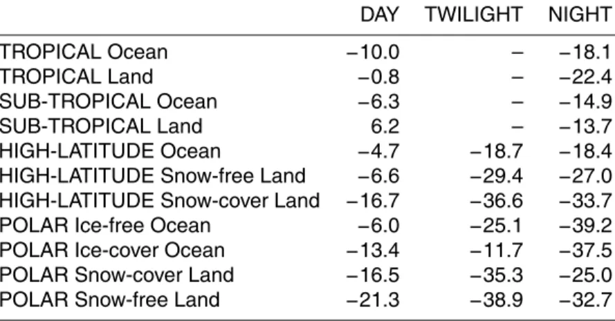
shed some further light on actually where we encounter the static problems of mis-classified clear or mismis-classified cloudy conditions, i.e. those misclassifications that are not depending on existing clouds’ optical thickness. If first considering the unfiltered CALIPSO results, we will investigate if there are specific regions where misclassifica-tions of cloud-free areas occur (i.e. explaining the 8 % of CLARA-A1/PPS misclassified

20

clear cases mentioned in Sect. 4.1.2). These results are summarised for the mean er-ror quantity in Table 3 for latitudinal bands defined in Table 2, for day, twilight and night categories and for land and ocean surfaces. We restrict the description to the mean error quantity since by this detailed sub-division of results the number of samples per category is sometimes too small to enable a proper estimation of all the statistical

25

(23)

AMTD

6, 1093–1141, 2013

dataset

Title Page

Tables Figures

◭ ◮

Back Close

Full Screen / Esc

Discussion

P

a

per

|

Dis

cussion

P

a

per

|

Discussion

P

a

per

|

Discussio

n

P

a

per

|

layers. However, one of the categories actually showing some overestimation (+6.2 %) is the category sub-tropical land. Near-zero results are also presented for the tropical land category. Further visual inspection of results revealed that misclassifications of clear conditions mainly occur over semi-arid land areas, i.e. in the zone where desert regions change from being pure desert to being partly vegetation-covered. Thus,

mis-5

classifications do not occur over pure desert areas but where we have a seasonal transition from near-desert conditions to tropical vegetated conditions.

Table 4 shows results where we treat all CALIOP-detected clouds with cloud optical thicknesses lower than 0.35 as non-existent (i.e. as cloud-free cases). We notice that for the day category we now get dominantly positive values, i.e. we normally detect

10

some clouds that are thinner than optical thickness 0.35. However, the overestimation is now quite excessive for categories sub-tropical land and tropical land which even further emphasizes the misclassification problems encountered here. Some positive values are also seen at night over sub-tropical and tropical categories but otherwise we have dominantly negative results for night and twilight categories which is in line

15

with the results discussed previously in Sect. 4.1.3. For these categories, we obviously do not detect a substantial fraction of all clouds regardless of their optical thickness. This occurs mainly in the Polar regions but also during dark and snow-covered periods over high latitude regions.

4.2 Cloud top height results 20

Results from the evaluation of cloud top height retrievals (following the method de-scribed in Sect. 3.4) are presented in Table 5. Results are here also compared with cases where we did not apply any filtering of very thin cloud layers and where we also always compared with the cloud top boundary for the uppermost CALIOP cloud layer (instead of the mid-layer value).

25

It is obvious from Table 5 that the chosen validation methodology has a tremendous impact on the achived results. If including all thin cloud layers and if comparing with uppermost cloud boundary, a substantial underestimation of cloud top heights is found

(24)

AMTD

6, 1093–1141, 2013

dataset

Title Page

Tables Figures

◭ ◮

Back Close

Full Screen / Esc

Discussion

P

a

per

|

Dis

cussion

P

a

per

|

Discussion

P

a

per

|

Discussio

n

P

a

per

|

(on the average more than 2.5 km). If instead taking into account the cloud detection limit and trying to represent clouds with a more radiatively relevant height results im-prove drastically (overall bias of−274 m). If filtering with the optical thickness value of

0.5 the bias almost disappears. However, if taking advantage of that the CALIOP cloud layer description in the Vertical Feature Mask product also includes a sub-division into

5

categories low-level, medium-level and high-level clouds following the ISCCP definition, we notice that the small bias is largely a result of the sum of a large underestimation of high-level cloud tops (−1769 m) and a large overestimation of low-level cloud tops

(₊1137 m). Thus, there seems to be di_fferent behaviour of high-level clouds and low-level clouds. The low-low-level boundary layer cloud problem is the same as being reported

10

previously for MODIS cloud top products (Menzel et al., 2008). For CLARA-A1/PPS it can be explained as a problem with the reference atmospheric temperature profile taken from NWP analyses (here, ERA-Interim). For boundary layer clouds trapped in a temperature inversion, the reference profile is not detailed enough (i.e. too weak in-version which is partly due to the mismatch between pixel and NWP grid resolution)

15

leading to an overestimation of the cloud top height. A typical example of when this occurs can be seen in Fig. 3 between track positions 7000 and 8000.

The underestimation of high-level clouds reflects the problem of how to define the radiatively efficient cloud top height for thin and multiple cloud layers for an infrared channel of a passive imager. CALIOP measurements have also revealed the frequent

20

existence of surprisingly thick (geometrically) single cloud layers which are optically very thin. Good examples of this are found in Fig. 3 at track positions 2400, 4000 and 6500. The use of a mid-layer representation of such a cloud layer is apparently still inadequate. Currently, CLARA-A1/PPS retrievals underestimate the height for all high-level clouds substantially even if the method of applying cloud filtering of the thinnest

25

(25)

AMTD

6, 1093–1141, 2013

dataset

Title Page

Tables Figures

◭ ◮

Back Close

Full Screen / Esc

Discussion

P

a

per

|

Dis

cussion

P

a

per

|

Discussion

P

a

per

|

Discussio

n

P

a

per

|

The corresponding integrated cloud optical thickness should obviously be larger than the estimated detection limit of 0.35. But even if we cannot determine this value exactly, the systematic use of a stipulated value (e.g. optical thickness 1.0) could be valuable in the evaluation of different and upgraded cloud height retrieval methods in the future.

5 Conclusions 5

This study investigated the optimal validation methodology to be used when evaluating cloud retrievals from passive imagers for taking full advantage of the measurements provided by the active cloud lidar CALIOP carried by the CALIPSO satellite. Some inconsistencies of the current CALIOP datasets were identified and a method for mit-igating the influence of those was proposed. The method was applied for evaluating

10

a sub-set (covering the years 2006–2009) of the CMSAF CLARA-A1 dataset derived from historical global AVHRR data. It was demonstrated how the CALIOP-provided information of cloud presence and cloud optical thickness can be used to delineate the current cloud detection limitations of the methods used to compile the CLARA-A1 dataset. Although the cloud detection capability does vary with time of day and with

15

the geographical environment, an overall cloud detection limit was estimated at a cloud optical thickness of 0.35. It means that at this cloud optical thickness most cloud lay-ers are being detected. Thinner clouds are detected but at decreasing e_fficiency with smaller cloud optical thickness. The diurnal variation showed that the detection limit is close to 0.3 both day and night while conditions are deteriorating considerably at

20

twilight conditions when the cloud detection limit is estimated to 0.45.

The study also revealed that there is a substantial fraction of cases where cloud detection results are not depending at all on the thickness of existing clouds. In other words, there are cases where clouds are either completely missed or falsely identified. This explains why the probability of detecting clouds is limited to about 90 % during day

25

but as low as 75–80 % during night and twilight conditions. Daytime misclassifications of semi-arid sub-tropical and tropical land surfaces as clouds were identified, as well

(26)

AMTD

6, 1093–1141, 2013

dataset

Title Page

Tables Figures

◭ ◮

Back Close

Full Screen / Esc

Discussion

P

a

per

|

Dis

cussion

P

a

per

|

Discussion

P

a

per

|

Discussio

n

P

a

per

|

as a substantial amount of missed clouds in the Polar regions during the Polar win-ter. Both deficiencies are well understood and reflect major challenges for most cloud retrieval schemes using data from passive imagery. The daytime problem is linked to the fundamental difference in the cloud-free spectral appearance of desert surfaces and tropical forested surfaces. While cloud screening seems to work well over both

5

mentioned surfaces, problems arise in the transition zone between them where the appearance also changes seasonally. The current methodology has an inappropriate description of this transition zone and the associated temporal changes of its surface appearance (i.e. a static climatology is used). Thus, an improved methodology must address this limitation in the future.

10

The underestimation of cloudiness at high latitudes and especially during winter con-ditions is linked to another well-known problem for all cloud screening methods applied to passive imagery. It occurs when there is no distinct temperature difference between clouds and the underlying surface. The situation becomes even worse if the tempera-ture di_fference is also reversed (i.e. if clouds are warmer than the surface) which is a

fre-15

quent feature in the polar winter. Also, when ground temperatures becomes extremely cold (like over the Antarctic plateau in the polar winter) the radiometric accuracy of the AVHRR measurement is not any longer accurate enough for estimating the brightness temperature difference between infrared channels; a quantity that is heavily used by many cloud screening methods. Altogether, this leads for CLARA-A1 to a substantial

20

underestimation of cloudiness over Polar regions in the polar winter and also during night and twilight conditions at high latitudes. Notice that even if this problem is com-mon to most cloud screening methods applied in the Polar region, the achieved results may di_ffer depending on the actual method. For some methods like CLARA-A1/PPS the problems are manifested as missed clouds while for other methods it could as well

25

lead to overestimated cloudiness (misclassified cold cloud-free surfaces).

(27)

AMTD

6, 1093–1141, 2013

dataset

Title Page

Tables Figures

◭ ◮

Back Close

Full Screen / Esc

Discussion

P

a

per

|

Dis

cussion

P

a

per

|

Discussion

P

a

per

|

Discussio

n

P

a

per

|

single-layer clouds or too thin uppermost cloud layers. Results were shown to differ substantially depending on whether the cloud top boundary was defined as the upper-most CALIOP-derived cloud layer boundary or as the mid-level (i.e. the mean of cloud base and cloud top) of the corresponding CALIOP-observed cloud layer. The latter def-inition gives a height that is closer to the radiatively e_fficient level of the cloud which

5

better resembles the level that is normally retrieved from passive imagery.

When using the latter approach a relatively small total cloud top height bias of−274 m

was found. This can be compared to the cloud top height bias of −2762 m for the

default method based on the uppermost cloud boundary and including all thin clouds. However, even after using the more realistic radiatively efficient level approximation it

10

is clear that large underestimations of high-level cloud top heights and overestimations of low-level cloud top heights exist which has to be addressed in a future reprocessing of the dataset.

In conclusion, we have demonstrated how CALIPSO-CALIOP results can be used to carry out a very detailed examination of cloud retrieval results from passive imagers.

15

Results presented here are not entirely surprising or unexpected but they are given with unprecedented detail. Although the current CALIOP datasets show some internal inconsistencies depending on the FOV resolution, we have shown how these can be mitigated to construct a more reasonable validation reference. As such, we believe that its value is unprecedented and that it can be used as an invaluable reference for the

20

evaluation of any cloud retrieval scheme based on data from passive imagers. In par-ticular, we believe that even beyond the lifetime of the CALIPSO satellite, the extracted subset of collocated NOAA-18 and CALIPSO-CALIOP observations might serve as a benchmarking dataset for the testing of various AVHRR-based cloud retrieval meth-ods. For the planned future upgrades of the CLARA-A1 dataset, the idea is to use the

25

currently collected CALIPSO dataset in exactly this way. There is a limitation in that it is based exclusively on afternoon-orbit NOAA-18 data but we believe that it can be complemented with a limited set of morning-orbit data from satellites carrying the mod-ified AVHRR instrument with the additional 1.6 µm channel. Although, for the latter the