ACPD
15, 8687–8770, 2015Tropospheric chemistry reanalysis
K. Miyazaki et al.
Title Page
Abstract Introduction
Conclusions References
Tables Figures
◭ ◮
◭ ◮
Back Close
Full Screen / Esc
Printer-friendly Version Interactive Discussion
Discussion
P
a
per
|
Discussion
P
a
per
|
Discussion
P
a
per
|
Discussion
P
a
per
|
Atmos. Chem. Phys. Discuss., 15, 8687–8770, 2015 www.atmos-chem-phys-discuss.net/15/8687/2015/ doi:10.5194/acpd-15-8687-2015
© Author(s) 2015. CC Attribution 3.0 License.
This discussion paper is/has been under review for the journal Atmospheric Chemistry and Physics (ACP). Please refer to the corresponding final paper in ACP if available.
A tropospheric chemistry reanalysis for
the years 2005–2012 based on an
assimilation of OMI, MLS, TES and
MOPITT satellite data
K. Miyazaki1, H. J. Eskes2, and K. Sudo3
1
Japan Agency for Marine-Earth Science and Technology, Yokohama 236-0001, Japan 2
Royal Netherlands Meteorological Institute (KNMI), Wilhelminalaan 10, 3732 GK, De Bilt, the Netherlands
3
Graduate School of Environmental Studies, Nagoya University, Nagoya, Japan
Received: 19 February 2015 – Accepted: 13 March 2015 – Published: 24 March 2015
Correspondence to: K. Miyazaki (kmiyazaki@jamstec.go.jp)
ACPD
15, 8687–8770, 2015Tropospheric chemistry reanalysis
K. Miyazaki et al.
Title Page
Abstract Introduction
Conclusions References
Tables Figures
◭ ◮
◭ ◮
Back Close
Full Screen / Esc
Printer-friendly Version Interactive Discussion
Discussion
P
a
per
|
Discussion
P
a
per
|
Discussion
P
a
per
|
Discussion
P
a
per
|
Abstract
We present the results from an eight-year tropospheric chemistry reanalysis for the period 2005–2012 obtained by assimilating multiple retrieval data sets from the OMI, MLS, TES, and MOPITT satellite instruments. The reanalysis calculation was con-ducted using a global chemical transport model and an ensemble Kalman filter tech-5
nique that simultaneously optimises the chemical concentrations of various species and emissions of several precursors. The optimisation of both the concentration and
the emission fields is an efficient method to correct the entire tropospheric profile and
its year-to-year variations, and to adjust various tracers chemically linked to the species assimilated. Comparisons against independent aircraft, satellite, and ozonesonde ob-10
servations demonstrate the quality of the analysed O3, NO2, and CO concentrations on
regional and global scales and for both seasonal and year-to-year variations from the lower troposphere to the lower stratosphere. The data assimilation statistics imply per-sistent reduction of model error and improved representation of emission variability, but also show that discontinuities in the availability of the measurements lead to a degra-15
dation of the reanalysis. The decrease in the number of assimilated measurements
increased the ozonesonde minus analysis difference after 2010 and caused spurious
variations in the estimated emissions. The Northern/Southern Hemisphere OH ratio was modified considerably due to the multiple species assimilation and became closer to an observational estimate, which played an important role in propagating observa-20
tional information among various chemical fields and affected the emission estimates.
The consistent concentration and emission products provide unique information on year-to-year variations of the atmospheric environment.
1 Introduction
Long-term records of the tropospheric composition of gases such as ozone (O3),
car-25
ACPD
15, 8687–8770, 2015Tropospheric chemistry reanalysis
K. Miyazaki et al.
Title Page
Abstract Introduction
Conclusions References
Tables Figures
◭ ◮
◭ ◮
Back Close
Full Screen / Esc
Printer-friendly Version Interactive Discussion
Discussion
P
a
per
|
Discussion
P
a
per
|
Discussion
P
a
per
|
Discussion
P
a
per
|
changes in tropospheric chemistry and human activity and consequences for the at-mospheric environment and climate change (HTAP, 2010; IPCC, 2013). Satellite in-struments provide observations of the global distributions of tropospheric
composi-tion. For example, measurements of tropospheric O3 have been retrieved using the
Tropospheric Emission Spectrometer (TES) since 2004 (Beer, 2006) and by the In-5
frared Atmospheric Sounding Interferometer (IASI) since 2007 (Coman et al., 2012).
Tropospheric NO2 column concentrations have been retrieved by the Ozone
Monitor-ing Instrument (OMI) since 2004 (Levelt et al., 2006), ScannMonitor-ing ImagMonitor-ing Absorption Spectrometer for Atmospheric Cartography (SCIAMACHY) from 2002–2012 (Bovens-mann et al., 1999), Global Ozone Monitoring Experiment (GOME) from 1996–2003, 10
and GOME-2 since 2007 (Callies et al., 2000). The availability of satellite-derived mea-surements of various chemical species has prompted increasing interest to develop methods for combining these sources of satellite observational information, for stud-ies of long-term variations within the atmospheric environment and for improving the estimates of emissions sources (Inness et al., 2013; Streets et al., 2013).
15
Combining measurements of O3, CO and NOxin the atmosphere puts constraints on
the concentration of OH, the main radical responsible for the removal of pollution from the atmosphere and determining the lifetime of many chemicals (Levy, 1971; Logan et al., 1981; Thompson, 1992). At the same time the combined use provides
con-straints on different sources of surface emissions and production of NOx by lightning
20
(LNOx) (e.g., Martin et al., 2007; Miyazaki et al., 2014). The information that may be
obtained from a combined use of multiple satellite datasets without involving a model is
limited, related to differing vertical sensitivity profiles, different overpass times, and
mis-matches in spatial and temporal coverage between the instruments, as well as missing information on the chemical regime and origin of the air masses.
25
Data assimilation is the technique for combining different observational data sets with
ACPD
15, 8687–8770, 2015Tropospheric chemistry reanalysis
K. Miyazaki et al.
Title Page
Abstract Introduction
Conclusions References
Tables Figures
◭ ◮
◭ ◮
Back Close
Full Screen / Esc
Printer-friendly Version Interactive Discussion
Discussion
P
a
per
|
Discussion
P
a
per
|
Discussion
P
a
per
|
Discussion
P
a
per
|
measurements and propagates it, in time and space, from a limited number of ob-served species to a wide range of chemical components to provide global fields that are physically and chemically consistent and in agreement with the observations. Vari-ous studies have demonstrated the capability of data assimilation techniques regarding the analysis of chemical species in the troposphere and stratosphere.
5
Assimilation of satellite limb measurements for O3profiles and nadir measurements
for O3columns have been used to study O3variations in the stratosphere and the
up-per troposphere (e.g., Stajner and Wargan, 2004; Jackson, 2007; Stajner et al., 2008; Wargan et al., 2010; Flemming et al., 2011; Barre et al., 2013; Emili et al., 2014).
Long-term integrated data sets of stratospheric O3 have been produced by several studies
10
by combining multiple satellite retrieval datasets (e.g., Kiesewetter et al., 2010; Van der A et al., 2010). The assimilation of satellite observations has been also applied
to investigate global variations in the tropospheric composition of gases such as O3
and CO (e.g., Parrington et al., 2009; Coman et al., 2012; Miyazaki et al., 2012b). For providing long-term integrated data of tropospheric composition, as a pioneer study, 15
Inness et al. (2013) performed an eight-year reanalysis of tropospheric chemistry for 2003–2010 using an advanced data assimilation system. They included atmospheric
concentrations of O3, CO, NOx, and formaldehyde (CH2O) as the forecast model
vari-ables in the integrated forecasting system with modules for atmospheric composition
(C-IFS), and they demonstrated improved O3and CO profiles for the free troposphere.
20
They also highlighted biases remaining in the lower troposphere associated with fixed surface emissions, which are not adjusted in the 4D-Var assimilation scheme presented by Inness et al. (2013).
Currently available bottom-up inventories of emissions contain large uncertainties, mainly because of inaccurate activity rates and emission factors for each category and 25
poor representation of their seasonal and interannual variations (e.g., Jaeglé et al., 2005; Xiao et al., 2010; Reuter et al., 2014). Top-down inverse approaches using satel-lite retrievals have been applied to obtain optimised emissions of CO (e.g. Kopacz et al.,
ACPD
15, 8687–8770, 2015Tropospheric chemistry reanalysis
K. Miyazaki et al.
Title Page
Abstract Introduction
Conclusions References
Tables Figures
◭ ◮
◭ ◮
Back Close
Full Screen / Esc
Printer-friendly Version Interactive Discussion
Discussion
P
a
per
|
Discussion
P
a
per
|
Discussion
P
a
per
|
Discussion
P
a
per
|
2012a; Mijling et al., 2013), by minimising the differences between observed and
sim-ulated concentrations, as summarised by Streets et al. (2013). In addition to surface
emissions, the improved representations of LNOx sources are important for a
realis-tic representation of O3 formation and chemical processes in the upper troposphere
(Schumann and Huntrieser, 2007; Miyazaki et al., 2014). 5
The simultaneous adjustment of emissions and concentrations of various species is a new development in tropospheric chemical reanalysis and long-term emissions anal-ysis. Miyazaki et al. (2012b) developed a data assimilation system, called CHASER-DAS, for the simultaneous optimization of the atmospheric concentration of various
trace gases, together with an optimization of the surface emissions of NOx and CO,
10
and the LNOxsources, while taking their complex chemical interactions into account, as
represented by the CHASER chemistry-transport model. Within the simultaneous opti-misation framework, the analysis adjustment of atmospheric concentrations of chemi-cally related species has the potential to improve the emission inversion (Miyazaki and Eskes, 2013; Miyazaki et al., 2014). This was compared with an emission inversion 15
based on measurements from one species alone, where uncertainties in the model
chemistry affect the quality of the emission source estimates. In addition, the improved
estimates of emissions benefit the atmospheric concentration analysis through a re-duction in model forecast error. The simultaneous adjustment of the emissions and the concentrations is therefore a powerful approach to optimize all aspects of the chemical 20
system influencing tropospheric O3(Miyazaki et al., 2012b).
In this study, we present a tropospheric chemistry reanalysis data set for the eight-year period from 2005 to 2012 using CHASER-DAS. This reanalysis is produced with the CHASER-DAS system introduced in Miyazaki et al. (2012b). The system uses the ensemble Kalman filter (EnKF) assimilation technique and assimilates Microwave Limb 25
ACPD
15, 8687–8770, 2015Tropospheric chemistry reanalysis
K. Miyazaki et al.
Title Page
Abstract Introduction
Conclusions References
Tables Figures
◭ ◮
◭ ◮
Back Close
Full Screen / Esc
Printer-friendly Version Interactive Discussion
Discussion
P
a
per
|
Discussion
P
a
per
|
Discussion
P
a
per
|
Discussion
P
a
per
|
information for various research topics related to the inter-annual variability of the at-mospheric environment and short-term trends.
The remainder of this paper is structured as follows. Section 2 describes the obser-vations used for the assimilation and validation. Section 3 introduces the data assim-ilation system and Sect. 4 evaluates the reanalysis performance based on analyses 5
of data assimilation statistics. Section 5 presents comparisons against independent observations. Section 6 describes the emission source estimation results. Section 7,
which discusses possible errors in the reanalysis data and offers thoughts on future
developments, is followed by the conclusions in Sect. 8.
2 Data assimilation system
10
The CHASER-DAS system (Miyazaki et al., 2012a, b, 2014; Miyazaki and Eskes, 2013) has been developed based on an EnKF approach and a global chemical transport model called CHASER. The data assimilation settings used for the reanalysis calcula-tion are mostly the same as in Miyazaki et al. (2014), but the calculacalcula-tion was extended to cover the eight years from 2005–2012, and several updates were applied to the a pri-15
ori and state vector settings. Brief descriptions of the forecast model, data assimilation approach, and experimental settings are presented below.
2.1 Forecast model
The CHASER model (Sudo et al., 2002, 2007) was used as a forecast model. It has
so-called T42 horizontal resolution (2.8◦) and 32 vertical levels from the surface to
20
ACPD
15, 8687–8770, 2015Tropospheric chemistry reanalysis
K. Miyazaki et al.
Title Page
Abstract Introduction
Conclusions References
Tables Figures
◭ ◮
◭ ◮
Back Close
Full Screen / Esc
Printer-friendly Version Interactive Discussion
Discussion
P
a
per
|
Discussion
P
a
per
|
Discussion
P
a
per
|
Discussion
P
a
per
|
Model Intercomparison Project II (NCEP-DOE/AMIP-II) reanalysis (Kanamitsu et al., 2002) at every time step of the AGCM to reproduce past meteorological fields. The nudged AGCM enabled us to perform CHASER calculations that included short-term atmospheric variations and parameterised transport processes by sub-grid-scale con-vection and boundary layer mixing.
5
The a priori value for surface emissions of NOxand CO were obtained from
bottom-up emission inventories. Anthropogenic NOx and CO emissions were obtained from
the Emission Database for Global Atmospheric Research (EDGAR) version 4.2. Emis-sions from biomass burning are based on the monthly Global Fire EmisEmis-sions Database (GFED) version 3.1 (van der Werf et al., 2010). Emissions from soils are based 10
on monthly mean Global Emissions Inventory Activity (GEIA) (Graedel et al., 1993). EDGAR version 4.2 was not available after 2008 at the time the reanalysis was started; therefore, the emissions for 2008 were used in the calculations for 2009–2012. GFED 3.1 was not available for 2012 and thus, the emissions averaged over 2005–2011
were used in the calculation for 2012. For surface NOx emissions, a diurnal variability
15
scheme developed by Miyazaki et al. (2012) was applied depending on the dominant category for each area: anthropogenic, biogenic, and soil emissions.
For the calculation of a priori LNOxemissions, the global distribution of the flash rate
was parameterised in CHASER for convective clouds based on the relation between lightning activity and cloud top height (Price and Rind, 1992). To obtain a realistic es-20
timate of the global annual total flash occurrence, a tuning factor was applied for the global total frequency, which is independent of the lightning adjustment in the assimi-lation. The global distribution of the total flash rate is generally reproduced well by the model in comparison with the observations, except for overestimations over northern South America and underestimations over both Central Africa and most of the oceanic 25
ACPD
15, 8687–8770, 2015Tropospheric chemistry reanalysis
K. Miyazaki et al.
Title Page
Abstract Introduction
Conclusions References
Tables Figures
◭ ◮
◭ ◮
Back Close
Full Screen / Esc
Printer-friendly Version Interactive Discussion
Discussion
P
a
per
|
Discussion
P
a
per
|
Discussion
P
a
per
|
Discussion
P
a
per
|
2.2 Data assimilation technique
The data assimilation technique employed is an EnKF approach, i.e., a local ensemble transform Kalman filter (LETKF, Hunt et al., 2007) based on the ensemble square root filter (SRF) method, which uses an ensemble forecast to estimate the background error covariance matrix. The covariance matrices of the observation error and background 5
error determine the relative weights given to the observation and the background in the analysis. The advantage of the EnKF over 4D-VAR is its simple implementation for complicated systems such as CTMs. The LETKF has conceptual and computational advantages over the original EnKF. First, the analysis is performed locally in space and time, which reduces sampling errors caused by limited ensemble size. Second, the 10
analyses performed independently for different grid points allow parallel computations
to be performed that reduce the computational cost. These advantages are important in the chemical reanalysis calculation because of the many analysis steps included in the eight-year reanalysis run and the large state vector size used for the multiple states optimisation (cf., Sects. 2.3 and 2.7).
15
The forecast and analysis steps are described briefly below.
2.2.1 The forecast step
The background ensemble mean xb and its perturbation Xb are obtained from the
evolution of each ensemble member using the forecast model,
xb=1
k
k
X
i=1
xb
i; X
b
i =x
b
i −xb. (1)
20
Xbis an N×k matrix, where N indicates the system dimension andk represents the
ensemble size. Based on the assumption that background ensemble perturbationsXb
sample the forecast errors, the background error covariance is estimated as follows:
ACPD
15, 8687–8770, 2015Tropospheric chemistry reanalysis
K. Miyazaki et al.
Title Page
Abstract Introduction
Conclusions References
Tables Figures
◭ ◮
◭ ◮
Back Close
Full Screen / Esc
Printer-friendly Version Interactive Discussion
Discussion
P
a
per
|
Discussion
P
a
per
|
Discussion
P
a
per
|
Discussion
P
a
per
|
An ensemble of background vectors ybi and an ensemble of background
perturba-tions in the observation spaceYbare estimated using the observation operatorH (cf.,
Sect. 2.5):
ybi =Hxbi;Yb=ybi −yb. (3)
2.2.2 The analysis step
5
The analysis ensemble mean is obtained by updating the background ensemble mean:
xa=xb+XbPea(Yb)TR−1
(yo−yb), (4)
whereyo represents the observation vector, R is thep×p observation error
covari-ance, andp indicates the number of observations. The observation error information
is obtained for each retrieval (cf., Sect. 2.6), wherePeais thek×k local analysis error
10
covariance in the ensemble space:
e
Pa=
(k−1)I
1+ ∆ + Y
bT
R−1Yb
−1
. (5)
A covariance inflation factor (∆ =6 %) was applied to inflate the forecast error
co-variance at each analysis step. The inflation is used to prevent an underestimation of background error covariance and resultant filter divergence caused by model errors 15
and sampling errors. The estimation of thePea matrix does not require any calculation
of large vectors or matrices withN dimensions in the LETKF algorithm.
The new analysis ensemble perturbation matrix in the model space (Xa) is obtained
by transforming the background ensembleXbwithPea:
Xa=Xbh(k−1)Peai 1/2
. (6)
20
ACPD
15, 8687–8770, 2015Tropospheric chemistry reanalysis
K. Miyazaki et al.
Title Page
Abstract Introduction
Conclusions References
Tables Figures
◭ ◮
◭ ◮
Back Close
Full Screen / Esc
Printer-friendly Version Interactive Discussion
Discussion
P
a
per
|
Discussion
P
a
per
|
Discussion
P
a
per
|
Discussion
P
a
per
|
2.3 State vector
The state vector for the reanalysis calculation is chosen to optimise the tropospheric chemical system and to improve the reanalysis performance. The state vector used in
the reanalysis includes several emission sources (surface emissions of NOx and CO,
and LNOx sources) as well as the predicted concentrations of 35 chemical species,
5
in the form of a scaling factor for each surface grid cell for the complete NOx and CO
emissions at the surface (not for individual sectors) and for each production rate
pro-file of the LNOx sources. Perturbations obtained by adding these model parameters
into the state vector introduced an ensemble spread of chemical concentrations and emissions in the forecast step. The background error correlations, estimated from the 10
ensemble model simulations at each analysis step, determine the relationship between the concentrations and emissions of related species, which can reflect daily, seasonal, interannual, and geographical variations in transport and chemical reactions. The emis-sion sources were optimised at every analysis step throughout the reanalysis period. The initial bias in the a priori emissions can be reduced gradually through the data 15
assimilation cycle.
2.4 Covariance localisation
The EnKF approaches always have the problem of introducing unrealistic long dis-tance error correlations because of the limited number of ensemble members. During the reanalysis calculation, such spurious correlations lead to errors in the fields that 20
may accumulate and will influence the reanalysis quality in a negative way. In order to improve the filter performance, the covariance among non- or weakly related variables in the state vector is set to zero based on sensitivity calculation results, as in Miyazaki
et al. (2012b). The analysis of surface emissions of NOx and CO allowed for error
correlations with OMI NO2 and MOPITT CO data, while those with other data were
25
neglected. For the LNOxsources, covariances with MOPITT CO data were neglected.
ACPD
15, 8687–8770, 2015Tropospheric chemistry reanalysis
K. Miyazaki et al.
Title Page
Abstract Introduction
Conclusions References
Tables Figures
◭ ◮
◭ ◮
Back Close
Full Screen / Esc
Printer-friendly Version Interactive Discussion
Discussion
P
a
per
|
Discussion
P
a
per
|
Discussion
P
a
per
|
Discussion
P
a
per
|
MLS O3 and HNO3 observations. Different from the study of Miyazaki et al. (2012b),
concentrations of non-methane hydrocarbons (NMHC) were not optimised in the re-analysis. The assimilation of MOPITT CO data led to concentrations of NMHC that increased to unrealistic values during the reanalysis, likely associated with too much chemical destruction of CO (cf., Sect. 7.4.2).
5
Covariance localization was also applied to avoid the influence of remote observa-tions, which is described in Sect. 2.7.
2.5 Observation operator
The observation operator (H) includes the spatial interpolation operator (S), a priori
profile (xapriori), and averaging kernel (A), which maps the model fields (x
b
) into retrieval 10
space (yb) thereby accounting for the vertical averaging implicit in the observations, as
follows:
yb=H(xb)=xapriori+A(S(xb)−xapriori), (7)
wherexbis theN-dimensional state vector andybis thep-dimensional model
equiva-lent of the observational vector. The averaging kernel (A) defines the vertical sensitivity 15
profile of the satellite retrievals and removes the dependence of the analysis on the re-trieval a-priori profile (Eskes and Boersma, 2003).
2.6 Observation error
The observation error provided in the retrieval data products includes contributions from the smoothing errors, model parameter errors, forward model errors, geophysical 20
noise, and instrument errors. In addition, a representativeness error was added for the
OMI NO2and MOPITT CO observations to account for the spatial resolution differences
ACPD
15, 8687–8770, 2015Tropospheric chemistry reanalysis
K. Miyazaki et al.
Title Page
Abstract Introduction
Conclusions References
Tables Figures
◭ ◮
◭ ◮
Back Close
Full Screen / Esc
Printer-friendly Version Interactive Discussion
Discussion
P
a
per
|
Discussion
P
a
per
|
Discussion
P
a
per
|
Discussion
P
a
per
|
error correlation of 15 % among the individual satellite observations within a model grid cell.
2.7 Reanalysis settings
Because a single continuous calculation for eight years requires a long computational time, we parallelised the reanalysis calculation. Eight series of one-year calculations 5
were conducted for 2005–2012, with a two-month spin-up starting from the 1 November of the previous year, whereas each one-year run was parallelized on 16 processors.
The two-month spin-up removed the differences in the analysis between the different
time series, providing a continuous eight-year data set. Because of distinct diurnal variations in the tropospheric chemical system, the data assimilation cycle was set 10
to be short (i.e., 120 min) to reduce sampling errors. The emission and concentration fields were analysed and updated at every analysis step.
In the reanalysis calculation the ensemble size was set to 30, which is somewhat smaller than the 48 members used in our previous studies. A smaller ensemble size reduces computational cost, but slightly degrades analysis performance, as quantified 15
in Miyazaki et al. (2012b). The horizontal localisation scaleLwas set to 450 km for NOx
emissions and 600 km for CO emissions, LNOx, and the concentrations. These choices
are based on sensitivity experiments (Miyazaki et al., 2012b), for which the influence of an observation was set to zero when the distance between the observation and
analysis point was larger than 2L×
q
10/3.
20
The a priori error was set to 40 % for surface emissions of NOx and CO and 60 %
for LNOx sources, but a model error term was not implemented for emissions during
the forecast. To prevent covariance underestimation and maintain emission variabil-ity during the long-term reanalysis calculation, we applied covariance inflation to the emission source factors in the analysis step, i.e., model error is implemented through 25
ACPD
15, 8687–8770, 2015Tropospheric chemistry reanalysis
K. Miyazaki et al.
Title Page
Abstract Introduction
Conclusions References
Tables Figures
◭ ◮
◭ ◮
Back Close
Full Screen / Esc
Printer-friendly Version Interactive Discussion
Discussion
P
a
per
|
Discussion
P
a
per
|
Discussion
P
a
per
|
Discussion
P
a
per
|
found to be important for representing realistic seasonal and interannual variability in the emission estimates, as confirmed by the improved agreements between the pre-dicted concentrations and independent observations when this emission covariance inflation setting is used.
In addition to the standard reanalysis run, we conducted a control run for the eight-5
year period from 2005 to 2012 and several sensitivity calculations for 2005 and 2010 by changing the data assimilation settings. The control run was performed without any data assimilation, but using the same model settings as used in the reanalysis run. The settings and results of sensitivity calculations are presented in Sect. 7.
3 Observations
10
3.1 Assimilated data sets
The assimilated observations were obtained from the OMI, TES, and MLS onboard the Aura satellite, launched in July 2004 and from MOPITT onboard Earth Observing System (EOS) Terra, which was launched in December 1999.
3.1.1 OMI tropospheric NO2column
15
The OMI provides measurements of both direct and atmosphere-backscattered sun-light in the ultraviolet–visible range (Levelt et al., 2006). The reanalysis used
tropo-spheric NO2 column retrievals obtained from the version-2 DOMINO data product
(Boersma et al., 2011). The analysis increments in the assimilation of OMI NO2 were
limited to adjust only the surface emissions of NOx, LNOxsources, and concentrations
20
of NOy species. Low-quality data were excluded before assimilation following the
ACPD
15, 8687–8770, 2015Tropospheric chemistry reanalysis
K. Miyazaki et al.
Title Page
Abstract Introduction
Conclusions References
Tables Figures
◭ ◮
◭ ◮
Back Close
Full Screen / Esc
Printer-friendly Version Interactive Discussion
Discussion
P
a
per
|
Discussion
P
a
per
|
Discussion
P
a
per
|
Discussion
P
a
per
|
3.1.2 TES O3
The TES O3 data used are the version 5 level 2 nadir data obtained from the global
survey mode (Herman and Kulawik, 2013). This data set consists of 16 daily orbits
with spatial resolution of 5–8 km along the orbit track. The vertical resolution of TES O3
profile retrievals is typically 6 km in the tropics and in the summer hemisphere for cloud 5
free conditions (Worden et al., 2004). The standard quality flags were used to exclude
low-quality data (Herman and Kulawik, 2013). We also excluded data poleward of 72◦,
because of the small retrieval sensitivity. The data assimilation was performed based on the logarithm of the mixing ratio following the retrieval product specification.
3.1.3 MLS O3and HNO3
10
The MLS data used are the version 3.3 O3 and HNO3level 2 products (Livesey et al.,
2011). We excluded tropical-cloud-induced outliers, following the recommendations
in Livesey et al. (2011). We used data for pressures lower than 215 hPa for O3 and
150 hPa for HNO3 to constrain the LNOx sources and concentration of O3 and NOy
species. The accuracy and precision of the measurement error, described in Livesey 15
et al. (2011), were included as the diagonal element of the observation error covariance matrix.
3.1.4 MOPITT CO
The MOPITT CO data used are the version 6 level 2 TIR products (Deeter et al., 2013). The MOPITT instrument is mainly sensitive to free tropospheric CO, especially in the 20
middle troposphere, with DOFs typically much larger than 0.5. We excluded data
pole-ward of 65◦and during nighttime because of data quality problems (Heald et al., 2004).
ACPD
15, 8687–8770, 2015Tropospheric chemistry reanalysis
K. Miyazaki et al.
Title Page
Abstract Introduction
Conclusions References
Tables Figures
◭ ◮
◭ ◮
Back Close
Full Screen / Esc
Printer-friendly Version Interactive Discussion
Discussion
P
a
per
|
Discussion
P
a
per
|
Discussion
P
a
per
|
Discussion
P
a
per
|
3.2 Validation data sets
For the comparisons with satellite observations, the model concentrations were inter-polated to the retrieval pixels at the overpass time of the satellite while applying the averaging kernel of each retrieval, and then both the retrieved and simulated
concen-trations are mapped on a horizontal grid with a resolution of 2.5◦×2.5◦. For
compar-5
isons with aircraft and ozonesonde observations, the data were binned on a pressure
grid with an interval of 30 hPa and mapped with a horizontal resolution of 5.0◦
×5.0◦,
while the model output was interpolated to the time and space of each sample.
3.2.1 GOME-2 and SCIAMACHY NO2
Tropospheric NO2retrievals were obtained from the TEMIS website (www.temis.nl) and
10
consists of the version 2.3 GOME-2 and SCIAMACHY products (Boersma et al., 2011).
The ground pixel size of the GOME-2 retrievals is 80 km×40 km with a global coverage
within 1.5 days, whereas that of the SCIAMACHY retrievals is 60 km×30 km with global
coverage provided approximately once every six days. The equatorial overpass times of GOME-2 and SCIAMACHY are at 09:30 and 10:00 LT, respectively. Observations 15
with radiance reflectance of <50 % from clouds with quality flag = 0 were used for
validation.
3.2.2 MOZAIC/IAGOS aircraft data
Aircraft O3 and CO measurements obtained from the Measurement of Ozone, Water
Vapor, Carbon Monoxide, Nitrogen Oxide by Airbus In-Service Aircraft/In service Air-20
measure-ACPD
15, 8687–8770, 2015Tropospheric chemistry reanalysis
K. Miyazaki et al.
Title Page
Abstract Introduction
Conclusions References
Tables Figures
◭ ◮
◭ ◮
Back Close
Full Screen / Esc
Printer-friendly Version Interactive Discussion
Discussion
P
a
per
|
Discussion
P
a
per
|
Discussion
P
a
per
|
Discussion
P
a
per
|
ments of O3and CO have an estimated accuracy of±(2 ppb+2 %) and±5 ppb (±5 %),
respectively (Zbinden et al., 2013).
3.2.3 HIPPO aircraft data
HIAPER Pole-to-Pole Observation (HIPPO) aircraft measurements provide global in-formation on vertical profiles of various species over the Pacific (Wofsy et al., 2012). 5
Latitudinal and vertical variations of O3 and CO obtained from the five HIPPO
cam-paigns (HIPPO I, 8–30 January 2009; HIPPO II, 31 October to 22 November 2009; HIPPO III, 24 March to 16 April 2010; HIPPO IV, 14 June to 11 July 2011; and HIPPO V, 9 August to 9 September 2011) were used to validate the assimilated profiles.
3.2.4 NASA Aircraft campaign data
10
Vertical profiles of seven key gases (O3, CO, NO2, OH, HO2, HNO3, and CH2O)
ob-tained from six aircraft campaigns: Intercontinental Chemical Transport Experiment – Phase B (INTEX-B), Arctic Research of the Composition of the Troposphere from Air-craft and Satellites (ARCTAS)-A, ARCTAS-B, Deriving Information on Surface Con-ditions from Column and Vertically Resolved Observations Relevant to Air Quality 15
(DISCOVER-AQ), Deep Convection Clouds & Chemistry (DC3)-DC8, and DC3-GV were used.
The DC-8 measurements obtained during the INTEX-B campaign over the Gulf of Mexico (Singh et al., 2009) were used for the comparison for March 2006. Data col-lected over highly polluted areas (over Mexico City and Houston) were removed from 20
the comparison, because they can cause serious errors in representativeness (Hains et al., 2010).
The NASA Arctic Research of the Composition of the Troposphere from Aircraft and Satellites (ARCTAS) mission (Jacob et al., 2010) was conducted in two three-week deployments based in Alaska (April 2008, ARCTAS-A) and western Canada 25
col-ACPD
15, 8687–8770, 2015Tropospheric chemistry reanalysis
K. Miyazaki et al.
Title Page
Abstract Introduction
Conclusions References
Tables Figures
◭ ◮
◭ ◮
Back Close
Full Screen / Esc
Printer-friendly Version Interactive Discussion
Discussion
P
a
per
|
Discussion
P
a
per
|
Discussion
P
a
per
|
Discussion
P
a
per
|
lected between 60–90◦N, whereas during ARCTAS-B, the measurements were mainly
recorded in the sub-Arctic between 50–70◦N.
During the NASA DISCOVER-AQ campaign over Baltimore (US) in July 2011, the NASA P-3B aircraft performed extensive profiling of the optical, chemical, and micro-physical properties of aerosols (Crumeyrolle et al., 2014).
5
The Deep Convective Clouds and Chemistry Project (DC3) field campaign inves-tigated the impact of deep, mid-latitude continental convective clouds, including their dynamical, physical, and lightning processes, on upper tropospheric composition and chemistry during May and June 2012 (Barth et al., 2015). The observations were con-ducted in three locations, northeastern Colorado, west Texas to central Oklahoma, 10
and northern Alabama. The observations obtained from the DC-8 (DC3-DC8) and G-V (DC3-GV) aircrafts were used.
3.2.5 Ozonesonde data
Ozonesonde observations taken from the World Ozone and Ultraviolet radiation Data Center (WOUDC) database (available at http://www.woudc.org) were used to validate 15
the vertical O3profiles. All available data from the WOUDC database are used for the
validation (totally 19 273 profiles for 149 stations during 2005–2012). The observation error is 5–10 % between 0–30 km (Smit et al., 2007).
3.2.6 WDCGG CO
The CO concentration observations were obtained from the World Data Centre 20
ACPD
15, 8687–8770, 2015Tropospheric chemistry reanalysis
K. Miyazaki et al.
Title Page
Abstract Introduction
Conclusions References
Tables Figures
◭ ◮
◭ ◮
Back Close
Full Screen / Esc
Printer-friendly Version Interactive Discussion
Discussion
P
a
per
|
Discussion
P
a
per
|
Discussion
P
a
per
|
Discussion
P
a
per
|
4 Data assimilation statistics
4.1 χ2diagnosis
The long-term stability of the data assimilation performance is important in evaluating
the reanalysis. Theχ2test can be used to evaluate the data assimilation balance (e.g.
Ménard and Chang, 2000), which is estimated from the ratio of the actual Observation-5
minus-Forecast (OmF:yo−Hxb) to the sum of the estimated model and observation
error covariances in the observational space (HPbHT+R), as follows:
Y =√1
m(HP
b
HT+R)−1/2(yo
−H
xb), (8)
χ2
=traceY YT, (9)
wheremis the number of observations.χ2becomes 1 if the background error
covari-10
ances (Pb) are properly determined to match with the observed OmF (yo−Hxb)
under the presence of the prescribed observation error (R).
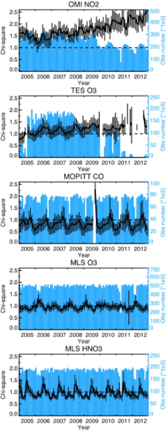
Figure 1 shows the temporal evolution of the number of assimilated observations
(m) andχ2for each assimilated measurement type. The number of super observation
is shown for the OMI NO2 and MOPITT CO. For most cases, the mean values ofχ
2 15
are generally within 50 % difference from the ideal value of 1, which suggests that the
forecast error covariance is reasonably well specified in the data assimilation through-out the reanalysis. Note that the covariance inflation factor for the concentrations and emissions were optimized to approach to the ideal value based on sensitivity
exper-iments (Miyazaki et al., 2012b). For the OMI NO2 assimilation, the χ2 is >1, which
20
indicates overconfidence in the model. Theχ2 for the OMI NO2 was less sensitive to
the choice of the inflation factor compared to that for other assimilated measurements.
ACPD
15, 8687–8770, 2015Tropospheric chemistry reanalysis
K. Miyazaki et al.
Title Page
Abstract Introduction
Conclusions References
Tables Figures
◭ ◮
◭ ◮
Back Close
Full Screen / Esc
Printer-friendly Version Interactive Discussion
Discussion
P
a
per
|
Discussion
P
a
per
|
Discussion
P
a
per
|
Discussion
P
a
per
|
chemical equilibrium states, leading to an underestimation of the background error co-variance during the forecast. Although the emission analysis introduces spread to the concentration ensemble, the perturbations are present primarily near the surface and tend to be removed in the free troposphere because of the short chemical lifetime of
NOx.
5
Overall, theχ2 is constant throughout the reanalysis, which confirms the good
sta-bility of the performance. However, seasonal and interannual variations of theχ2 can
be attributed to variations in the coverage and quality of satellite retrievals as well as changes in atmospheric conditions (e.g., chemical lifetime and dominant transport
type). The increasedχ2 for OMI NO2 after 2010 is associated with a decrease in the
10
number of the assimilated measurements and changes in the super observation er-ror. Both the mean measurement error and the representativeness error (a function of the number of OMI observations) are typically larger in 2010–2012 than in 2005– 2009; the mean measurement error and the total super observation error (a sum of
the measurement error and the representativeness error) averaged over 30–55◦N in
15
January are about 7 and 9 % larger in 2010–2012 than in 2005–2009, respectively.
After 2010, the too largeχ2 indicates underestimations in the analysis spread, while
the increased OmF indicates smaller corrections by the assimilation (cf., Sect. 4.2). To correct the concentrations and emission from OMI super observations that have larger super observation errors, the forecast error needs to be further inflated. A technique to 20
adaptively inflate the forecast error covariance for the concentrations and emissions of
NO and NO2 is required to better represent the data assimilation balance throughout
the reanalysis.
4.2 OmF
OmF statistics are computed in observation space to investigate the structure of 25
model–observation differences and to measure improvements in the reanalysis (Fig. 2).
underes-ACPD
15, 8687–8770, 2015Tropospheric chemistry reanalysis
K. Miyazaki et al.
Title Page
Abstract Introduction
Conclusions References
Tables Figures
◭ ◮
◭ ◮
Back Close
Full Screen / Esc
Printer-friendly Version Interactive Discussion
Discussion
P
a
per
|
Discussion
P
a
per
|
Discussion
P
a
per
|
Discussion
P
a
per
|
timation (i.e., positive OmF) of tropospheric NO2columns compared with the OMI NO2
data from the SH subtropics to NH mid-latitudes, an underestimation of tropospheric CO compared with MOPITT CO data in the NH, an overestimation (i.e., negative OmF)
of middle and upper tropospheric O3in the extratropics compared with TES and MLS
O3 data, and underestimation of middle tropospheric O3 in the tropics compared with
5
TES.
After 2010, the positive OmF for MOPITT CO in the control run decreases in the NH,
and the positive OmF for OMI NO2 increases in the NH mid-latitudes. As the quality
of these retrievals is considered constant in the reanalysis period (e.g., Worden et al., 2013), the interannual variations of OmF are probably attributed to long-term changes 10
in the model bias. The anthropogenic emission inventories for 2008 were used in the model simulation for 2009–2012, which could be partly responsible for the absence of a concentration trend in the model.
In the reanalysis run, the OmF bias and RMSE for MLS O3 becomes nearly zero
globally because of the assimilation. The systematic reductions of the OmF confirm 15
the continuous corrections for model errors by the assimilation. The remaining error is almost equal to the mean observational error. The OmF reduction is relatively smaller
for MLS HNO3than for MLS O3because of the larger observational errors.
The mean OmF bias against TES O3data in the middle troposphere is almost
com-pletely removed because of the assimilation, and the mean OmF RMSE is reduced 20
by about 40 % in the SH extratropics and by up to 15 % from the tropics to the NH. The error reduction is weaker in the lower troposphere (figure not shown) because
of the reduced sensitivity of the TES retrievals to lower tropospheric O3. The analysed
OmF becomes larger after 2010 corresponding to the decreased number of assimilated measurements.
25
con-ACPD
15, 8687–8770, 2015Tropospheric chemistry reanalysis
K. Miyazaki et al.
Title Page
Abstract Introduction
Conclusions References
Tables Figures
◭ ◮
◭ ◮
Back Close
Full Screen / Esc
Printer-friendly Version Interactive Discussion
Discussion
P
a
per
|
Discussion
P
a
per
|
Discussion
P
a
per
|
Discussion
P
a
per
|
stant through the reanalysis, suggesting that the a posteriori emissions realistically represent the interannual variations.
The mean OmF bias against OMI NO2 is reduced with a mean reduction of about
30–60 % at the NH mid-latitudes and about 50–60 % in the tropics. The remaining
errors could be associated with the short chemical lifetime of NOx in the boundary
5
layer as compared to the OMI revisit time of roughly one day, biases in the simulated chemical equilibrium state, and the underestimation of the emission spread. The OmF is relatively larger in 2010–2012 than in other years, corresponding to about half the
reduction in the OMI NO2 observation. The number of assimilated measurements is
important for reducing model errors, even when global coverage is provided. The mean 10
Observation-minus-Analysis (OmA) bias is about 10–15 %; it is smaller in the NH mid-latitudes and almost the same in the tropics and SH compared with the mean OmF in the reanalysis (figure not shown).
4.3 Analysis increment
The analysis increment information, estimated from the differences between the
fore-15
cast and the analysis both in the reanalysis run, is a measure of the adjustment made
in the analysis step. The analysis increment for O3 is mostly positive at 700 hPa and
negative at 400 hPa at mid latitudes (Fig. 3). The positive (negative) increments imply
that the short-term model forecast underestimates (overestimates) the O3
concentra-tions. As the increments are introduced by the TES assimilation, these vertical struc-20
tures suggest that the tropospheric TES O3data have independent information for the
lower and upper tropospheric O3. Assimilation of other measurement generally
pro-vides much smaller increments on the tropospheric O3. The analysis increment varies
largely with season and year, reflecting variations in short-term systematic model er-rors and observational constraints. After 2010 the availability of TES observations is 25
strongly reduced, which explains the small increments in the later years.
The mean analysis increment for NO2varies largely with space and time in the
ACPD
15, 8687–8770, 2015Tropospheric chemistry reanalysis
K. Miyazaki et al.
Title Page
Abstract Introduction
Conclusions References
Tables Figures
◭ ◮
◭ ◮
Back Close
Full Screen / Esc
Printer-friendly Version Interactive Discussion
Discussion
P
a
per
|
Discussion
P
a
per
|
Discussion
P
a
per
|
Discussion
P
a
per
|
mid-latitudes, the NO2 increment becomes negative in the free troposphere because
of the assimilation of non-NO2measurements, compensating for the tropospheric NO2
column changes caused by the (positive) surface emissions adjustment. This demon-strates that simultaneous data assimilation provides independent constraints on the
surface emissions and free tropospheric NO2 concentration, because of the use of
5
observations from multiple species with different measurement sensitivities. Large
ad-justments are introduced to the NO2 concentration in the UTLS, because the MLS O3
and HNO3assimilation effectively corrects the model NO2bias as a result of the
corre-lations between species in the error covariance matrix.
5 Evaluation using independent observations
10
5.1 O3
5.1.1 Ozonesonde
The validation of the reanalysis and control run with global ozonesonde observations is summarised in Table 1. As depicted in Figs. 4 and 5, the CHASER simulation
re-produced the observed main features of global O3distributions in the troposphere and
15
lower stratosphere. However, there are systematic differences such as a negative bias
in the NH high latitude troposphere and a positive bias from the middle troposphere to the lower stratosphere in the SH.
The reanalysis shows improved agreements with the ozonesonde observations. The mean negative bias in the NH high-latitudes is reduced in the troposphere. In the NH 20
mid-latitudes, the model’s positive bias in the UTLS and negative bias in the lower tro-posphere is mostly removed. The large reduction of the mean lower tropospheric bias
in the NH mid-latitudes is attributed primarily to increased O3concentrations in boreal
ACPD
15, 8687–8770, 2015Tropospheric chemistry reanalysis
K. Miyazaki et al.
Title Page
Abstract Introduction
Conclusions References
Tables Figures
◭ ◮
◭ ◮
Back Close
Full Screen / Esc
Printer-friendly Version Interactive Discussion
Discussion
P
a
per
|
Discussion
P
a
per
|
Discussion
P
a
per
|
Discussion
P
a
per
|
surface, are associated with low measurement sensitivities in the lower troposphere and gaps in the spatial representation between the model and observations.
In the tropics, the data assimilation generally increases the O3concentration,
reduc-ing the negative bias in the upper troposphere but increasreduc-ing the positive bias in the lower troposphere. The increased positive bias could be attributed to the positive bias 5
in the TES measurements (Sect. 7.2).
In the SH, the model’s positive bias from the middle troposphere to the lower
strato-sphere is attributed largely to a positive bias in the prescribed O3concentrations above
70 hPa in CHASER, which is mostly removed in the reanalysis. The observed seasonal and interannual variations are captured well in the reanalysis.
10
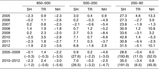
The observed tropospheric O3concentration shows variations from year to year
dur-ing the reanalysis period (Fig. 5). As summarized in Table 2, the reanalysis reveals better agreements with the observed linear slope in most cases. The observed
lin-ear slope during the reanalysis period is positive (+2.9±2.8 ppb (8 years)−1
) at the NH mid-latitudes between 850 and 500 hPa, but the significance of this trend is not very 15
high. The slope over the eight-year period at the same region is also positive in the
reanalysis data (+1.2±2.1 ppb (8 years)−1
), whereas it is negative in the control run
(−1.2±2.1 ppb (8 years)−1). At the NH mid-latitudes in the lower stratosphere (200–
90 hPa), the observed slope is negative (−17.7±41.9 ppb (8 years)−1), whereas the
reanalysis (−25.7±38.8 ppb (8 years)−1) shows better agreement with the observed
20
slope than the control run (−35.8±46.3 ppb (8 years)−1). The seasonal and
year-to-year variations are generally well reproduced in the control run in the NH troposphere
(r=0.73–0.93), whereas the reanalysis further improves the temporal correlation by
0.07 between 850 and 500 hPa and by 0.04 between 500 and 200 hPa at the NH mid-latitudes.
25
The observed time series show obvious year-to-year variations in the tropics
asso-ciated with variations such as in the El Nińo–Southern Oscillation (ENSO), including
their influences on the biomass burning activity. The tropical O3 variations are better
ACPD
15, 8687–8770, 2015Tropospheric chemistry reanalysis
K. Miyazaki et al.
Title Page
Abstract Introduction
Conclusions References
Tables Figures
◭ ◮
◭ ◮
Back Close
Full Screen / Esc
Printer-friendly Version Interactive Discussion
Discussion
P
a
per
|
Discussion
P
a
per
|
Discussion
P
a
per
|
Discussion
P
a
per
|
500 and 200 hPa) than in the control run (r=0.74 andr=0.59). In the tropics and SH,
annual and zonal mean O3concentration does not show clear linear trends during the
reanalysis period either in the observations or reanalysis. However, local O3
concen-trations might have significant trends. For instance, Thompson et al. (2014) showed
wintertime free tropospheric O3increases over Irene and Réunion probably due to that
5
long-range transport of growing pollution in the SH. Further analyses will be required
to investigate the detailed characteristics of O3variation.
The ozonesonde–analysis difference is slightly larger in 2010–2012 than in 2005–
2009 (Table 3 and Fig. 6). The large positive bias throughout the troposphere in win-ter and negative bias below 500 hPa in spring–autumn remain in 2010–2012 (Fig. 6). 10
This is associated with the decreased number of assimilation measurements (TES and OMI); this is discussed further in Sect. 7.3. In contrast, during 2005–2009 the mean
O3 bias does not change significantly with year in the reanalysis, which confirms the
stable performance of the O3reanalysis field. Verstraeten et al. (2013) highlighted that
the time series of the TES-sonde O3biases do not change over time, which suggests
15
that TES is an appropriate instrument for long-term analysis of free tropospheric O3.
5.1.2 Aircraft
Both the model and the reanalysis generally capture well the observed horizontal,
ver-tical, and seasonal variations of O3 concentration compared with the MOZAIC/IAGOS
aircraft measurements (Figs. 7 and 8). However, the model mostly overestimates O3
20
concentration from the northern tropics to the mid-latitudes and underestimates it at the NH high-latitudes in the middle and upper troposphere (between 850 and 300 hPa in Table 1), as consistently revealed by comparison with ozonesonde observations.
An improved agreement with the MOZAIC/IAGOS measurements is found in the re-analysis run, as summarised in Table 1. Most of the negative bias of the model in 25
ACPD
15, 8687–8770, 2015Tropospheric chemistry reanalysis
K. Miyazaki et al.
Title Page
Abstract Introduction
Conclusions References
Tables Figures
◭ ◮
◭ ◮
Back Close
Full Screen / Esc
Printer-friendly Version Interactive Discussion
Discussion
P
a
per
|
Discussion
P
a
per
|
Discussion
P
a
per
|
Discussion
P
a
per
|
the MLS assimilation; the mean positive bias is reduced from+8 % in the control run to
+3 % in the reanalysis. From the NH subtropics to the mid-latitudes, the mean positive
bias of the model at the aircraft–cruising altitude (300–200 hPa) is reduced, whereas the positive bias of low concentration in autumn–winter in the middle troposphere (850– 500 hPa) is increased. In the tropics, the MOZAIC/IAGOS measurements were mostly 5
collected near large biomass–burning areas (Fig. 7: e.g., Central Africa and Southeast
Asia), where O3 concentration in the troposphere becomes too high in the reanalysis
probably attributing to a positive bias in the TES O3observations (cf., Sect. 7.2). Note
that more substantial improvements in comparison with the aircraft measurements are found in 2005–2009 than in the later years.
10
HIPPO measurements provide information on the vertical O3 profiles over the
Pa-cific. The observed tropospheric O3concentration is higher in the extratropics than the
tropics, with higher concentrations in the NH than the SH (Fig. 9). The observed
tropo-spheric O3concentration displays a maximum in the NH subtropics in March (HIPPO3)
because of the strong influence of stratospheric inflows along the westerly jet stream. 15
The observed latitudinal-vertical distributions are generally captured well by both the model and the reanalysis for all the HIPPO campaigns.
The model shows negative biases in the NH extratropics and positive biases from the tropics to the SH compared with the HIPPO measurements (Table 1). These character-istics of the bias are commonly found in comparisons with global ozonesonde observa-20
tions and are reduced effectively in the reanalysis. A considerable bias reduction can be
found in the lower and middle tropospheric O3 at the NH mid-latitudes where O3
vari-ations could be influenced by long-range transport from the Eurasian continent. Direct concentration adjustment by TES measurements in the troposphere and by MLS
mea-surements in the UTLS played important roles in correcting tropospheric O3 profiles.
25
In addition, corrections made to the O3precursors emissions over the Eurasian
conti-nent by OMI, especially over East Asia, were important in influencing tropospheric O3
concentration over the North Pacific around 35–60◦N, especially in boreal spring. This
ACPD
15, 8687–8770, 2015Tropospheric chemistry reanalysis
K. Miyazaki et al.
Title Page
Abstract Introduction
Conclusions References
Tables Figures
◭ ◮
◭ ◮
Back Close
Full Screen / Esc
Printer-friendly Version Interactive Discussion
Discussion
P
a
per
|
Discussion
P
a
per
|
Discussion
P
a
per
|
Discussion
P
a
per
|
by which to correct the global tropospheric O3 profiles, including those over remote
oceans. In contrast, the positive bias in the tropics is further increased in the reanalysis
(from+5 % in the control run to+8 % in the reanalysis between 850 and 500 hPa and
from+10 to+15 % between 500 and 300 hPa), as mostly commonly found in
compar-isons against the MOZAIC/IAGOS and ozonesonde measurements (cf., Sects. 5.1.1 5
and 5.1.2).
Vertical profiles obtained during the NASA aircraft campaigns were also used to
validate the O3 profile (Fig. 10). The comparisons show improved agreements in the
reanalysis in the middle and upper troposphere during INTEX-B over Mexico and dur-ing the ARCTAS campaign over the Arctic. For the DISCOVER-AQ profile, the model’s 10
negative bias in the free troposphere is mostly removed in the reanalysis. For the DC3
profiles, the model captures the observed tropospheric O3 profiles well, whereas the
assimilation leads to small overestimations.
5.2 CO
5.2.1 Surface
15
Surface CO concentrations are compared with the WDCGG surface observations from 59 stations, as summarised in Table 4 and depicted for 12 selected stations in Fig. 11. The control run underestimates CO concentration by up to about 60 ppb in the NH extratropics, with the largest negative bias in winter and smallest bias in summer. The model underestimation has been commonly found in most of the CTMs (Shin-20
dell et al., 2006; Kopacz et al., 2010; Fortems-Cheiney et al., 2011; Stein et al., 2014). The model’s negative bias is also found in most tropical sites, but not in the SH.
Most of the negative bias in the NH extratropics and in the tropics is removed in the reanalysis run, due to the increased surface CO emissions in the analysis (cf., Sect. 6). The MOPITT assimilation dominates the negative bias reduction through the 25
ACPD
15, 8687–8770, 2015Tropospheric chemistry reanalysis
K. Miyazaki et al.
Title Page
Abstract Introduction
Conclusions References
Tables Figures
◭ ◮
◭ ◮
Back Close
Full Screen / Esc
Printer-friendly Version Interactive Discussion
Discussion
P
a
per
|
Discussion
P
a
per
|
Discussion
P
a
per
|
Discussion
P
a
per
|
The annual and regional mean surface bias becomes positive after assimilation at NH mid- and high-latitudes, which is illustrated at locations such as Midway and Bermuda
(32◦N, 65◦W, figure not shown). The observed negative trends at most NH sites are
captured well in the reanalysis.
Tropical CO concentrations show district interannual variations associated with varia-5
tions in tropical biomass-burning activities and meteorological conditions. The temporal correlations with the observations are about 0.1–0.2 higher in the reanalysis compared with the control run in the tropics at Christmas Island and Barbados.
In the SH, the model generally shows good agreement with the surface observations. However, assimilation increases the CO concentration and leads to overestimations in 10
some places (e.g., Showa). The mean negative bias at the SH mid-latitudes changed
from−10 % in the control run to+7 % in the reanalysis.
5.2.2 Aircraft
The model underestimates the CO concentration in the tropics and the NH compared with the MOZAIC/IAGOS aircraft measurements throughout the troposphere (below 15
300 hPa) and around the tropopause at the aircraft–cruising altitude (between 300 and 200 hPa), as depicted in Fig. 12. The model’s negative bias is mostly removed in the reanalysis, with a mean improvement of 50–90 % throughout the troposphere, as sum-marised in Table 4. This confirms that the emission constraints provided at the ground surface are propagated well into the entire troposphere with a delay in the peak tim-20
ing and decay in the amplitude. The spatial distribution in the upper troposphere is also captured well in the reanalysis (Fig. 7). Despite the overall improvement, the low concentrations in the NH lower and middle troposphere in summer and autumn remain underestimated, whereas the analysed concentration becomes too high in the NH high-latitudes at the aircraft-cruising altitude (Fig. 12). A decreasing trend is observed in both 25
ACPD
15, 8687–8770, 2015Tropospheric chemistry reanalysis
K. Miyazaki et al.
Title Page
Abstract Introduction
Conclusions References
Tables Figures
◭ ◮
◭ ◮
Back Close
Full Screen / Esc
Printer-friendly Version Interactive Discussion
Discussion
P
a
per
|
Discussion
P
a
per
|
Discussion
P
a
per
|
Discussion
P
a
per
|
caused unrealistic interannual CO variations and an underestimate of the decreasing trend in the control run.
The distinct interannual variations in the tropics (over Southeast Asia and around Central and North Africa) observed from the MOZAIC/IAGOS aircraft measurements mainly reflect variations in biomass-burning emissions. The temporal variations of CO 5
are captured better by the reanalysis between 850 and 500 hPa (r=0.67 in the control
run and 0.78 in the reanalysis).
The HIPPO observations exhibit large latitudinal CO gradients around 15–25◦N over
the Pacific for all campaigns (Fig. 13). Tropospheric air can be distinguished between the tropics and extratropics because of the transport barrier around the subtropical 10
jet (Bowman, 2002; Miyazaki et al., 2008). The transport barrier produces the large CO gradient in the subtropics and acts to accumulate high levels of CO in the NH extratropics. In the SH, CO concentration increases with height in the free troposphere, because of the strong poleward transport in the upper troposphere from the tropics to the SH high-latitudes.
15
The assimilation increases CO concentration and reduces the mean model nega-tive bias by about 60–80 % in the NH extratropics against the HIPPO measurements. The remaining negative bias could be attributed to overemphasised chemical destruc-tion while air is transported from the Eurasian continent to the HIPPO locadestruc-tions over the central Pacific. For instance, the negative bias of the surface CO concentration is 20
mostly removed in the reanalysis over Yonaguni at the ground surface, located near (downwind of) large sources of Chinese emissions (Fig. 11). This suggests that the emission sources are realistically represented in the reanalysis. Errors in stratospheric CO might also cause the negative bias through stratosphere–troposphere exchange (STE).
25