A tropospheric chemistry reanalysis for the years 2005–2012 based on an assimilation of OMI, MLS, TES, and MOPITT satellite data

(1)

www.atmos-chem-phys.net/15/8315/2015/ doi:10.5194/acp-15-8315-2015

A tropospheric chemistry reanalysis for the years 2005–2012 based

on an assimilation of OMI, MLS, TES, and MOPITT satellite data

K. Miyazaki1, H. J. Eskes2, and K. Sudo3

1_{Japan Agency for Marine-Earth Science and Technology, Yokohama 236-0001, Japan}

2_{Royal Netherlands Meteorological Institute (KNMI), Wilhelminalaan 10, 3732 GK, De Bilt, the Netherlands} 3_{Graduate School of Environmental Studies, Nagoya University, Nagoya, Japan}

Correspondence to:K. Miyazaki (kmiyazaki@jamstec.go.jp)

Received: 19 February 2015 – Published in Atmos. Chem. Phys. Discuss.: 24 March 2015 Revised: 23 June 2015 – Accepted: 9 July 2015 – Published: 27 July 2015

Abstract.We present the results from an 8-year tropospheric chemistry reanalysis for the period 2005–2012 obtained by assimilating multiple data sets from the OMI, MLS, TES, and MOPITT satellite instruments. The reanalysis calcula-tion was conducted using a global chemical transport model and an ensemble Kalman filter technique that simultaneously optimises the chemical concentrations of various species and emissions of several precursors. The optimisation of both the concentration and the emission fields is an efficient method to correct the entire tropospheric profile and its year-to-year variations, and to adjust various tracers chemically linked to the species assimilated. Comparisons against independent aircraft, satellite, and ozonesonde observations demonstrate the quality of the analysed O3, NO2, and CO concentrations on regional and global scales and for both seasonal and year-to-year variations from the lower troposphere to the lower stratosphere. The data assimilation statistics imply persis-tent reduction of model error and improved representation of emission variability, but they also show that discontinuities in the availability of the measurements lead to a degradation of the reanalysis. The decrease in the number of assimilated measurements increased the ozonesonde-minus-analysis dif-ference after 2010 and caused spurious variations in the es-timated emissions. The Northern/Southern Hemisphere OH ratio was modified considerably due to the multiple-species assimilation and became closer to an observational estimate, which played an important role in propagating observational information among various chemical fields and affected the emission estimates. The consistent concentration and emis-sion products provide unique information on year-to-year variations in the atmospheric environment.

1 Introduction

Long-term records of the tropospheric composition of gases such as ozone (O3), carbon monoxide (CO), and nitrogen ox-ides (NOx) are important for understanding the changes in

tropospheric chemistry and human activity and consequences for the atmospheric environment and climate change (HTAP, 2010; IPCC, 2013). Satellite instruments provide observa-tions of the global distribuobserva-tions of tropospheric composition. For example, measurements of tropospheric O3have been re-trieved using the Tropospheric Emission Spectrometer (TES) since 2004 (Beer, 2006) and by the Infrared Atmospheric Sounding Interferometer (IASI) since 2007 (Coman et al., 2012). Tropospheric NO2column concentrations have been retrieved by the Ozone Monitoring Instrument (OMI) since 2004 (Levelt et al., 2006), the Scanning Imaging Absorption Spectrometer for Atmospheric Cartography (SCIAMACHY) from 2002 to 2012 (Bovensmann et al., 1999), the Global Ozone Monitoring Experiment (GOME) from 1996 to 2003, and GOME-2 since 2007 (Callies et al., 2000). The avail-ability of satellite-derived measurements of various chemi-cal species has prompted increasing interest in developing methods for combining these sources of satellite observa-tional information for studies of long-term variations within the atmospheric environment and for improving estimates of emissions sources (Inness et al., 2013; Streets et al., 2013).

Combining measurements of O3, CO and NOx in the

(2)

dif-ferent sources of surface emissions and production of NOx

by lightning (LNOx) (e.g. Martin et al., 2007; Miyazaki et al.,

2014). The information that may be obtained from a com-bined use of multiple satellite data sets without involving a model is limited, related to differing vertical sensitivity pro-files, different overpass times, and mismatches in spatial and temporal coverage between the instruments, as well as miss-ing information on the chemical regime and origin of the air masses.

Data assimilation is the technique for combining different observational data sets with a model by considering the char-acteristics of each measurement (e.g. Kalnay, 2003; Lahoz and Schneider, 2014). Advanced data assimilation schemes like the Kalman filter or the related 4D-Var technique use the information provided by satellite-derived measurements and propagate it, in time and space, from a limited number of observed species to a wide range of chemical components to provide global fields that are physically and chemically consistent and in agreement with the observations. Various studies have demonstrated the capability of data assimilation techniques regarding the analysis of chemical species in the troposphere and stratosphere.

Assimilation of satellite limb measurements for O3 pro-files and nadir measurements for O3columns has been used to study O3variations in the stratosphere and the upper tro-posphere (e.g. Stajner and Wargan, 2004; Jackson, 2007; Sta-jner et al., 2008; Wargan et al., 2010; Flemming et al., 2011; Barré et al., 2013; Emili et al., 2014). Long-term integrated data sets of stratospheric O3 have been produced by sev-eral studies by combining multiple satellite retrieval data sets (e.g. Kiesewetter et al., 2010; van der A et al., 2010). The assimilation of satellite observations has been also applied to investigate global variations in the tropospheric compo-sition of gases such as O3 and CO (e.g. Parrington et al., 2009; Coman et al., 2012; Miyazaki et al., 2012b). For pro-viding long-term integrated data of tropospheric composi-tion, as a pioneer study, Inness et al. (2013) performed an 8-year reanalysis of tropospheric chemistry for 2003–2010 using an advanced data assimilation system. They included atmospheric concentrations of O3, CO, NOx, and

formalde-hyde (CH2O) as the forecast model variables in the integrated forecasting system with modules for atmospheric composi-tion (C-IFS), and they demonstrated improved O3 and CO profiles for the free troposphere. They also highlighted bi-ases remaining in the lower troposphere associated with fixed surface emissions, which are not adjusted in the 4D-Var as-similation scheme presented by Inness et al. (2013).

Currently available bottom-up inventories of emissions, produced based on statistical data such as emission-related activities and emissions factors, contain large uncertainties, mainly because of inaccurate activity rates and emission fac-tors for each category and poor representation of their sea-sonal and interannual variations (e.g. Jaeglé et al., 2005; Xiao et al., 2010; Reuter et al., 2014). Top-down inverse ap-proaches using satellite retrievals have been applied to

ob-tain optimised emissions of CO (e.g. Kopacz et al., 2010; Hooghiemstra et al., 2011) and NOx(e.g. Lamsal et al., 2010;

Miyazaki et al., 2012a; Mijling et al., 2013) by minimising the differences between observed and simulated concentra-tions, as summarised by Streets et al. (2013). In addition to surface emissions, the improved representations of LNOx

sources are important for a realistic representation of O3 formation and chemical processes in the upper troposphere (Schumann and Huntrieser, 2007; Miyazaki et al., 2014).

The simultaneous adjustment of emissions and concen-trations of various species is a new development in tropo-spheric chemical reanalysis and long-term emissions anal-ysis. Miyazaki et al. (2012b) developed a data assimilation system, called CHASER-DAS, for the simultaneous opti-misation of the atmospheric concentration of various trace gases, together with an optimisation of the surface emis-sions of NOx and CO, and the LNOx sources, while taking

their complex chemical interactions into account, as repre-sented by the CHASER chemistry-transport model. Within the simultaneous optimisation framework, the analysis ad-justment of atmospheric concentrations of chemically related species has the potential to improve the emission inversion (Miyazaki and Eskes, 2013; Miyazaki et al., 2014). This was compared with an emission inversion based on mea-surements from one species alone, where uncertainties in the model chemistry affect the quality of the emission source estimates. In addition, the improved estimates of emissions benefit the atmospheric concentration analysis through a re-duction in model forecast error. The simultaneous adjustment of the emissions and the concentrations is therefore a power-ful approach to optimise all aspects of the chemical system influencing tropospheric O3(Miyazaki et al., 2012b).

In this study, we present a tropospheric chemistry re-analysis data set for the 8-year period from 2005 to 2012 using CHASER-DAS. This reanalysis is produced with the CHASER-DAS system introduced in Miyazaki et al. (2012b). The system uses the ensemble Kalman filter (EnKF) assimilation technique and assimilates Microwave Limb Sounder (MLS), OMI, TES, and Measurement of Pol-lution in the Troposphere (MOPITT) retrieved observations. The chemical concentrations and emission sources are simul-taneously optimised during the reanalysis, and are expected to provide useful information for various research topics re-lated to the interannual variability of the atmospheric envi-ronment and short-term trends.

(3)

2 Data assimilation system

The CHASER-DAS system (Miyazaki et al., 2012a, b, 2014; Miyazaki and Eskes, 2013) has been developed based on an EnKF approach and a global chemical transport model called CHASER. The data assimilation settings used for the reanalysis calculation are mostly the same as in Miyazaki et al. (2014), but the calculation was extended to cover the eight years from 2005 to 2012, and several updates were ap-plied to the a priori and state vector settings. Brief descrip-tions of the forecast model, data assimilation approach, and experimental settings are presented below.

2.1 Forecast model

The CHASER model (Sudo et al., 2002; Sudo and Akimoto, 2007) was used as a forecast model. It has so-called T42 horizontal resolution (2.8◦_{for longitude and the T42}

Gaus-sian grid for latitude) and 32 vertical levels from the surface to 4 hPa. It is coupled to the atmospheric general circula-tion model (AGCM) version 5.7b of the Center for Climate System Research and Japanese National Institute for Envi-ronmental Studies (CCSR/NIES). Meteorological fields are provided by the AGCM at every time step of CHASER (i.e. every 20 min). The AGCM fields were nudged toward the National Centers for Environmental Prediction/Department of Energy Atmospheric Model Intercomparison Project II (NCEP-DOE/AMIP-II) reanalysis (Kanamitsu et al., 2002) at every time step of the AGCM to reproduce past meteo-rological fields. The nudged AGCM enabled us to perform CHASER calculations that included short-term atmospheric variations and parameterised transport processes by sub-grid-scale convection and boundary layer mixing.

The a priori value for surface emissions of NOx and CO

were obtained from bottom-up emission inventories. An-thropogenic NOx and CO emissions were obtained from

the Emission Database for Global Atmospheric Research (EDGAR) version 4.2. Emissions from biomass burning are based on the monthly Global Fire Emissions Database (GFED) version 3.1 (van der Werf et al., 2010). Emissions from soils are based on monthly mean Global Emissions In-ventory Activity (GEIA) (Graedel et al., 1993). EDGAR ver-sion 4.2 was not available after 2008 at the time the reanalysis was started; therefore, the emissions for 2008 were used in the calculations for 2009–2012. GFED 3.1 was not available for 2012, and thus the emissions averaged over 2005–2011 were used in the calculation for 2012. For surface NOx

emis-sions, a diurnal variability scheme developed by Miyazaki et al. (2012a, b) was applied depending on the dominant cat-egory for each area: anthropogenic, biogenic, and soil emis-sions.

For the calculation of a priori LNOxemissions, the global

distribution of the flash rate was parameterised in CHASER for convective clouds based on the relation between light-ning activity and cloud top height (Price and Rind, 1992).

To obtain a realistic estimate of the global annual total flash occurrence, a tuning factor was applied for the global total frequency, which is independent of the lightning adjustment in the assimilation. The global distribution of the total flash rate is generally reproduced well by the model in comparison with the observations, except for overestimations over north-ern South America and underestimations over both Central Africa and most of the oceanic Intertropical Convergence Zone (Miyazaki et al., 2014).

2.2 Data assimilation technique

The data assimilation technique employed is an EnKF approach, i.e. a local ensemble transform Kalman filter (LETKF; Hunt et al., 2007) based on the ensemble square root filter (SRF) method, which uses an ensemble forecast to estimate the background error covariance matrix. The covari-ance matrices of the observation error and background error determine the relative weights given to the observation and the background in the analysis. The LETKF has conceptual and computational advantages over the original EnKF. First, the analysis is performed locally in space and time, which re-duces sampling errors caused by limited ensemble size. Sec-ond, performing the analysis independently for different grid points allow parallel computations to be performed that re-duce the computational cost. These advantages are important in the chemical reanalysis calculation because of the many analysis steps included in the 8-year reanalysis run and the large state vector size used for the multiple-states optimisa-tion (cf. Sect. 2.3 and 2.7).

The assimilation step transforms a background ensemble (xb_i_;i₌1, . . ., k) into an analysis ensemble (xa_i_;i₌1, . . ., k) and updates the analysis mean, wherexrepresents the model variable, b the background state, a the analysis state, andk

the ensemble size. The forecast and analysis steps are de-scribed briefly below.

2.2.1 The forecast step

In the forecast step, the background ensemble meanxb_and its perturbationXb are obtained from the evolution of each ensemble member using the forecast model at every model grid,

xb₌1

k k X

i=1

xb_i_; Xb_i ₌xb_i ₋xb_. ₍₁₎

Xb_i is theith column of anN_×kmatrixXb, whereN indi-cates the system dimension (the state vector size times the physical system dimension). Based on the assumption that background ensemble perturbationsXbsample the forecast errors, the background error covariance is estimated as fol-lows:

(4)

where the background error covariancePb varies with time and space, reflecting dominant atmospheric processes and lo-cations of the observations.

An ensemble of background vectorsyb_i and an ensemble of background perturbations in the observation spaceYbare estimated using the observation operatorH (cf. Sect. 2.5):

yb_i ₌Hxb_i_;Yb_i ₌yb_i ₋yb_. ₍₃₎

2.2.2 The analysis step

The analysis ensemble mean is obtained by updating the background ensemble mean:

xa₌_xb₊_Xb_e_Pa₍_Yb₎T_R−1₍_yo

−yb_), ₍₄₎

whereyo represents the observation vector,Ris the p_×p

observation error covariance, andpindicates the number of observations. The observation error information is obtained for each retrieval (cf. Sect. 2.6), whereePais thek_×klocal analysis error covariance in the ensemble space:

e

Pa₌

_(k

−1)I

1₊1 + Y

bT R−1Yb

−1

. (5)

A covariance inflation factor (1₌6 %) was applied to in-flate the forecast error covariance at each analysis step. The inflation is used to prevent an underestimation of background error covariance and resultant filter divergence caused by model errors and sampling errors. The estimation of theePa matrix does not require any calculation of large vectors or matrices withN dimensions in the LETKF algorithm.

The new analysis ensemble perturbation matrix in the model space (Xa) is obtained by transforming the back-ground ensembleXbwithePa:

Xa₌Xb(k₋1)ePa1/2. (6) The new ensemble membersxb_i after the next forecast step are then obtained from model simulations starting from the analysis ensemblexa_i.

2.3 State vector

The state vector for the reanalysis calculation is chosen to op-timise the tropospheric chemical system and to improve the reanalysis performance. The state vector used in the reanal-ysis includes several emission sources (surface emissions of NOx and CO, and LNOx sources) as well as the predicted

concentrations of 35 chemical species. The chemical con-centrations in the state vector are expressed in the form of volume mixing ratio, while the emissions are represented by scaling factors for each surface grid cell for the total NOxand

CO emissions at the surface (not for individual sectors), and for each production rate profile of the LNOx sources.

Per-turbations obtained by adding these model parameters into

the state vector introduced an ensemble spread of chemi-cal concentrations and emissions in the forecast step. The background error correlations, estimated from the ensemble model simulations at each analysis step, determine the rela-tionship between the concentrations and emissions of related species, which can reflect daily, seasonal, interannual, and geographical variations in transport and chemical reactions. The emission sources were optimised at every analysis step throughout the reanalysis period, which reduced the initial bias in the a priori emissions during the data assimilation cy-cle.

2.4 Covariance localisation

The EnKF approach always has the problem of introduc-ing unrealistic long-distance error correlations because of the limited number of ensemble members. During the reanalysis calculation, such spurious correlations lead to errors in the fields that may accumulate and will influence the reanaly-sis quality in a negative way. In order to improve the filter performance, the covariance among non- or weakly related variables in the state vector is set to zero based on sensitivity calculation results, as in Miyazaki et al. (2012b). The anal-ysis of surface emissions of NOx and CO allowed for error

correlations with OMI NO2 and MOPITT CO data, while those with other data were neglected. For the LNOxsources,

covariances with MOPITT CO data were neglected. Concen-trations of NOyspecies and O3were optimised from TES O3, OMI NO2, and MLS O3and HNO3observations. One differ-ence to the study of Miyazaki et al. (2012b) is that concentra-tions of non-methane hydrocarbons (NMHCs) were not op-timised in the reanalysis. The assimilation of MOPITT CO data led to concentrations of NMHCs that increased to unre-alistic values during the reanalysis, likely associated with too much chemical destruction of CO (cf. Sect. 7.4.2).

Covariance localisation was also applied to avoid the influ-ence of remote observations, which is described in Sect. 2.7. 2.5 Observation operator

The observation operator (H) includes the spatial interpola-tion operator (S), a priori profile (xa priori), and averaging ker-nel (A), which maps the model fields (xb_i) into retrieval space (yb_i), thereby accounting for the vertical averaging implicit in the observations, as follows:

yb_i ₌H (xb_i)₌xa priori+A(S(xbi)−xa priori), (7) wherexb_i is the N-dimensional state vector and yb_i is the

(5)

re-trieval a priori profile (Eskes and Boersma, 2003; Migliorini, 2012).

2.6 Observation error

The observation error provided in the retrieval data prod-ucts includes contributions from the smoothing errors, model parameter errors, forward model errors, geophysical noise, and instrument errors. In addition, a representativeness er-ror was added for the OMI NO2and MOPITT CO observa-tions to account for the spatial resolution differences between the model and the observation using a super-observation approach following Miyazaki et al. (2012a). The super-observation error was estimated by considering an error cor-relation of 15 % among the individual satellite observations within a model grid cell.

2.7 Reanalysis settings

Because a single continuous data assimilation calculation for 8 years requires a long computational time, we parallelised the reanalysis calculation. Eight series of 1-year calculations from 1 January of each year in 2005–2012 with a 2-month spin-up starting from 1 November of the previous year were conducted to produce the 8-year reanalysis data set. Each 1-year run was parallelised on 16 processors. The 2-month spin-up removed the differences in the analysis between the different time series, providing a continuous 8-year data set. Because of distinct diurnal variations in the tropospheric chemical system, the data assimilation cycle was set to be short (i.e. 120 min) to reduce sampling errors. The emission and concentration fields were analysed and updated at every analysis step.

In the reanalysis calculation the ensemble size was set to 30, which is somewhat smaller than the 48 members used in our previous studies. A smaller ensemble size reduces com-putational cost but slightly degrades analysis performance, as quantified in Miyazaki et al. (2012b). The horizontal lo-calisation scaleLwas set to 450 km for NOxemissions and

to 600 km for CO emissions, LNOx, and for the

concen-trations. The physical vertical localisation length was set to ln(P1/P2)[hPa]=0.2. These choices are based on sensitiv-ity experiments (Miyazaki et al., 2012b), for which the in-fluence of an observation was set to zero when the horizon-tal distance between the observation and analysis point was larger than 2L_×√10/3 (the cut-off radius is set to 2191 km forL₌600 km). We also account for the influence of the av-eraging kernels of the instruments, which captures the verti-cal sensitivity profiles of the retrievals. The ensemble mem-bers and ensemble spread (error covariance) do vary from one location to the next, and from one species to the next, thereby representing the large number of degrees of freedom contained in the model and the way these are constrained by the observations.

The a priori error was set to 40 % for surface emissions of NOxand CO and 60 % for LNOxsources, but a model error

term was not implemented for emissions during the forecast. To prevent covariance underestimation and maintain emis-sion variability during the long-term reanalysis calculation, we applied covariance inflation to the emission source fac-tors in the analysis step – i.e. model error is implemented through a covariance inflation term. The standard deviation was artificially inflated to a minimum predefined value (30 % of the initial standard deviation) at each analysis step. This was found to be important for representing realistic seasonal and interannual variability in the emission estimates, as con-firmed by the improved agreements between the predicted concentrations and independent observations when this emis-sion covariance inflation setting is used.

In addition to the standard reanalysis run, we conducted a control run for the 8-year period from 2005 to 2012 and several sensitivity calculations for 2005 and 2010 by chang-ing the data assimilation settchang-ings. The control run was per-formed without any data assimilation, but using the same model settings as used in the reanalysis run. The settings and results of sensitivity calculations are presented in Sect. 7.

3 Observations

3.1 Assimilated data sets

The assimilated observations were obtained from the OMI, TES, and MLS on the Aura satellite, launched in July 2004 and from MOPITT on Earth Observing System (EOS) Terra, which was launched in December 1999.

3.1.1 OMI tropospheric NO2column

The OMI provides measurements of both direct and atmosphere-backscattered sunlight in the ultraviolet–visible range (Levelt et al., 2006). The reanalysis used tropo-spheric NO2 column retrievals obtained from the version-2 DOMINO data product (Boersma et al., 2011). The analy-sis increments in the assimilation of OMI NO2were limited to adjust only the surface emissions of NOx, LNOx sources,

and concentrations of NOy species. Low-quality data were

excluded before assimilation following the recommendations of the product’s specification document (Boersma et al., 2011). Since December 2009, approximately half of the pix-els have been compromised by the so-called row anomaly, which reduced the daily coverage of the instrument.

3.1.2 TES O3

(6)

in the tropics and in the summer hemisphere for cloud-free conditions (Worden et al., 2004). The standard quality flags were used to exclude low-quality data (Herman and Kulawik, 2013). We also excluded data poleward of 72◦, because of the small retrieval sensitivity. The data assimilation was per-formed based on the logarithm of the mixing ratio following the retrieval product specification.

3.1.3 MLS O3and HNO3

The MLS data used are the version 3.3 O3and HNO3level 2 products (Livesey et al., 2011). We excluded tropical-cloud-induced outliers, following the recommendations in Livesey et al. (2011). We used data for pressures lower than 215 hPa for O3and 150 hPa for HNO3to constrain the LNOxsources

and concentration of O3and NOyspecies. The accuracy and

precision of the measurement error, described in Livesey et al. (2011), were included as the diagonal element of the observation error covariance matrix.

3.1.4 MOPITT CO

The MOPITT CO data used are the version 6 level 2 TIR products (Deeter et al., 2013). The MOPITT instrument is mainly sensitive to free-tropospheric CO, especially in the middle troposphere, with degrees of freedom for signal (DOFs) typically much larger than 0.5. We excluded data poleward of 65◦and during night-time because of data qual-ity problems (Heald et al., 2004). The data at 700 hPa were used for constraining the surface CO emissions.

3.2 Validation data sets

For the comparisons with satellite observations, the model concentrations were interpolated to the retrieval pixels at the overpass time of the satellite while applying the averaging kernel of each retrieval, and then both the retrieved and sim-ulated concentrations are mapped on a horizontal grid with a resolution of 2.5◦×2.5◦. For comparisons with aircraft and ozonesonde observations, the data were binned on a pressure grid with an interval of 30 hPa and mapped with a horizontal resolution of 5.0◦×5.0◦, while the model output was inter-polated to the time and space of each sample.

3.2.1 GOME-2 and SCIAMACHY NO2

Tropospheric NO2 retrievals were obtained from the TEMIS website (www.temis.nl) and consist of the ver-sion 2.3 GOME-2 and SCIAMACHY products (Boersma et al., 2011). The ground pixel size of the GOME-2 re-trievals is 80 km×40 km with a global coverage within 1.5 days, whereas that of the SCIAMACHY retrievals is 60 km×30 km with global coverage provided approximately once every 6 days. The equatorial overpass times of GOME-2 and SCIAMACHY are at 09:30 and 10:00 LT,

respec-tively. Observations with radiance reflectance of <50 % from clouds with quality flag₌0 were used for validation. 3.2.2 MOZAIC/IAGOS aircraft data

Aircraft O3 and CO measurements obtained from the MOZAIC/IAGOS (Measurement of OZone, water vapour, carbon monoxide and nitrogen oxide by AIrbus in-service airCraft/In-service Aircraft for Global Observing System) programmes (Petzold et al., 2013; Zbinden et al., 2013) were used to validate the tropospheric profiles near airports and the upper-tropospheric spatial distributions at flight altitude of about 12 km in the Northern Hemisphere (NH) and some parts of the tropics. The data are available at www.iagos.fr. The measurements of O3 and CO have an estimated ac-curacy of_±(2 ppb₊2 %) and_±5 ppb (_±5 %), respectively (Zbinden et al., 2013).

3.2.3 HIPPO aircraft data

HIAPER Pole-to-Pole Observation (HIPPO) aircraft mea-surements provide global information on vertical profiles of various species over the Pacific (Wofsy et al., 2012). Latitudinal and vertical variations in O3 and CO obtained from the five HIPPO campaigns (HIPPO I, 8–30 Jan-uary 2009; HIPPO II, 31 October to 22 November 2009; HIPPO III, 24 March to 16 April 2010; HIPPO IV, 14 June to 11 July 2011; and HIPPO V, 9 August to 9 September 2011) were used to validate the assimilated profiles.

3.2.4 NASA aircraft campaign data

Vertical profiles of seven key gases (O3, CO, NO2, OH, HO2, HNO3, and CH2O) obtained from six aircraft cam-paigns – Intercontinental Chemical Transport Experiment Phase B (INTEX-B), Arctic Research of the Composition of the Troposphere from Aircraft and Satellites (ARCTAS)-A, ARCTAS-B, Deriving Information on Surface Conditions from Column and Vertically Resolved Observations Relevant to Air Quality (DISCOVER-AQ), Deep Convection Clouds and Chemistry (DC3)-DC8, and DC3-GV – were used.

The DC-8 measurements obtained during the INTEX-B campaign over the Gulf of Mexico (Singh et al., 2009) were used for the comparison for March 2006. Data collected over highly polluted areas (over Mexico City and Houston) were removed from the comparison, because they can cause seri-ous errors in representativeness (Hains et al., 2010).

The NASA ARCTAS mission (Jacob et al., 2010) was conducted in two 3-week deployments based in Alaska (April 2008, ARCTAS-A) and western Canada (June– July 2008, ARCTAS-B). During ARCTAS-A, most of the measurements were collected between 60 and 90◦N, whereas during ARCTAS-B, the measurements were mainly recorded in the sub-Arctic between 50 and 70◦N.

(7)

extensive profiling of the optical, chemical, and microphysi-cal properties of aerosols (Crumeyrolle et al., 2014).

The Deep Convective Clouds and Chemistry (DC3) ex-periment field campaign investigated the impact of deep, mid-latitude continental convective clouds, including their dynamical, physical, and lightning processes, on upper-tropospheric composition and chemistry during May and June 2012 (Barth et al., 2015). The observations were con-ducted in three locations: northeastern Colorado, western Texas to central Oklahoma, and northern Alabama. The ob-servations obtained from the DC-8 (DC3-DC8) and G-V (DC3-GV) aircraft were used.

3.2.5 Ozonesonde data

Ozonesonde observations taken from the World Ozone and Ultraviolet Radiation Data Center (WOUDC) database (available at http://www.woudc.org) were used to validate the vertical O3profiles. All available data from the WOUDC database are used for the validation (totally 19 273 profiles for 149 stations during 2005–2012). The observation error is 5–10 % between 0 and 30 km (Smit et al., 2007).

3.2.6 WDCGG CO

The CO concentration observations were obtained from the World Data Centre for Greenhouse Gases (WDCGG) op-erated by the World Meteorological Organization (WMO) Global Atmospheric Watch programme (http://ds.data.jma. go.jp/gmd/wdcgg/). Hourly and event observations from 59 stations were used to validate the surface CO concentrations.

4 Data assimilation statistics 4.1 χ2diagnosis

The long-term stability of the data assimilation performance is important in evaluating the reanalysis. Theχ2test can be used to evaluate the data assimilation balance (e.g. Ménard and Chang, 2000), which is estimated from the ratio of the actual observation minus forecast (OmF:yo₋H xb) to the sum of the estimated model and observation error covari-ances in the observational space (HPbHT ₊R), as follows:

Y₌_√1

m(HP

b_HT

+R)−1/2(yo₋H

xb

), (8)

χ2₌traceYYT, (9)

wheremis the number of observations.χ2becomes 1 if the background error covariances (Pb) are properly determined to match with the observed OmF (yo₋H xb) under the presence of the prescribed observation error (R).

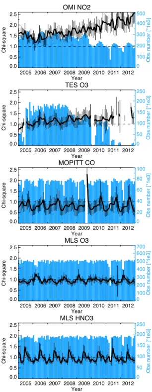
Figure 1 shows the temporal evolution of the number of as-similated observations (m) andχ2for each assimilated mea-surement type. The number of super-observations is shown

for the OMI NO2 and MOPITT CO. For most cases, the mean values ofχ2are generally within 50 % difference from the ideal value of 1, which suggests that the forecast error covariance is reasonably well specified in the data assimila-tion throughout the reanalysis. Note that the covariance in-flation factors for the concentrations and emissions were op-timised to approach to the ideal value based on sensitivity experiments (Miyazaki et al., 2012b). For the OMI NO2 as-similation, theχ2is>1, which indicates overconfidence in the model or underestimation of the super-observation error (computed as a combination of the measurement error and the representativeness error). Theχ2for the OMI NO2was less sensitive to the choice of the inflation factor compared to that for other assimilated measurements. Lower tropospheric NO2is controlled by fast chemical reactions restricted by bi-ased chemical equilibrium states, leading to an underestima-tion of the background error covariance during the forecast. Although the emission analysis introduces spread to the con-centration ensemble, the perturbations are present primarily near the surface and tend to be removed in the free tropo-sphere because of the short chemical lifetime of NOx.

Before 2010, the annual mean χ2 is roughly constant, which confirms the good stability of the performance. Sea-sonal and interannual variations, especially after 2010, inχ2

can be attributed to variations in the coverage and quality of satellite retrievals as well as changes in atmospheric condi-tions (e.g. chemical lifetime and dominant transport type). The increasedχ2for OMI NO2after 2010 is associated with a decrease in the number of the assimilated measurements and changes in the super-observation error. Both the mean measurement error and the representativeness error (a func-tion of the number of OMI observafunc-tions) are typically larger in 2010–2012 than in 2005–2009; the mean measurement er-ror and the total super-observation erer-ror (a sum of the mea-surement error and the representativeness error) averaged over 30–55◦N in January are about 7 and 9 % larger in 2010– 2012 than in 2005–2009, respectively. After 2010, the ex-cessiveχ2indicates underestimations in the analysis spread, while the increased OmF indicates smaller corrections by the assimilation (cf. Sect. 4.2). To correct the concentrations and emission from OMI super-observations that have larger super-observation errors, the forecast error needs to be fur-ther inflated. A technique to adaptively inflate the forecast error covariance for the concentrations and emissions of NO and NO2is required to better represent the data assimilation balance throughout the reanalysis.

4.2 OmF

(8)

MOPITT CO

2005 2006 2007 2008 2009 2010 2011 2012 Year

0.0 0.5 1.0 1.5 2.0 2.5

Chi-square

0 20 40 60 80 100

Obs number [*1e3]

OMI NO2

2005 2006 2007 2008 2009 2010 2011 2012 Year

0.0 0.5 1.0 1.5 2.0 2.5

Chi-square

0 100 200 300 400 500

Obs number [*1e3]

TES O3

2005 2006 2007 2008 2009 2010 2011 2012 Year

0.0 0.5 1.0 1.5 2.0 2.5

Chi-square

0 50 100 150 200 250

Obs number [*1e3]

MLS HNO3

2005 2006 2007 2008 2009 2010 2011 2012 Year

0.0 0.5 1.0 1.5 2.0 2.5

Chi-square

0 50 100 150 200 250

Obs number [*1e3]

MLS O3

2005 2006 2007 2008 2009 2010 2011 2012 Year

0.0 0.5 1.0 1.5 2.0 2.5

Chi-square

0 100 200 300 400 500 600 700

Obs number [*1e3]

Figure 1.Time series of the monthly mean chi-square value and its standard deviation (black lines) and the number of assimilated ob-servations per month (blue bars) for OMI NO2, TES O3, MOPITT CO, MLS O₃, and MLS HNO₃. A super-observation approach is employed to the OMI and MOPITT measurements (the number of super-observations is shown), whereas individual observations are used in the analysis of the others.

positive OmF) of tropospheric NO2columns compared with the OMI NO2data from the Southern Hemisphere (SH) sub-tropics to NH mid-latitudes, an underestimation of tropo-spheric CO compared with MOPITT CO data in the NH, an overestimation (i.e. negative OmF) of middle and upper-tropospheric O3in the extratropics compared with TES and MLS O3 data, and underestimation of middle-tropospheric O3 in the tropics compared with TES. The underestimation of tropospheric CO by CHASER was found to be very sim-ilar to that in most of the other chemistry-transport models (CTMs) (Shindell et al., 2006).

After 2010, the positive OmF for MOPITT CO in the con-trol run decreases in the NH, and the positive OmF for OMI NO2 increases in the NH mid-latitudes. As the quality of these retrievals is considered constant in the reanalysis period (e.g. Worden et al., 2013), the interannual variations in OmF are probably attributed to long-term changes in the model bias. The anthropogenic emission inventories for 2008 were used in the model simulation for 2009–2012, which could be partly responsible for the absence of a concentration trend in the model.

In the reanalysis run, the OmF bias and root-mean-square error (RMSE) for MLS O3becomes nearly zero globally be-cause of the assimilation. The systematic reductions of the OmF confirm the continuous corrections for model errors by the assimilation. The remaining error is almost equal to the mean observational error. The OmF reduction is relatively smaller for MLS HNO3 than for MLS O3 because of the larger observational errors.

The mean OmF bias against TES O3 data in the middle troposphere is almost completely removed because of the as-similation, and the mean OmF RMSE is reduced by about 40 % in the SH extratropics and by up to 15 % from the trop-ics to the NH. The error reduction is weaker in the lower troposphere (figure not shown) because of the reduced sen-sitivity of the TES retrievals to lower-tropospheric O3. The analysed OmF becomes larger after 2010 corresponding to the decreased number of assimilated measurements.

Data assimilation removes most of the OmF bias against MOPITT CO data with a mean bias (RMSE) reduction of about 85 % (60 %) in the NH extratropics and about 80 % (30 %) in the tropics, respectively. The annual mean OmF becomes almost constant through the reanalysis, suggesting that the a posteriori emissions realistically represent the in-terannual variations.

The mean OmF bias against OMI NO2 is reduced with a mean reduction of about 30–60 % at the NH mid-latitudes and about 50–60 % in the tropics. The remaining errors could be associated with the short chemical lifetime of NOx in

(9)

Figure 2.Time–latitude cross section of the monthly and zonal mean OmF obtained without assimilation (left panels) and with assimilation (centre panels). The positive and negative OmF values are shown in red and blue, respectively. Positive OmF represents negative model bias compared with observations. Right panels show latitudinal distributions of the 8-year mean OmF bias (black line) and RMSE (red line) ob-tained with assimilation (solid line) and without assimilation (dotted line). The first row is the OmF for OMI NO2data (in 1015molec cm−2), second row is for TES O3data between 500 and 300 hPa (in ppb), third row is for MOPITT CO data between 700 and 500 hPa (in ppb), fourth row is for MLS O3data between 216 and 100 hPa (in ppm), and fifth row is for MLS HNO3data between 150 and 80 hPa (in ppb). A super-observation approach is employed to the OMI and MOPITT measurements, whereas individual observations are used in the analysis of the others.

is important for reducing model errors, even when global coverage is provided. The mean observation-minus-analysis (OmA) bias is about 10–15 %; it is smaller in the NH mid-latitudes and almost the same in the tropics and SH compared with the mean OmF in the reanalysis (figure not shown). 4.3 Analysis increment

The analysis increment information, estimated from the dif-ferences between the forecast and the analysis both in the

(10)

tropo-2005 2006 2007 2008 2009 2010 2011 2012 -50

0 50

2005 2006 2007 2008 2009 2010 2011 2012 Year

-50 0 50

Latitude

O3 increment at 200 hPa

2005 2006 2007 2008 2009 2010 2011 2012 -50

0 50

-1.0 -0.5 0.0 0.5 1.0

2005 2006 2007 2008 2009 2010 2011 2012 -50

0 50

2005 2006 2007 2008 2009 2010 2011 2012 Year

-50 0 50

Latitude

2005 2006 2007 2008 2009 2010 2011 2012 -50

0 50

-0.10 -0.05 0.00 0.05 0.10 2005 2006 2007 2008 2009 2010 2011 2012

-50 0 50

2005 2006 2007 2008 2009 2010 2011 2012 Year

-50 0 50

Latitude

2005 2006 2007 2008 2009 2010 2011 2012 -50

0 50

-0.10 -0.05 0.00 0.05 0.10

2005 2006 2007 2008 2009 2010 2011 2012 -50

0 50

2005 2006 2007 2008 2009 2010 2011 2012 Year

-50 0 50

Latitude

O3 spread at 200 hPa

2005 2006 2007 2008 2009 2010 2011 2012 -50

0 50

0 500 1000 1500 2000 2500 3000 2005 2006 2007 2008 2009 2010 2011 2012

-50 0 50

2005 2006 2007 2008 2009 2010 2011 2012 Year

-50 0 50

Latitude

2005 2006 2007 2008 2009 2010 2011 2012 -50

0 50

0 5 10 15 20

2005 2006 2007 2008 2009 2010 2011 2012 -50

0 50

2005 2006 2007 2008 2009 2010 2011 2012 Year

-50 0 50

Latitude

2005 2006 2007 2008 2009 2010 2011 2012 -50

0 50

0 5 10 15 20

Figure 3.Time–latitude cross section of the analysis increment (upper panels, in ppb per analysis step) and the analysis spread (lower panels, in ppb/analysis step) obtained for O3at 700 hPa (left), 400 hPa (centre), and 200 hPa (right).

sphere, with the largest DOFs for clear-sky scenes occurring at low latitudes where TES can distinguish between lower-and upper-tropospheric O3. The obtained analysis increments correspond well to the OmF in the control run at the same altitude (figure not shown), confirming that the data assimi-lation effectively reduced the model errors through the anal-ysis steps. Assimilation of other measurement generally pro-vides much smaller increments on the tropospheric O3. The analysis increment varies largely with season and year, re-flecting variations in short-term systematic model errors and observational constraints. After 2010 the availability of TES observations is strongly reduced, which explains the small increments in the later years.

The mean analysis increment for NO2varies largely with space and time in the troposphere (not shown). For some re-gions with strong surface emissions, especially at NH mid-latitudes, the NO2 increment becomes negative in the free troposphere because of the assimilation of non-NO2 mea-surements, compensating for the tropospheric NO2column changes caused by the (positive) surface emissions adjust-ment. This demonstrates that simultaneous data assimilation provides independent constraints on the surface emissions and free-tropospheric NO2concentration, because of the use of observations from multiple species with different mea-surement sensitivities. Large adjustments are introduced to the NO2concentration in the upper troposphere–lower strato-sphere (UTLS), because the MLS O3and HNO3assimilation effectively corrects the model NO2bias as a result of the cor-relations between species in the error covariance matrix.

5 Evaluation using independent observations 5.1 O3

5.1.1 Ozonesonde

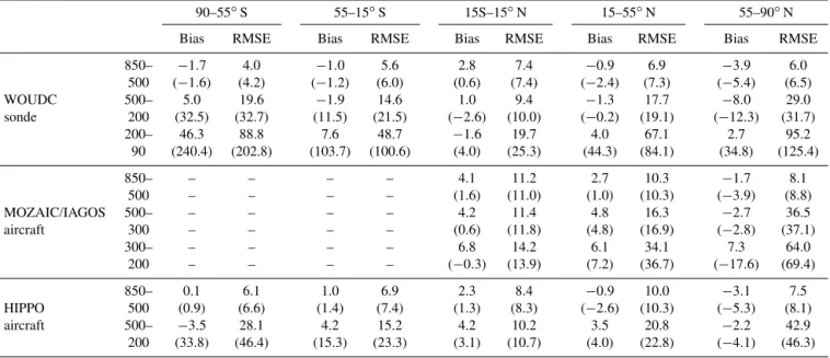
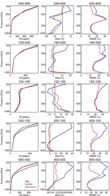
The validation of the reanalysis and control run with global ozonesonde observations is summarised in Table 1. As de-picted in Figs. 4 and 5, the CHASER simulation reproduced the observed main features of global O3distributions in the troposphere and lower stratosphere. However, there are sys-tematic differences such as a negative bias in the NH high-latitude troposphere and a positive bias from the middle tro-posphere to the lower stratosphere in the SH.

The reanalysis shows improved agreements with the ozonesonde observations. The mean negative bias in the NH high latitudes is reduced in the troposphere. In the NH mid-latitudes, the model’s positive bias in the UTLS and nega-tive bias in the lower troposphere is mostly removed. The large reduction of the mean lower-tropospheric bias in the NH mid-latitudes is attributed primarily to increased O3 con-centrations in boreal spring–summer (Fig. 5). The RMSEs compared with the ozonesonde observations are also reduced throughout the troposphere. The remaining errors, especially near the surface, are associated with low retrieval sensitivities in the lower troposphere and gaps in the spatial representa-tion between the model and observarepresenta-tions.

In the tropics, the data assimilation generally increases the O3concentration, reducing the negative bias in the upper tro-posphere but increasing the positive bias in the lower tropo-sphere. The increased positive bias could be attributed to the positive bias in the TES measurements (Sect. 7.2).

(11)

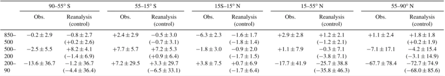
posi-Table 1.Model minus observation comparisons of the mean O3concentrations between the analysis or control run (in brackets) and the observations. The units of the root-mean-square error (RMSE) and bias are ppb. Results are provided for WOUDC ozonesonde observations during 2005–2012, MOZAIC/IAGOS aircraft measurements during 2005–2012, and HIPPO aircraft measurements during 2009–2011.

90–55◦S 55–15◦S 15S–15◦N 15–55◦N 55–90◦N

Bias RMSE Bias RMSE Bias RMSE Bias RMSE Bias RMSE

850– ₋1.7 4.0 ₋1.0 5.6 2.8 7.4 ₋0.9 6.9 ₋3.9 6.0

500 (−1.6) (4.2) (−1.2) (6.0) (0.6) (7.4) (−2.4) (7.3) (−5.4) (6.5)

WOUDC 500– 5.0 19.6 −1.9 14.6 1.0 9.4 −1.3 17.7 −8.0 29.0

sonde 200 (32.5) (32.7) (11.5) (21.5) (−2.6) (10.0) (−0.2) (19.1) (−12.3) (31.7)

200– 46.3 88.8 7.6 48.7 ₋1.6 19.7 4.0 67.1 2.7 95.2

90 (240.4) (202.8) (103.7) (100.6) (4.0) (25.3) (44.3) (84.1) (34.8) (125.4)

850– – – – – 4.1 11.2 2.7 10.3 ₋1.7 8.1

500 – – – – (1.6) (11.0) (1.0) (10.3) (−3.9) (8.8)

MOZAIC/IAGOS 500– – – – – 4.2 11.4 4.8 16.3 −2.7 36.5

aircraft 300 – – – – (0.6) (11.8) (4.8) (16.9) (₋2.8) (37.1)

300– – – – – 6.8 14.2 6.1 34.1 7.3 64.0

200 – – – – (−0.3) (13.9) (7.2) (36.7) (−17.6) (69.4)

850– 0.1 6.1 1.0 6.9 2.3 8.4 −0.9 10.0 −3.1 7.5

HIPPO 500 (0.9) (6.6) (1.4) (7.4) (1.3) (8.3) (−2.6) (10.3) (−5.3) (8.1)

aircraft 500– ₋3.5 28.1 4.2 15.2 4.2 10.2 3.5 20.8 ₋2.2 42.9

200 (33.8) (46.4) (15.3) (23.3) (3.1) (10.7) (4.0) (22.8) (−4.1) (46.3)

tive bias in the prescribed O3concentrations above 70 hPa in CHASER, which is mostly removed in the reanalysis. The observed seasonal and interannual variations are captured well in the reanalysis.

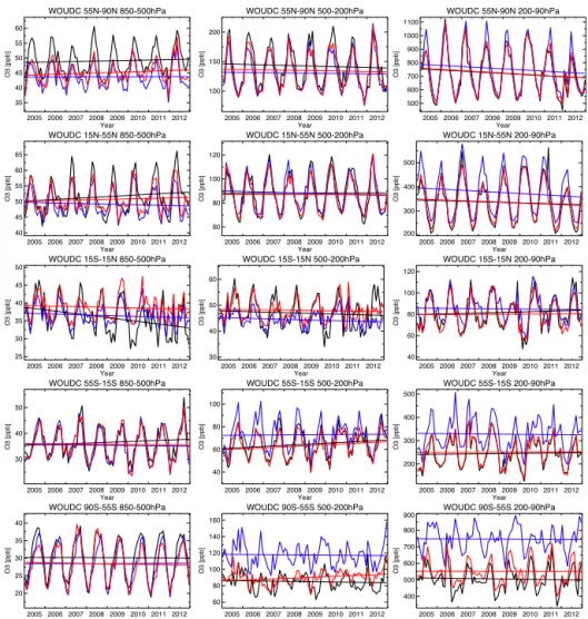
The observed tropospheric O3concentration shows varia-tions from year to year during the reanalysis period (Fig. 5). As summarised in Table 2, the reanalysis reveals better agree-ments with the observed linear slope in most cases. The observed linear slope during the reanalysis period is posi-tive (+2.9±2.8 ppb(8 years)−1) at the NH mid-latitudes be-tween 850 and 500 hPa, but the significance of this trend is not very high. The slope over the 8-year period at the same region is also positive in the reanalysis data (+1.2±

2.1 ppb(8 years)−1), whereas it is negative in the control run (−1.2±2.1 ppb(8 years)−1). At the NH mid-latitudes in the lower stratosphere (200–90 hPa), the observed slope is negative (−17.7±41.9 ppb(8 years)−1), whereas the re-analysis (−25.7±38.8 ppb(8 years)−1) shows better agree-ment with the observed slope than the control run (−35.8±

46.3 ppb(8 years)−1). The seasonal and year-to-year varia-tions are generally well reproduced in the control run in the NH troposphere (r₌0.73–0.93), whereas the reanalysis fur-ther improves the temporal correlation by 0.07 between 850 and 500 hPa and by 0.04 between 500 and 200 hPa at the NH mid-latitudes.

The observed time series show obvious year-to-year vari-ations in the tropics associated with varivari-ations such as in the El Niño–Southern Oscillation (ENSO), including their influences on the biomass-burning activity. The tropical O3 variations are better represented in the reanalysis (r₌0.80 between 850 and 500 hPa and r₌0.72 between 500 and

200 hPa) than in the control run (r₌0.74 andr₌0.59). In the tropics and SH, annual and zonal mean O3concentration does not show clear linear trends during the reanalysis period either in the observations or reanalysis. However, local O3 concentrations might have significant trends. For instance, Thompson et al. (2014) showed wintertime free-tropospheric O3 increases over Irene and Réunion probably due to long-range transport of growing pollution in the SH. Further anal-yses will be required to investigate the detailed characteris-tics of O3variation.

The ozonesonde–analysis difference is slightly larger in 2010–2012 than in 2005–2009 (Table 3 and Fig. 6). The large positive bias throughout the troposphere in winter and neg-ative bias below 500 hPa in spring–autumn remain in 2010– 2012 (Fig. 6). This is associated with the decreased number of assimilation measurements (TES and OMI); this is dis-cussed further in Sect. 7.3. In contrast, during 2005–2009 the mean O3bias does not change significantly with year in the reanalysis, which confirms the stable performance of the O3 reanalysis field. Verstraeten et al. (2013) highlighted that the time series of the TES–sonde O3biases do not change over time, which suggests that TES is an appropriate instrument for long-term analysis of free-tropospheric O3.

5.1.2 Aircraft

(12)

lati-90S-55S

-20-10 0 102030405060 Bias [%] 100 200 500 1000 90S-55S

0 300 600

O3 [ppbv] 100 200 500 1000 Pressure [hPa] 90S-55S

0 10 20 30 40 50 RMSE [%] 100 200 500 1000 55S-15S

0 10 20 30 40 Bias [%] 100 200 500 1000 55S-15S 0 300 O3 [ppbv] 100 200 500 1000 Pressure [hPa] 55S-15S

0 10 20 30 40 RMSE [%] 100 200 500 1000 15S-15N

-10 0 10 20 30 Bias [%] 100 200 500 1000 15S-15N 0 O3 [ppbv] 100 200 500 1000 Pressure [hPa] 15S-15N

0 10 20 30

RMSE [%] 100 200 500 1000 15N-55N

0 10 20

Bias [%] 100 200 500 1000 15N-55N 0 300 O3 [ppbv] 100 200 500 1000 Pressure [hPa] 15N-55N

0 10 20 30

RMSE [%] 100 200 500 1000 55N-90N

-20 -10 0 10

Bias [%] 100 200 500 1000 55N-90N

0 300 600 900 O3 [ppbv] 100 200 500 1000 Pressure [hPa] 55N-90N

0 10 20 30

RMSE [%] 100 200 500 1000 Obs Control Reanalysis

Figure 4.Comparison of the vertical O3profiles between ozoneson-des (black), control run (blue), and reanalysis (red) averaged for the period 2005–2012. The left column shows the mean profile; centre and right columns show the mean difference and the RMSE between the control run and the observations (blue) and between the reanaly-sis and the observations (red). From top to bottom, results are shown for the NH high latitudes (55–90◦N), NH mid-latitudes (15–55◦N), tropics (15◦S–15◦N), SH mid-latitudes (15–55◦S), and SH high latitudes (55–90◦S).

tudes in the middle and upper troposphere (between 850 and 300 hPa in Table 1), as consistently revealed by comparison with ozonesonde observations.

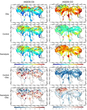
Although the improvement is not large in the upper tropo-sphere (500–300 hPa, Fig. 7), an improved agreement with the MOZAIC/IAGOS measurements is found in the reanaly-sis run in the middle troposphere (850–500 hPa) and at the aircraft cruising altitude (300–200 hPa), as summarised in

Table 1. Most of the negative bias of the model in the tro-posphere of the NH high latitudes is reduced throughout the reanalysis period. A substantial improvement is observed at the aircraft cruising altitude around the tropopause (between 300 and 200 hPa) at the NH high latitudes; the mean positive bias is reduced from+8 % in the control run to+3 % in the reanalysis. By separately assimilating individual measure-ments through the observing system experimeasure-ments (OSEs), we confirmed that the improvement is mainly attributed to the MLS assimilation (not shown).

From the NH subtropics to the mid-latitudes, the mean positive bias of the model at the aircraft cruising alti-tude (300–200 hPa) is reduced, whereas the positive bias of low concentration in autumn–winter in the middle tro-posphere (850–500 hPa) is increased. In the tropics, the MOZAIC/IAGOS measurements were mostly collected near large biomass-burning areas (Fig. 7: e.g. Central Africa and Southeast Asia), where O3concentration in the troposphere becomes too high in the reanalysis probably attributed to a positive bias in the TES O3 observations (cf. Sect. 7.2). Note that more substantial improvements in comparison with the aircraft measurements are found in 2005–2009 than in the later years.

HIPPO measurements provide information on the vertical O3 profiles over the Pacific. The observed tropospheric O3 concentration is higher in the extratropics than the tropics, with higher concentrations in the NH than the SH (Fig. 9). The observed tropospheric O3concentration displays a maxi-mum in the NH subtropics in March (HIPPO3) because of the strong influence of stratospheric inflows along the westerly jet stream. The observed latitudinal–vertical distributions are generally captured well by both the model and the reanalysis for all the HIPPO campaigns.

The model shows negative biases in the NH extratropics and positive biases from the tropics to the SH compared with the HIPPO measurements (Table 1). These characteristics of the bias are commonly found in comparisons with global ozonesonde observations in this study (cf. Sect. 5.1.1) and are reduced effectively in the reanalysis. A considerable bias reduction can be found in the lower- and middle-tropospheric O3 at the NH mid-latitudes where O3 variations could be influenced by long-range transport from the Eurasian con-tinent. Direct concentration adjustment by TES measure-ments in the troposphere and by MLS measuremeasure-ments in the UTLS played important roles in correcting tropospheric O3 profiles. In addition, corrections made to the O3 precursors emissions over the Eurasian continent by OMI, especially over East Asia, were important in influencing tropospheric O3 concentration over the North Pacific around 35–60◦N, especially in boreal spring. This demonstrates that the as-similation of multiple-species data sets is a powerful means by which to correct the global tropospheric O3profiles, in-cluding those over remote oceans. In contrast, the positive bias in the tropics is further increased in the reanalysis (from

(13)

WOUDC 15S-15N 850-500hPa

2005 2006 2007 2008 2009 2010 2011 2012 Year

25 30 35 40 45 50

O3 [ppb]

2005 2006 2007 2008 2009 2010 2011 2012 Year

30 40 50 60

O3 [ppb]

2005 2006 2007 2008 2009 2010 2011 2012 Year

40 60 80 100 120

O3 [ppb]

WOUDC 55S-15S 850-500hPa

2005 2006 2007 2008 2009 2010 2011 2012 Year

30 40 50

O3 [ppb]

2005 2006 2007 2008 2009 2010 2011 2012 Year

40 60 80 100

O3 [ppb]

2005 2006 2007 2008 2009 2010 2011 2012 Year

200 300 400 500

O3 [ppb]

2005 2006 2007 2008 2009 2010 2011 2012 Year

20 25 30 35 40

O3 [ppb]

2005 2006 2007 2008 2009 2010 2011 2012 Year

60 80 100 120 140 160

O3 [ppb]

2005 2006 2007 2008 2009 2010 2011 2012 Year

400 500 600 700 800 900

O3 [ppb]

WOUDC 55N-90N 850-500hPa

2005 2006 2007 2008 2009 2010 2011 2012 Year

35 40 45 50 55 60

O3 [ppb]

2005 2006 2007 2008 2009 2010 2011 2012 Year

100 150 200

O3 [ppb]

2005 2006 2007 2008 2009 2010 2011 2012 Year

500 600 700 800 900 1000 1100

O3 [ppb]

2005 2006 2007 2008 2009 2010 2011 2012 Year

40 45 50 55 60 65

O3 [ppb]

2005 2006 2007 2008 2009 2010 2011 2012 Year

60 80 100 120

O3 [ppb]

2005 2006 2007 2008 2009 2010 2011 2012 Year

200 300 400 500

O3 [ppb]

Figure 5.Time series of the monthly mean O₃concentration obtained from ozonesondes (black), control run (blue), and reanalysis (red) averaged between 850 and 500 hPa (left column), 500 and 200 hPa (centre column), and 200 and 90 hPa (right column). From top to bottom the results are shown for the NH high latitudes (55–90◦N), NH mid-latitudes (15–55◦N), tropics (15◦S–15◦N), SH mid-latitudes (15– 55◦S), and SH high latitudes (55–90◦S).

850 and 500 hPa and from₊10 to₊15 % between 500 and 300 hPa), as mostly commonly found in comparisons against the MOZAIC/IAGOS and ozonesonde measurements (cf. Sect. 5.1.1 and 5.1.2).

Vertical profiles obtained during the NASA aircraft cam-paigns were also used to validate the O3 profile (Fig. 10). The comparisons show improved agreements in the reanal-ysis in the middle and upper troposphere during INTEX-B over Mexico and during the ARCTAS campaign over the Arctic, but the model’s positive bias near the surface is fur-ther increased for the INTEX-B profile. For the DISCOVER-AQ profile, the model’s negative bias in the free troposphere is mostly removed in the reanalysis. For the DC3 profiles, the model captures the observed tropospheric O3profiles well, whereas the assimilation leads to small overestimations.

5.2 CO 5.2.1 Surface

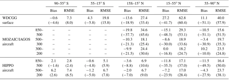
Surface CO concentrations are compared with the WDCGG surface observations from 59 stations, as summarised in Ta-ble 4 and depicted for 12 selected stations in Fig. 11. The control run underestimates CO concentration by up to about 60 ppb in the NH extratropics, with the largest negative bias in winter and smallest bias in summer. The model under-estimation has been commonly found in most of the CTMs (Shindell et al., 2006; Kopacz et al., 2010; Fortems-Cheiney et al., 2011; Stein et al., 2014). The model’s negative bias is also found in most tropical sites, but not in the SH.

(14)

Table 2.Linear trend (slope in ppb(8 years)−1) and standard deviation (in ppb) of O3derived from the WMO ozonesonde observations, the control run, and the reanalysis during 2005–2012.

90–55◦S 55–15◦S 15S–15◦N 15–55◦N 55–90◦N

Obs. Reanalysis Obs. Reanalysis Obs. Reanalysis Obs. Reanalysis Obs. Reanalysis

(control) (control) (control) (control) (control)

850– −0.2±2.9 −0.8±2.7 +2.4±2.9 −0.5±3.0 −6.3±2.3 −1.6±1.7 +2.9±2.8 +1.2±2.1 +1.1±2.4 +1.8±1.8 500 (+0.2±2.6) (−0.7±3.1) (−1.8±1.4) (−1.2±2.1) (+0.2±1.9) 500– −2.5±5.5 +8.2±4.1 +7.7±5.7 +7.2±5.3 −1.8±3.0 −0.9±2.0 +1.1±7.9 −0.3±7.1 −7.1±17.1 −4.2±15.4 200 (−1.4±6.9) (+0.9±6.4) (−1.7±1.5) (−3.8±7.1) (−3.1±14.9) 200– −13.6±36.7 −1.2±36.7 +7.2±29.5 +3.3±29.7 +3.8±7.5 +0.7±6.9 −17.7±41.9 −25.7±38.8 −67.7±78.4 −72.7±74.9 90 (−4.4±36.4) (−6.5±33.1) (−1.7±6.4) (−35.8±46.3) (−68.0±85.6)

Table 3.Comparisons of the mean O3concentrations between the reanalysis run and the WOUDC ozonesonde observations in the Southern Hemisphere (SH) (90–30◦S), troposphere (TR) (30◦S–30◦N) and Northern Hemisphere (NH) (30–90◦N). The mean differences are shown for each year of the reanalysis period and for mean concentrations during 2005–2009 and during 2010–2012. The latter includes results for the control run given in brackets.

850–500 hPa 500–200 hPa 200–90 hPa

SH TR NH SH TR NH SH TR NH

2005 −2.3 0.9 −2.3 3.0 0.4 0.9 27.3 4.6 13.3

2006 −0.2 1.1 −2.6 0.2 −0.3 −4.9 27.3 −2.7 3.9

2007 0.2 0.8 ₋2.5 ₋2.1 ₋0.6 ₋5.4 23.8 ₋1.9 ₋1.3

2008 1.4 1.9 −1.8 0.7 1.2 −5.2 30.9 1.2 10.8

2009 0.2 2.3 ₋2.0 2.7 0.3 ₋8.4 33.6 ₋3.1 3.2

2010 −2.5 3.5 −2.8 7.1 0.7 −6.6 42.8 1.4 −5.3

2011 −2.3 1.8 −2.7 7.1 0.3 −3.7 30.8 −6.4 −2.5

2012 −1.9 2.0 −3.6 6.8 −1.6 2.9 31.5 −5.1 10.1

2005–2009 −0.1 1.4 −2.2 0.9 0.2 −4.6 28.6 −0.4 6.0

(−0.3) (−0.3) (−3.5) (27.6) (−2.2) (−3.0) (193.8) (11.0) (52.0)

2010–2012 −2.3 2.4 −3.0 7.0 −0.2 −2.5 35.0 −3.4 0.8

(₋1.2) (₋0.6) (₋5.6) (26.5) (₋3.2) (₋4.7) (191.0) (6.5) (45.9)

through the surface CO emission optimisation, whereas the assimilation of other data has only a small influence on the CO concentration analysis through changes in the OH field. The annual and regional mean surface bias becomes positive after assimilation at NH mid- and high latitudes, which is il-lustrated at locations such as Midway and Bermuda (32◦N, 65◦W; figure not shown). The observed negative trends at most NH sites are captured well in the reanalysis.

Tropical CO concentrations show district interannual vari-ations associated with varivari-ations in tropical biomass-burning activities and meteorological conditions. The temporal cor-relations with the observations are about 0.1–0.2 higher in the reanalysis compared with the control run in the tropics at Christmas Island and Barbados.

In the SH, the model generally shows good agreement with the surface observations. However, assimilation increases the CO concentration and leads to overestimations in some places (e.g. Showa). The mean negative bias at the SH mid-latitudes changed from−10 % in the control run to+7 % in the reanalysis.

5.2.2 Aircraft

(15)

2005 2006 2007 2008 2009 2010 2011 2012 1000

500 200

2005 2006 2007 2008 2009 2010 2011 2012 Year

1000 500 200

Pressure

Reanalysis - Obs [%]

2005 2006 2007 2008 2009 2010 2011 2012 1000

500 200

-20 -10 0 10 20

2005 2006 2007 2008 2009 2010 2011 2012 1000

500 200

2005 2006 2007 2008 2009 2010 2011 2012 Year

1000 500 200

Pressure

Control - Obs [%]

2005 2006 2007 2008 2009 2010 2011 2012 1000

500 200

Figure 6.Vertical profiles of the time series of the monthly mean O3 concentration difference (in %) between the control run and ozonesondes (top) and between the reanalysis and ozonesondes (bottom) averaged over the NH mid-latitudes (15–55◦N).

represented realistically in the reanalysis. The EDGAR 4.2 for 2008 was used for the model simulation for 2009–2012. The analysis and the comparison with the independent ob-servations show that this caused unrealistic interannual CO variations and an underestimate of the decreasing trend in the control run.

The distinct interannual variations in the tropics (over Southeast Asia and around Central and North Africa) ob-served from the MOZAIC/IAGOS aircraft measurements mainly reflect variations in biomass-burning emissions. The temporal variations of CO are captured better by the reanaly-sis between 850 and 500 hPa (r₌0.67 in the control run and 0.78 in the reanalysis).

The HIPPO observations exhibit large latitudinal CO gra-dients around 15–25◦N over the Pacific for all campaigns (Fig. 13). Tropospheric air can be distinguished between the tropics and extratropics because of the transport bar-rier around the subtropical jet (Bowman and Carrie, 2002; Miyazaki et al., 2008). The transport barrier produces the large CO gradient in the subtropics and acts to accumulate high levels of CO in the NH extratropics. In the SH, CO concentration increases with height in the free troposphere, because of the strong poleward transport in the upper tropo-sphere from the tropics to the SH high latitudes.

Figure 7.Spatial distributions of O3(left column) and CO (right column) averaged between 500 and 300 hPa and during 2005–2012 obtained from the MOZAIC/IAGOS aircraft measurements (first row), control run (second row), and reanalysis (third row). Differ-ences between the control run and observations (fourth row) and between the reanalysis and observations (fifth row) are also plotted. Units are ppb.

The assimilation increases CO concentration and reduces the mean model negative bias by about 60–80 % in the NH extratropics against the HIPPO measurements. The re-maining negative bias could be attributed to overempha-sised chemical destruction while air is transported from the Eurasian continent to the HIPPO locations over the central Pacific. For instance, the negative bias of the surface CO concentration is mostly removed in the reanalysis over Yona-guni at the ground surface, located near (downwind of) large sources of Chinese emissions (Fig. 11). This suggests that the emission sources are realistically represented in the reanaly-sis. Errors in stratospheric CO might also cause the negative bias through stratosphere–troposphere exchange (STE).

(16)

repre-Table 4.Same as Table 1, but for mean CO concentrations. Units are ppb. Observations used are the WDCGG observations during 2005– 2012, MOZAIC/IAGOS aircraft measurements during 2005–2012, and HIPPO aircraft measurements during 2009–2011.

90–55◦S 55–15◦S 15S–15◦N 15–55◦N 55–90◦N

Bias RMSE Bias RMSE Bias RMSE Bias RMSE Bias RMSE

WDCGG −0.6 7.3 4.3 19.8 −13.6 27.4 27.2 62.8 11.1 40.0

surface (−4.6) (8.0) (−5.8) (15.8) (−18.9) (33.4) (−41.7) (60.4) (−51.1) (57.9)

850– – – – – −19.8 34.6 −15.1 29.3 −10.5 15.6

500 – – – – (−37.7) (45.6) (−48.3) (53.1) (−51.1) (51.5)

MOZAIC/IAGOS 500– – – – – ₋10.3 18.1 ₋8.6 18.9 ₋3.4 19.7

aircraft 300 – – – – (−21.3) (25.4) (−30.0) (33.6) (−30.9) (35.3)

300– – – – – −9.9 24.4 0.0 18.2 10.2 23.5

200 – – – – (₋21.5) (30.6) (₋16.8) (24.7) (₋10.0) (24.8)

850– 2.1 2.8 −0.6 5.1 −3.6 6.9 −11.8 17.1 −11.5 16.4

HIPPO 500 (₋1.6) (2.4) (₋4.8) (5.9) (₋8.8) (10.6) (₋35.3) (37.0) (₋49.5) (50.0)

aircraft 500– 6.2 7.4 −1.2 6.7 −2.0 6.7 −7.2 17.0 −4.3 23.7

200 (2.6) (6.5) (−5.0) (7.8) (−7.0) (9.0) (−23.9) (28.4) (−27.9) (38.1)

IAGOS 50N-90N 500-300hPa

2005 2006 2007 2008 2009 2010 2011 2012 Year

50 100 150 200

O3 [ppb]

2005 2006 2007 2008 2009 2010 2011 2012 Year

100 150 200 250 300 350 400

O3 [ppb]

2005 2006 2007 2008 2009 2010 2011 2012 Year

60 80 100 120

O3 [ppb]

2005 2006 2007 2008 2009 2010 2011 2012 Year

100 150 200

O3 [ppb]

IAGOS 15S-15N 500-300hPa

2005 2006 2007 2008 2009 2010 2011 2012 Year

40 50 60 70 80

O3 [ppb]

2005 2006 2007 2008 2009 2010 2011 2012 Year

30 40 50 60 70 80

O3 [ppb]

2005 2006 2007 2008 2009 2010 2011 2012 Year

35 40 45 50 55 60 65

O3 [ppb]

2005 2006 2007 2008 2009 2010 2011 2012 Year

20 30 40 50 60 70

O3 [ppb]

2005 2006 2007 2008 2009 2010 2011 2012 Year

40 50 60 70

O3 [ppb]

Figure 8.Time series of the monthly mean O3concentration obtained from the MOZAIC/IAGOS aircraft measurements (black), control run (blue), and reanalysis (red) averaged between 850 and 500 hPa (left column), 500 and 300 hPa (centre column), and 300 and 200 hPa (right column). From top to bottom the results are shown for the NH high latitudes (55–90◦N), NH mid-latitudes (15–55◦N), and tropics (15◦S–15◦N).

sents the Asian anthropogenic emissions and their influences on the western Arctic CO level. Bian et al. (2013) also sug-gested a lower fraction of CO from Asian anthropogenic emissions during the B than during the ARCTAS-A and showed that the along-track measurements are not rep-resentative of the concentrations within the large domain of the western Arctic during the ARCTAS-B, which may ex-plain the small bias reduction for the ARCTAS-B profile in

our comparison. MOPITT data are assimilated equatorward of 65◦_{, and only the CO emissions are optimised in the}

(17)

-50 0 50 1000

500 200

-50 0 50 1000

500

200 HIPPO1 Reanalysis-Obs

-50 0 50 1000

500 200

-50 0 50 1000

500 200

-50 0 50 1000

500 200

HIPPO1 Control-Obs

-50 0 50 1000

500 200

-50 0 50 1000

500 200

-50 0 50 1000

500

200 HIPPO1 Reanalysis-Obs

-50 0 50 1000

500 200

-50 0 50 1000

500 200

-50 0 50 1000

500 200

HIPPO1 Control-Obs

-50 0 50 1000

500 200

-50 0 50 1000

500 200

-50 0 50 1000

500 200

HIPPO1 Reanalysis

-50 0 50 1000

500 200

-50 0 50 1000

500 200

-50 0 50 1000

500 200

HIPPO1 Control

-50 0 50 1000

500 200

-50 0 50 1000

500 200

-50 0 50 1000

500 200

HIPPO1 Obs

-50 0 50 1000

500 200

-50 0 50 -50 0 50

HIPPO2 Reanalysis-Obs

-50 0 50 -50 0 50 -50 0 50

HIPPO2 Control-Obs

-50 0 50 -50 0 50 -50 0 50

HIPPO2 Reanalysis

-50 0 50 -50 0 50 -50 0 50

HIPPO2 Control

-50 0 50 -50 0 50 -50 0 50

HIPPO2 Obs

-50 0 50

-50 0 50 -50 0 50

-50 0 50 -50 0 50 -50 0 50

HIPPO3 Control-Obs

-50 0 50 -50 0 50 -50 0 50

HIPPO3 Reanalysis

-50 0 50 -50 0 50 -50 0 50

HIPPO3 Control

-50 0 50 -50 0 50 -50 0 50

HIPPO3 Obs

-50 0 50

-50 0 50 -50 0 50

-50 0 50 -50 0 50 -50 0 50

HIPPO4 Control-Obs

-50 0 50 -50 0 50 -50 0 50

HIPPO4 Reanalysis

-50 0 50 -50 0 50 -50 0 50

HIPPO4 Control

-50 0 50 -50 0 50 -50 0 50

HIPPO4 Obs

-50 0 50

-50 0 50 -50 0 50

-50 0 50 -50 0 50 -50 0 50

HIPPO5 Control-Obs

-50 0 50 -50 0 50 -50 0 50

HIPPO5 Reanalysis

-50 0 50 -50 0 50 -50 0 50

HIPPO5 Control

-50 0 50 -50 0 50 -50 0 50

HIPPO5 Obs

-50 0 50

(Jan 2009) (Oct-Nov 2009) (Mar-Apr 2010) (Jun-Jul 2011) (Aug-Sep 2011)

Figure 9.Latitude–pressure cross section of mean O3concentration (in ppb) obtained from HIPPO aircraft measurements (first row), control run (second row), and reanalysis (third row). The relative difference (in %) between the control run and the observation (fourth row) and between the reanalysis and the observation (fifth row) is also shown. Results are shown for all HIPPO campaigns (from left to right: HIPPO I, 8–30 January 2009; HIPPO II, 31 October to 22 November 2009; HIPPO III, 24 March to 16 April 2010; HIPPO IV, 14 June to 11 July 2011; and HIPPO V, 9 August to 9 September 2011).

5.3 NO2

5.3.1 Tropospheric column

Compared with the satellite retrievals, the model generally underestimates the NO2 concentration over most industrial areas (e.g. East China, Europe, eastern USA, and South Africa) and over large biomass-burning areas (e.g. Central Africa), as shown by Fig. 14. The model underestimations are commonly found in comparisons against three different retrievals. The three products are produced using the same re-trieval approach (Boersma et al., 2011). Therefore, the over-pass time difference and diurnal variations in chemical pro-cesses and emissions dominate the differences between these retrievals. The negative bias over these regions is greatly re-duced in the reanalysis, decreasing the 8-year global mean negative bias by about 65, 45, and 30 % as compared with OMI, SCIAMACHY, and GOME-2, respectively (Table 5). The improvement can be also seen in the increased spatial

correlation of 0.03–0.05 and in the reduced RMSE of 15– 30 %.

Over East China, the model’s negative bias is large in win-ter, whereas the assimilation reduces the wintertime bias by about 40 % compared with OMI retrievals. The observed low concentration in 2009 and high concentration in 2010–2012 are captured in the reanalysis, whereas the control run mostly failed to reproduce the interannual variability. The reanalysis shows larger positive trends than the control run, but the ob-served trend is even higher. The underestimation in the mean concentration and positive trend remain large in the reanal-ysis, especially when compared with the SCIAMACHY and GOME-2 retrievals. Note that over polluted areas, realistic concentration pathways of NO2do not follow simple linear trends but reflect a combination of effects of environmen-tal policies and economic activities. For instance, NOx