www.the-cryosphere.net/6/1323/2012/ doi:10.5194/tc-6-1323-2012
© Author(s) 2012. CC Attribution 3.0 License.
The Cryosphere
Simulating snow maps for Norway: description and statistical
evaluation of the seNorge snow model
T. M. Saloranta
Section for glaciers, snow and ice, Hydrology department, Norwegian water resources and energy directorate (NVE), Postboks 5091 Majorstua, 0301 Oslo, Norway
Correspondence to: T. M. Saloranta ([email protected])
Received: 29 February 2012 – Published in The Cryosphere Discuss.: 30 March 2012 Revised: 21 September 2012 – Accepted: 11 October 2012 – Published: 13 November 2012
Abstract. Daily maps of snow conditions have been pro-duced in Norway with the seNorge snow model since 2004. The seNorge snow model operates with 1×1 km resolution, uses gridded observations of daily temperature and precipi-tation as its input forcing, and simulates, among others, snow water equivalent (SWE), snow depth (SD), and the snow bulk density (ρ). In this paper the set of equations contained in the seNorge model code is described and a thorough spa-tiotemporal statistical evaluation of the model performance from 1957–2011 is made using the two major sets of exten-sive in situ snow measurements that exist for Norway. The evaluation results show that the seNorge model generally overestimates both SWE andρ, and that the overestimation of SWE increases with elevation throughout the snow sea-son. However, theR2-values for model fit are 0.60 for (log-transformed) SWE and 0.45 for ρ, indicating that after re-moval of the detected systematic model biases (e.g. by recal-ibrating the model or expressing snow conditions in relative units) the model performs rather well. The seNorge model provides a relatively simple, not very data-demanding, yet nonetheless process-based method to construct snow maps of high spatiotemporal resolution. It is an especially well suited alternative for operational snow mapping in regions with rugged topography and large spatiotemporal variabil-ity in snow conditions, as is the case in the mountainous Norway.
1 Introduction
Seasonal snow cover is an important element, and of great so-cial and economic significance in many countries, including
Norway, where approximately 30 % of the annual precipi-tation falls as snow. Good knowledge of snow conditions is important in hydropower production planning, forecast-ing of floods and the risk of avalanches, and in water re-sources management. Snow conditions also influence many aspects of society, such as traffic flow, construction safety, winter sport activities, and play an important role in pop-ulation dynamics and survival of many animal and plant species (e.g. Stenseth et al., 2004; Borgstrøm and Museth, 2005; Tahkokorpi et al., 2007). Consequently, national snow maps providing updated information on snow conditions are produced in many countries. For example, in Finland (www.fmi.fi, www.environment.fi), Sweden (www.smhi.se), Switzerland (www.slf.ch) and Canada (www.socc.ca) these maps are normally constructed on the basis of (interpolated) in situ snow observations or interpreted satellite images, or a combination of both. In the US (www.nohrsc.noaa.gov), snow maps are compiled by a rather detailed process-based energy balance model and assimilation of observations into the model simulations.
US (see above), but is simpler and requires less forcing data. It simulates different snow-related variables, such as snow water equivalent (SWE), snow depth (SD), bulk snow den-sity (ρ= SWE/SD), and the amount of liquid water in snow-pack (WL), using gridded values of daily mean temperature and daily sum of precipitation as input forcing. Similar input (i.e. only precipitation and temperature) has been previously used in, among others, models of Anderson (1973), Lind-str¨om et al. (1997) and Schreider et al. (1997), according to Armstrong and Brun (2008), who reviewed the history of nu-merical modelling of snow cover.
The model forcing data is produced by the met.no, and is based on spatial interpolation of available temperature and precipitation observations to a grid with 1 km resolu-tion (Tveito et al., 2005; Mohr, 2008, 2009). Consequently, a snow map consists of simulated snow conditions in ap-proximately 324 000 1×1 km grid cells covering Norway. According to the open data policy of NVE, these maps are published at www.seNorge.no and the simulation results are freely available. The time series of daily snow maps go back to 1957, and these maps are used actively in many opera-tional tasks, including weekly reports on snow conditions, hydropower production and power system planning, fore-casting of runoff, floods and the risk of avalanches, in ad-dition to the public (e.g. for checking skiing conad-ditions). The historical time series of snow conditions are also applied in scientific studies.
The seNorge evaluation studies by Engeset et al. (2004b), Alfnes (unpublished NVE research note, 2008) and Stran-den (2010), using snow data from point measurements, snow courses, snow pillows and catchment model simulations in-dicated a general overestimation of SWE (especially in the southern Norway) and ρ, except for a few glacier sites where SWE was generally underestimated andρ still over-estimated. In these studies the overestimation of SWE was associated with the overestimation of the input precipitation, likely due to too strong an elevation gradient of precipitation. For the ten studied stations of the hydropower companies, the annual maximum SWE was on average overestimated by +86 %, and SD somewhat less by +50 % due to overestima-tion ofρ(Stranden, 2010). However, in terms of year-to-year variation, and deviation from a long-term mean value, the evaluation of Engeset et al. (2004b) showed a relatively good coherence between simulated and observed SWE.
Dyrrdal (2010) used observations of SD from 11 meteo-rological stations in three different regions and found a gen-eral underestimation of SD on all stations for the study pe-riod 1971–2003, except for the station with highest eleva-tion (830 m a.s.l. – above sea level) where SD was over-estimated. She associated the model discrepancy mainly to overestimation ofρ by the snow compaction model, since the interpolated precipitation was larger than the observed at most of the selected stations, while the interpolated tempera-ture values showed good agreement with observations. Simi-larly, the study of Endrizzi (unpublished NVE research note,
2010) indicated a general model underestimation of SD at seven meteorological stations where the model was run with observed temperature and precipitation forcing. Ragulina et al. (2011) analysed high-resolution SD measurements (<1 m sampling interval) obtained by towing a ground-penetrating radar along approximately 80 km-long transects over the Hardangervidda mountain plateau in southern Norway in April 2008, 2010 and 2011, approximately at the time of the maximum annual SWE. They compared the observed mean SD averaged over the seNorge grid cells to the simulated val-ues and found a general SD overestimation by the model by roughly +50 %.
The previous seNorge snow model evaluation studies, briefly reviewed above, indicate a general overestimation of SWE andρby the model. However, the evaluations in these studies have often been rather qualitative, spatially or tem-porally restricted to a limited number of stations or years. Since snow conditions vary strongly with region and eleva-tion, as well as with the time and the weather characteristics of the snow season (e.g. cold and dry vs. wet and warm win-ters), a comprehensive set of data is needed to thoroughly evaluate the seNorge snow model and the approximately 20 000 daily maps of snow conditions covering the approxi-mately 324 000 different grid cells of Norway.
Due to the general overestimation of snow amounts in the seNorge-simulated snow maps, one has often been bound to use relative values of snow conditions instead of absolute values (i.e. expressing SWE as a percentage of a long-term median value instead of mm units) in practical applications, such as flood forecasting and hydropower production plan-ning. The lack of accurate absolute values of snow condi-tions is a real limitation for many existing and potential new applications of the snow maps.
The main aim of this paper is to increase the usefulness and quality of the seNorge snow model results, and thus the snow maps for Norway, by:
– describing the set of equations contained in the seNorge model code;
– making a thorough statistical evaluation of the model performance from 1957–2011 using the two major sets of extensive in situ snow measurements that exist for Norway, namely (1) the over 5 million measurements of SD taken at meteorological stations, and (2) the over 40 000 measurements of SD andρ(and thus SWE) col-lected by various hydropower companies;
– quantifying confidence limits and systematic biases for model simulations, in addition to their variation region-ally, temporally and by elevation;
– discussing sources of uncertainty in model, input data and observations, and giving suggestions for future model recalibration and development.
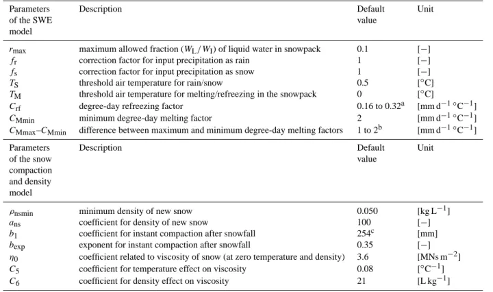
Table 1. The 15 seNorge snow model parameters with their default values and units. The values have been set on the basis of literature,
expert judgement as well as model evaluation against observations (see Engeset et al., 2004b).
Parameters Description Default Unit
of the SWE value
model
rmax maximum allowed fraction (WL/WI) of liquid water in snowpack 0.1 [−] fr correction factor for input precipitation as rain 1 [−] fs correction factor for input precipitation as snow 1 [−]
TS threshold air temperature for rain/snow 0.5 [◦C]
TM threshold air temperature for melting/refreezing in the snowpack 0 [◦C]
Crf degree-day refreezing factor 0.16 to 0.32a [mm d−1◦C−1] CMmin minimum degree-day melting factor 2 [mm d−1◦C−1] CMmax–CMmin difference between maximum and minimum degree-day melting factors 1 to 2b [mm d−1◦C−1]
Parameters Description Default Unit
of the snow value
compaction and density model
ρnsmin minimum density of new snow 0.050 [kg L−1]
ans coefficient for density of new snow 100 [−]
b1 coefficient for instant compaction after snowfall 254c [mm] bexp exponent for instant compaction after snowfall 0.35 [−] η0 coefficient related to viscosity of snow (at zero temperature and density) 3.6 [MNs m−2] C5 coefficient for temperature effect on viscosity 0.08 [◦C−1] C6 coefficient for density effect on viscosity 21 [L kg−1]
aCurrently parameterized as 0.08·C
M, whereCMvaries from 2 to 4 mm d−1◦C−1. bGrid cell specific default values are applied forC
Mmaxdepending on the latitude and forest cover (higher values above treeline) of the grid cell (Engeset et al., 2004b). cThe original equation in inch-units is converted to mm-units here (original value ofb
1is multiplied by 25.4).
2 Description of the seNorge snow model
In this section the equations in the seNorge snow model code (version 1.1) are presented. The model parameters and their default values are summarized in Table 1.
The seNorge snow model takes as input forcing the daily mean air temperatureT [◦C] and the daily sum of precip-itationP [mm]. The model consists of two main modules: (1) the SWE model for snow pack water balance, based on the snow routine in the HBV model (Sælthun, 1996), and (2) the snow compaction and density module (Alfnes, un-published NVE research note, 2008) used to convert SWE to SD. The SWE model for snow pack water balance is run before the snow compaction and density module.
2.1 SWE model for snowpack water balance
The precipitation is categorized as liquid or solid (PL,PS) de-pending on whetherT is above or below the snowfall thresh-old temperature parameterTS:
IfT ≤TS(conditions for snowfall)
PS =fS·P
PL =0. (1)
IfT > TS(conditions for rain)
PS =0
PL =fR·P , (2)
where the parametersfS andfR are correction factors for the input precipitation (as snow and rain, respectively). The degree-day factor CM for potential daily melting rate [mm d−1◦C−1] varies in the model seasonally as a sinus-wave betweenCMminandCMmaxreaching its maximum at the summer solstice (around 21 June):
CM =CMmin+((CMmax−CMmin)·0.5
·(sin(2π ((Nd−81.5) /366))+1)) , (3) whereNdis the number of the current day in the current year. Depending on whether T is above or below the melt-ing threshold temperature parameterTM, the potential daily melting (positive values) or refreezing (negative values)M∗
[mm d−1] in the snow pack is calculated. The actual daily melting or refreezingM[mm d−1] is restricted by the avail-ability of ice and liquid water in the snow pack, respectively:
IfT≤TM(conditions for refreezing)
M∗=Crf(T −TM) (4)
IfT > TM(conditions for melting)
M∗ =CM(T −TM) (6)
M=minM∗, WIt−1+PS
, (7)
where the superscripts t and t−1 denote values from the current (today’s) and previous (yesterday’s) time steps, and whereCrf[mm d−1◦C−1] is a degree-day factor for refreez-ing in the snowpack. The ice content in snow (in water equiv-alents)WI [mm], as well as the potential and actual liquid water contents in snow (WLpot andWL, [mm]) are updated correspondingly:
WLpott =WLt−1+PL+M (8)
WLt =minWLpott , rmax·WIt
(9)
WIt =WIt−1+PS−M, (10)
where rmax is the maximum allowed liquid water to ice weight ratio (WL/WI) in the snowpack, used to restrict the actual liquid water content in snow (WL).
Finally, SWE [mm] is the sum of liquid water and ice (in water equivalents) contained in the snow pack, and the dif-ference between potential and actual liquid water contents in the snow pack is lost to runoffQ[mm d−1]:
SWEt =WIt +WLt (11)
Q=WLpott −WLt. (12)
2.2 Snowpack compaction and density model
The snow compaction and density model algorithms in the seNorge model are adopted from the VIC model (Cherkauer and Lettenmaier, 1999) and from the SNTHERM model (Jor-dan, 1991). This part of the model calculates the changes in SD [mm] in three steps. In the first step, any net decrease in SWE since the previous time step (due to melting; not taking into account the new snow fallen at the current time step) is taken into account in the snow depth SD0 by reducing SD from the previous time step with the same relative amount: SD0=SDt−1·min
max SWEt −PS,0 SWEt−1 , 1
!
. (13)
In the second step, the lowering of the snow depth 1SD1 due to instant compaction of the old snowpack (i.e. com-paction only below the new snow fall) owing to weight of new snow fallen at the current time step (if any) is calculated as in Bras (1990):
1SD1= −
PS
SWEt −PS ·
SD 0
b1 bexp
·SD0, (14a) whereb1 andbexp are empirical coefficients (see Table 1). After the initial compaction and added new snow, snow depth SD1becomes thus:
SD1=SD0+1SD1+
min(SWE, PS)
ρns
, (14b)
whereρns is the density of new snow fallen at the current time step (if any). The value ofρnsis estimated as a function of air temperature as in Bras (1990):
ρns =ρnsmin+
max(T fahr,0)
ans
2
, (14c)
whereρnsminis the minimum density of new snow,ansis an empirical coefficient (see Table 1), andTfahr is the air tem-perature in Fahrenheit units, i.e.Tfahr=T ·9/5 + 32.
In the third step, a gradual compaction1SD2of the whole snow pack is calculated by making the assumption com-monly used in snow models that snow behaves as a viscous medium (e.g. Yen, 1981; Armstrong and Brun, 2008):
1SD2= −
kc·g·ρW·(0.001·SWE)
η0·exp(−C5·Tsnow+C6·ρ1)
·SD1·1t, (15a)
where the numerator describes the force [N m−2] due to the weight of the snowpack over the layer that compaction is cal-culated for, and the denominator the viscosity of the snow [Ns m−2] as a function of snow temperatureT
snow(estimated by min (T, 0)) and densityρ1= SWE/SD1. The kc, g and
ρWare the weight scaling constant (0.5), gravitation constant (9.81 m s−2) and water density (1000 kg m−3), respectively. Theη0,C5 andC6are empirical coefficients (see Table 1) and1t the time step (= 86 400 s). The final snow depth and density (SDt,ρt) for the present time step are then calculated as:
SDt =SD1+1SD2 (15b)
ρt = SWE
t
SDt . (15c)
3 Model evaluation
As pointed out in Sect. 1, previous studies have indicated that the seNorge snow model tends in general to overestimate both SWE andρ. In order to make a statistical and more de-tailed evaluation of the model performance along different covariates, such as elevation and the date in the snow sea-son (ts), two extensive sets of in situ snow measurements for Norway are applied. The first of the snow data sets consists of daily point measurements of SD recorded at stations op-erated by the met.no since 1882 (hereinafter referred to as the “met.no-data”). The second data set consists of measure-ments of SD andρ(enabling calculation of SWE) recorded at stations operated by various hydropower companies since 1914 (hereinafter referred to as the “HPC-data”). Since the seNorge snow map simulations start in 1 September 1957, data before that is not considered in the following sections. The spatiotemporal distribution and other features and dif-ferences of these two snow data sets are shown in Fig. 1 and listed in Table 2.
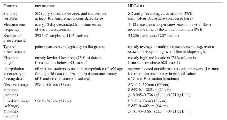
Table 2. Features of the two snow data sets used in the seNorge model evaluation (data since 1 September 1957 is considered). SD, SWE
andρdenote snow depth, snow water equivalent and bulk density, respectively, and “m a.s.l.” elevation (meters above sea level).
Features met.no-data HPC-data
Sampled SD (only values above zero, and stations with SD andρ(enabling calculation of SWE; variables at least 10 measurements considered here) only values above zero considered here)
Measurement every 10 days, extracted from time series 1–13 measurements per snow season, most of them frequency of daily measurements around the time of the annual maximum SWE Number of 392 547 samples at 1105 stations 32 256 samples at 1207 stations
measurements
Type of point measurement, typically on flat ground mostly average of multiple measurements, e.g. over a
measurements snow course spanning over different slope angles
Elevation mostly lowland locations (75 % of data is mostly highland locations (75 % of data is range∗ from stations below 480 m a.s.l.) from stations above 680 m a.s.l.)
Interpolation often same stations as used in interpolation of seNorge stations located outside met.no station network (i.e. more uncertainty in forcing grid-data (i.e. less interpolation uncertainty interpolation uncertainty in gridded values
forcing data ofT and/orPat station locations) ofT andP at station locations) Observed range, SD: 1–490 cm (32 cm) SD: 0.2–570 cm (100 cm)
min–max SWE: 0.1–285 cm (31 cm)
(median) ρ: 0.065–0.736 kg L−1(0.321 kg L−1)
Simulated range SD: 0–393 cm (33 cm) SD: 0–730 cm (129 cm)
(seNorge), SWE: 0–402 cm (54 cm)
min–max ρ: 0.143–0.667 kg L−1(0.421 kg L−1)
(median)
∗As a comparison: 60 % of the area of Norway is located below 600 m a.s.l., and 20 % above 900 m a.s.l.
While the met.no-data has one hundred times more obser-vations and a better spatiotemporal coverage than the HPC-data, ρ has not commonly been observed at the met.no-stations. This complicates model evaluation somewhat, since a good model fit in SD can result by compensating model biases, e.g. due to overestimation in both SWE andρ. The HPC-data, however, includes measurements of both SD and
ρ, which is an advantage in seNorge model evaluation. The met.no-data also represents point observations, while the HPC-data is based mostly on averages of several observa-tions taken over a snow course, which leads to smaller un-certainty in observing the grid cell mean snow conditions. Moreover, the potential model uncertainty due to input forc-ing should be less at the met.no-stations than generally in model grid cells, since data from the same met.no-stations are often used in the interpolation ofT and/orP to the model grid cells. Consequently, the model biases and uncertainties detected at the HPC-stations are probably more representa-tive for the majority of the seNorge model grid cells than those detected at the met.no stations. The melting season is, however, better resolved in the met.no-data. These and other sources of uncertainty are further discussed in Sect. 4. All the evaluation statistics were calculated using the “R” statistical software (www.r-project.org).
3.1 Model performance against snow data from met.no-stations
The met.no-data of daily SD measurements were down-loaded from the met.no climate data web service
(ek-lima.met.no/wsKlima). Measurements at 10-day intervals
were extracted from the original daily time series from 1957– 2011 for model evaluation purposes. Since it was difficult to separate between true SD zero-values (i.e. bare ground) and missing observations, all zero or negative values in the data set were replaced by missing values, and thus only posi-tive SD values were considered in the model evaluation. One clearly erroneous value was removed.
The simulated SD values in grid cells corresponding to the met.no-stations were extracted from the seNorge model re-sults, and only those grid cells where the difference between station and grid cell elevation was within ±100 m were used. After this matching, there were 392 547 observation-simulation pairs of SD at 1105 met.no-stations, which could be used in model evaluation (see Fig. 1 and Table 2). Of these, 107 267 (27 %) pairs had either the simulated or the observed SD≤10 cm. The number of observations varies be-tween 4000 and 10 000 per snow season for 1957–2011 and decreases strongly with elevation, as most of the met.no-stations are located in lowland regions (Fig. 1).
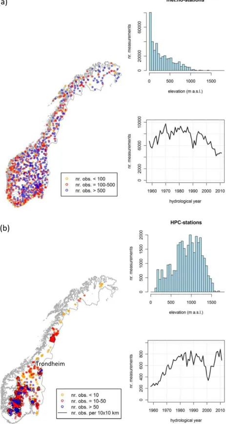
(a)
(b)
Trondheim
Fig. 1. Spatiotemporal distribution of the snow measurements in the (a) met.no-data (392 547 samples in total, varying from 10 to 1170 per
station) and (b) HPC-data (32 256 samples in total, varying from 1 to 239 per station) from 1957–2011. The colours in the map denote the number of observations per station, as indicated in the legend. The contours in (b) show the number of samples per 10×10 km grid cells (dashed contours denote 15 samples, solid contours 50, 100 and 150 samples), and the city of Trondheim marks the division line between southern and northern Norway.
between simulated and observed values. The R2 was 0.61 in the case of the original SD values and 0.56 in the case of the log10-transformed SD values. A spline-based gen-eral additive model (GAM) fitted to the cloud of points of observed vs. simulated SD (not shown) revealed, that the seNorge model fit switches from an overestimation for the lowest observed SDs below ca. 30 cm to a slight underesti-mation above that. However, since SD varies strongly with elevation, region and time of the snow season, it is important to analyse the differences between simulated and observed SD (1SD = SDsim−SDobs) further along these three main covariates.
The different percentiles of the1SD distribution alongts are shown in Fig. 2. This figure shows almost no systematic bias in1SD, until the main melting season from the mid-dle of March onwards, when the model starts to increasingly overestimate the observed SD. However, it is worth bearing in mind that only non-zero, positive SD values are used, and thus the number of observations varies strongly alongts, hav-ing a maximum around February, and behav-ing much lower both at the start and end of the snow season, as Fig. 2 shows. Moreover, the median station elevation is negatively corre-lated with the number of available observations, reaching a minimum elevation around February.
Since the variance of 1SD increases along ts, an al-ternative model fit measure was calculated, namely the relative difference (i.e. ratio) between simulated and ob-served SD (1SD∗= SDsim/SDobs). As Fig. 2 shows, the vari-ance of 1SD∗ is more constant along ts, except in the main melting season. Consequently, the relative difference model fit measure is preferred for SD and SWE in the fol-lowing model evaluations. Assuming that the station-wise log10(1SD∗) is normally distributed (visually confirmed), then Mean (log10(1SD∗))≈Median (1SD∗), and an 80 % confidence factor CF80% can be applied to describe the station-wise variability around the median value. For exam-ple, a CF80%(1SD∗)= 2 means that 80 % of the1SD∗ val-ues are between 1/2 and 2 times the median value.
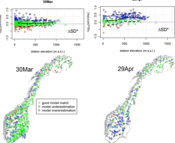
Figure 3 shows the spatial distribution (station position and elevation) of the station-wise Mean (log10(1SD∗)) for two selected dates alongts, for stations with measurements from at least 15 snow seasons. Those stations where the systematic bias is not detected to be statistically signifi-cantly larger than −23 to +30 % (corresponding to a fac-tor larger than 1.3 deviation from a “perfect match”) were categorized as “good match” stations. In addition, stations at each investigatedts (every 30 days from 30 December to 29 May) were binned by 200 m elevation intervals, and me-dian, 10 and 90 % percentiles of the station-wise means and variability were calculated for the bins containing at least 15 stations. These results show that from January through March the average station-wise Median (1SD∗) in all bins are within−14 to +22 % of the exact match, as the example for 30 March in Fig. 3 illustrates. At the end of April, how-ever, the station-wise Median (1SD∗) values are generally
positively biased, increasingly so at higher elevations (me-dian bias of +25 % in the 0–200 m a.s.l. bin, and +108 % in the 400–600 m a.s.l. bin, Fig. 3). Similarly, from January through March the average station-wise CF80%(1SD∗) is 1.3–2.3 (the lower the bin elevation, the higher the value), and at the end of April, somewhat higher (1.8–2.6). The per-centage of “good match” stations is 72–83 % before April, but decreases to 42 % at the end of April.
Figure 3 also shows the geographical distribution of the met.no-stations where SD is significantly systematically under- or overestimated (shown for 30 March and 29 April). No very distinct clustering patterns appear, except that no significant bias is detected at a majority of the stations in the eastern, more continental half of the southern Norway on 30 March (or before that; not shown), until the general over-estimation pattern starts to prevail from April onwards. 3.2 Model performance against snow data from the
HPC-stations
The HPC-data consists of measurements of SD andρ (en-abling estimation of SWE) taken by various hydropower companies since the 1910s. This data is managed by NVE, where the whole data set has recently been quality con-trolled by removing or correcting bad or duplicate values and outliers. Only data where both SD andρ were reported in the period 1957–2011 were used in model evaluation (SWE =ρ·SD). Most of the measurements (60 %) are taken once per snow season around the time of the maximum an-nual SWE (March–April), but at many stations several (up to 13) measurements per snow season have been taken. A snow measurement from an HPC-station is normally based on a snow course, but may also be based on a sample taken at one or more points at/around the station.
As in the case of the met.no-data (see previous section), zero SWE and SD values were removed from the data set (<1 % of the data), and the seNorge model-simulated SD and SWE values in grid cells corresponding to the HPC-stations were extracted, resulting in 32 256 observation-simulation pairs of SD, SWE and ρ at 1207 HPC-stations (see Fig. 1 and Table 2). The station elevation ranges from 139 to 1700 m a.s.l., with most of the observations located on the central mountain area in the southern Norway, and most of them (70 %) taken between 600–1300 m a.s.l. (Fig. 1). The number of observations varies between 200 and 900 per snow season from 1957–2011 (Fig. 1). Mostly the same methods as described in the previous section are also applied to model evaluation with the HPC-data.
(b)
(a)
ρ
Δ Δ
Δ Δ
Δρ ρ
(c)
Fig. 2. (a) Seasonal changes in the number of observations, in their median and 25/75 % percentile elevation, as well as in the observed median
snow depth (SD), snow water equivalent (SWE) and bulk snow density (ρ) in the met.no- and HPC-data from 1957-2011. The dashed line denotes the “low SD” subset of the met.no-data where the simulated and/or observed snow depth (SD) is<10 cm. (b) Seasonal changes in the median and 5, 25, 75 and 95 % percentiles of the distribution of the difference (1SD) and log10-transformed ratio (1SD∗) between the simulated and observed SD from 1957–2011 in the met.no-data. (c) Same as (b), but now for the HPC-data, for log10-transformed ratio (1SWE∗,1SD∗) between the simulated and observed SWE and SD, as well as for the difference (1ρ) between the simulated and observed
ρ. Only values based on at least 250 measurements (50 in HPC-data) per date are shown. Note that some of the 5 % percentile values in (b) are zero, and thus cannot be properly plotted on log-scale. The total number of observations in the figure is (b)∼392 000 and (c)∼32 000.
Δ
Δ
Fig. 3. Spatial distribution (with elevation and station position) of the station-wise mean log10-transformed ratio (1SD∗) between simulated and observed snow depth at two selected dates at met.no-stations from 1957–2011. The green, red and blue circles indicate stations with at least 15 years of observations, where the station-wise median1SD∗is not (green; “good match”), or is detected to be statistically significantly smaller (red; “underestimation”) or larger (blue; “overestimation”) than the threshold window of−23 to +30 % (corresponding to a factor larger than 1.3 deviation from a “perfect match”). A two-sided p-value<0.05 is applied as the significance level. In the upper panel, the solid and dashed lines denote the median and the 10/90 % percentiles of the station-wise means in each 200-m elevation bin, respectively. The total number of stations is 539 and 252 on 30 March and 29 April, respectively.
values of observedρ, indicating that the current density algo-rithm overestimates compaction the most at the lower density range.
As in the previous section, Fig. 2 shows the dif-ferent percentiles of the distribution of 1SD∗ and
1SWE∗(= SWEsim/SWEobs) along ts. The same every-10-day time resolution is used, as with the met.no-data. How-ever, since the HPC-data is not sampled daily, date-windows of 10 days around the dates intsare applied to bin together observations taken at almost the same dates. The number of stations varies strongly alongts, as Fig. 2 shows, peak-ing around late March and early April, i.e. at the time of the annual maximum SWE. The number of stations is much lower both at the start and end of the snow season, and thus the melting season is not well represented in this data (see Fig. 2).
Due to the lower number of stations, as well as variation in median elevation of the observations (Fig. 2), both1SD∗and
1SWE∗have a more ragged pattern alongtsthan the met.no data. The overall variance of1SD∗and1SWE∗seem to be rather invariant alongts, except during the main melting sea-son in April, when the 5 to 95 % percentile intervals increase markedly. The median of the difference between simulated and observed ρ (1ρ=ρsim−ρobs) reaches a maximum of +0.12 kg L−1 in early March, being somewhat smaller both at the beginning and end of the snow season (Fig. 2).
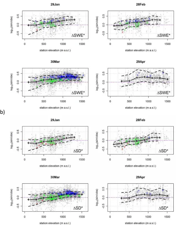
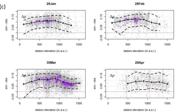
(a)
(b)
Fig. 4. Caption on next page.
increasing with elevation between roughly 500–1000 m a.s.l. For example, at 30 March the median bias is +34 and +100 % at the bins centered at 500 and 1100 m a.s.l., respectively. Due to overestimation inρ (median1ρ∼+0.1 kg L−1), the corresponding bias for 1SD∗ is somewhat less (−5 and +54 %, respectively). On 29 April, the significant bias in
1SWE∗ still remains above∼500 m a.s.l. (+50 to +100 %)
but does not show any clear trend with elevation anymore. The 10 and 90 % percentiles in Fig. 4 show the variabil-ity in model fit. On 30 March, for example, 80 % of all the simulated SWE values between 400–600 m a.s.l. are within −22 and +139 % of the observed SWE in the HPC-data, which corresponds to a CF80%of 1.7–1.8 around the median bias of +34 %. The percentage of “good match” HPC-stations
ρ
Δ Δ Δρ
(c)
Fig. 4. Median (solid lines) and 10/90 % percentiles (dashed lines) of the difference (grey dots) between the seNorge model-simulated and
observed (a) snow water equivalent (SWE), (b) snow depth (SD), and (c) bulk snow density (ρ) at four different dates in snow seasons 1957–2011 in the HPC-data. Statistics are calculated in 200 m elevation-bins (with at least 50 observations; centers of the bins are denoted by black “+” markers). The panels (a) and (b) show the relative log-transformed difference (1SD∗,1SWE∗) and (c) the absolute difference (1ρ). The coloured circles in (a) and (b) denote the stations with “good match” (green), “overestimation” (blue) and “underestimation” (red), as explained in Fig. 3.
(see definition in previous section) for SWE was 57 and 28 % in 28 February and 30 March, respectively.
The large-scale regional differences in 1SWE∗ were roughly investigated by removing all data in southern Nor-way (south of Trondheim; see Fig. 1). Although the data coverage in northern Norway is rather limited (5 % of all data), the results (not shown) did not indicate any less bias in SWE than seen in the whole dataset. A plot similar to Fig. 4 showed a median bias of +76 and +57 % at 30 March in ele-vation bins centered at 500 and 700 m a.s.l., respectively.
4 Discussion
There are several possible sources of uncertainty which can explain the differences seen between the simulated and ob-served snow conditions in the two previous sections. Firstly, there is the uncertainty connected to the seNorge model structure (process representation, subgrid variability), model parameters, and model input forcing (i.e. observations ofP
andT and their interpolation to grid cells). Secondly, there is the uncertainty connected to the rather substantial natu-ral spatial variability in snow conditions within the model 1×1 km grid-cells (see e.g. Clark et al., 2011), and to how well the point- and snow course-based measurements can capture this variability. Finally, there is also the uncertainty
connected to the snow observations, although this uncer-tainty is often relatively small when compared to the spatial variability, for example (except for density, which can some-times be demanding to measure).
As summarized in Table 2, the two data sets differ in many ways from each other. The HPC-data seems to give a more representative picture of the seNorge model fit in Norway in general than the met.no-data, since the interpo-lation uncertainty in the forcing data at the met.no-stations is likely smaller than in most of the other model grid cells (see Sect. 3). Moreover, since the met.no-data consist of point ob-servations, they have larger uncertainty in representing the grid cell mean snow conditions than the HPC-data, which is based mostly on averages over a snow course. On the other hand, due to less uncertainty in the forcing data, the met.no-data could provide a better basis for isolating the uncertainty connected to the model structure and parameters, had it not been for the fact that the lack of measurements ofρmakes the model evaluation more difficult, since a good fit for SD can arise from compensating biases in simulating SWE and
ρ.
to refining and quantifying the knowledge on the seNorge model performance by revealing the dependencies of the model fit by region, by the date of the snow season, and espe-cially by elevation. Although 60 % of the area of Norway is located below 600 m a.s.l., the higher elevation regions are of special interest (e.g. hydropower production). Since the pos-itive bias for SWE increases with elevation, it could be, as indicated by previous studies, that the elevation-dependency in the interpolation of the forcing data is too strong forP
and/orT, leading to increasingly excessive snow production along increased grid cell elevation. This explanation seems plausible, since most of the meteorological stations used in the interpolation are situated in the lowland areas, so that the interpolated values at the higher elevation sites become more uncertain. Other elevation-dependent processes (or lack thereof) responsible for the increasing bias along elevation could be, for example, the missing simulation of wind effects in the seNorge model, such as sublimation in blowing snow. Wind certainly also redistributes snow within a grid cell, but the transport of snow between the grid cells is probably neg-ligible. Armstrong and Brun (2008) reviewed some blowing snow model studies for Arctic regions, which showed that loss by sublimation could be 9 to 47 % of annual snowfall, depending on the topography and vegetation type. Thus, al-though sublimation could account for a fraction of the over-estimation in SWE it seemingly cannot alone explain losses of the order of what is shown in Fig. 4.
The evaluation results with the HPC-data indicate thatρ
is also overestimated in the lower elevations, thus indicating that the rather good model fit seen for the SD in the met.no-data might be coupled with an overestimation of SWE. How-ever, it is difficult to confirm this due to low number of low-land HPC-data, and since measurements ofρ are generally lacking below 200 m a.s.l., where the seasonal evolution of theρand SWE may be characterized by many accumulation and melting periods, and thus be different from the higher, more alpine and stable snow climate. The overestimation of
ρdoes not seem to be caused by the overestimation of SWE though (i.e. due to more overburden weight in the snow pack and thus more compaction), as the lacking coherence be-tween these variables in Fig. 4 indicates. Thus, adjustments to the snow compaction algorithm may be necessary in future model versions in order to correct these biases. In fact, pre-liminary model testing indicates that the second step in the compaction algorithm (1SD1in Eq. 14a) might be unneces-sary, causing some of the model density overestimation.
For comparison, we also tested whether an empirical sta-tistical snow density model, e.g. that of Sturm et al. (2010), would perform better than the more process-based density algorithm in the seNorge model. The model by Sturm et al. (2010), which estimates ρ as a function of snow cli-mate type (alpine assumed in our case), SD and the day of the year, showed less bias than the seNorge density model (+0.04 vs. +0.1 kg L−1), but the variability in ρ was still
better simulated in the seNorge model (R2= 0.45) than in the model by Sturm et al. (2010) (R2= 0.32).
In the melting season (as illustrated by the difference from 30 March to 29 April in Figs. 3 and 4) the spread in1SWE∗ increases in the HPC-data, while the bias approximately re-mains the same. For the met.no-data, the bias in1SD∗ in-creases during the melt season, and on 29 April the posi-tive bias increases also with elevation, which is not seen on 30 March (Fig. 3). This indicates that the positive bias here is due to model underestimation of the melting rates, since the bias in bulk density seems to be decreasing along the melting season (Fig. 4). There is also an indication for increased bias during the melting season in the HPC-data at the lower ele-vations below ca. 1000 m a.s.l. However, it is worth bearing in mind that the melting season is not as well represented in the HPC-data as in the met.no-data, and that the number of stations decreases strongly from the end of March to the end of April in the HPC-data.
Despite the rather substantial biases, the seNorge model describes rather well the variability in snow conditions, as theR2values indicate (53–60 % of the observed variance in log-transformed SWE and SD are explained by the model). One way of utilizing this strength of the model is to use the snow simulations in a relative sense, e.g. by calculating the ratio between current SWE in a grid cell and a correspond-ing long-term median SWE. In these relative units most of the systematic bias is removed. For example on 30 March, in the 1000–1200 m a.s.l. bin, the 80 % confidence range for
1SWE∗is +26 to +203 % (Fig. 4), while when using station-wise relative units (stations with at least 15 years of obser-vations included) the bias is removed and 80 % confidence range is now−28 to +38 % (similarly,−25 to +45 % in the lower 400–600 m a.s.l. bin).
As already pointed out above, the observational uncer-tainty is largest for the point observations, but neither a mean over a snow course can give a “true” mean of the snow conditions within, for example, a 1×1 km grid cell. Thus, even with a hypothetically perfect model, no perfect match with observations can be expected. Considerable spa-tial subgrid variability in SWE and SD is caused, among others, by local precipitation patterns and by wind redistri-bution of snow, which again is dependent on the type of vegetation and topography (e.g. Armstrong and Brun, 2008; Clark et al., 2011). As an example of the observational un-certainty, the high-resolution SD measurements across the Hardangervidda mountain plateau (Ragulina et al., 2011; see Sect. 1) showed that a single point measurement of SD has typically an 80 % confidence range of−60 to +70 % in es-timating the mean SD over 1 km subsections of the approx-imately 80 km long transects. By replacing the single point measurement by a mean over a snow course, (by taking a mean SD of 30 samples) the typical 80 % confidence range is reduced to±10 %. This example illustrates the generally better accuracy in the HPC-data, which is mostly based on snow courses, than in the point measurements of SD taken at
the met.no-stations. The confidence ranges in the above ex-ample apply for a treeless and hilly terrain over 1000 m a.s.l., and likely represent an upper range of variability in Norway, though. Subgrid variability in SD is likely somewhat smaller at the lower-lying met.no-stations, where the wind redistri-bution effect may be less pronounced and where the location of the snow stakes is fixed and can (in principle) be selected to be as representative as possible for the surrounding terrain. The high-resolution SD data from the transects across Hardangervidda (Ragulina et al., 2011) were also compared to the corresponding seNorge model-simulated values. The
1SD∗ values from this additional comparison were simi-lar to those calculated for the HPC-data in Sect. 3.2. This high-resolution SD data can also be used to illustrate the effect of bias correction: if the seNorge simulation results were corrected for the +54 % bias indicated by the HPC-data (on 30 March in the 1000–1200 m a.s.l. elevation bin), then the observed mean SD for the Hardangervidda transects from 2008, 2010 and 2011 were over-/underestimated by the seNorge model only by +5,−13 and −10 %, respectively. This also indicates that the averaging over several model grid cells reduces the variability in the model fit, as compared to the grid cell-wise evaluation results presented in this paper.
It is clear that the seNorge snow model needs at least a re-calibration, or maybe also revision of some of the algorithms, in order to increase the model performance and to properly remove the biases revealed in this study. In addition to the already indicated revisions of the input forcing data and of the compaction algorithm, also better representation of the effects of vegetation (especially forest canopy) on snow ac-cumulation, sublimation and melting, as well as the use of in-put data with higher temporal resolution in the model should be tested and evaluated.
A suitable model calibration method should be able to uti-lize the strengths of the two datasets (Table 2). Since it is possible that several different parameter combinations can give equally good model fit (the so-called equifinality prob-lem, see e.g. Beven, 2006), the calibration method should be able to search for all plausible combinations of the model pa-rameters that can give statistically optimal model fit with the observations, taking into account also the uncertainty con-nected to the observations. One method that has shown to be able to fullfill these calibration requirements is the Markov chain Monte Carlo simulation (e.g. Gamerman, 1999; Salo-ranta et al., 2009).
The data presented in this paper can serve as a bench-mark data set, against which new seNorge model calibrations and developments, or even new alternative model codes, can be tested and evaluated. In the future evaluation work, also other snow data sources, such as satellite images of snow-covered areas, high-resolution spatial SD distribution data from airborne laser-scanning, and high-resolution time-series of SWE and SD from snow pillows should be used. Moreover, the results presented in this paper can be used in intercomparison of the accuracies in different snow map
production methods. The seNorge snow mapping method is seemingly only applied in Norway at present, but it could relatively easily be applied and tested in other countries too, especially where rugged topography and lack of observa-tions hampers the regular use of interpolation and satellite-based snow mapping methods. The results in this paper can also provide an indirect evaluation of the griddedT andP
data used for model forcing, especially at the HPC-stations which are often located at higher elevations and far outside the met.no station network. A better coverage of stations measuringT andP, especially at the higher elevation sites, would likely contribute to more accurate input forcing data that would likely also increase the accuracy and precision of the simulated snow maps further.
While waiting for the revised/recalibrated version of the seNorge model (a natural next step from this study), the bias-corrected or relative seNorge simulation results are rec-ommended to be used, in order to increase the quality of the information on snow conditions from the snow maps of Norway.
5 Conclusions
Owing to the large spatiotemporal variability of snow condi-tions in the mountainous Norway, the snow maps simulated by the seNorge model provide probably the best overview of the current and past snow conditions for Norway in gen-eral. This snow map production method is relatively simple, not very data-demanding, yet still process-based and able to provide snow maps of high spatiotemporal resolution (daily, 1×1 km grid cell).
The statistical evaluation of the seNorge snow model against the two large and mostly non-overlapping datasets from the HPC- and met.no-stations has revealed and quan-tified the model performance, i.e. the variability and biases between the model simulations and the observations in the corresponding model grid cells. The HPC-data shows that the seNorge model generally overestimates SWE, and that the distribution of model fit for SWE shows a clear depen-dency on elevation throughout the season. Especially be-tween roughly 500–1000 m a.s.l. the model bias clearly in-creases (or becomes less negative) with elevation. Thus, for example, around 30 March, the model overestimates SWE on average by +34 % in the 400–600 m a.s.l. bin, while by 100 % in the higher elevation 1000–1200 m a.s.l. bin. There is no clear seasonal variation in the model fit with the HPC-data. Moreover, the seNorge model overestimatesρon aver-age by approximately +0.1 kg L−1, and there is only a mod-erate variation in the model fit along the snow season and elevation forρ.
the uncertainty in model results can be significantly reduced by using relative units where current SWE is expressed as a percentage or a fraction of a long-term median value. In these relative units the bias in the simulation results is mostly re-moved and in 80 % of the cases the model results match the observed SWE within a factor of roughly 1.5 in both direc-tions. By taking areal averages over several grid cells, these confidence intervals are further reduced.
Based on the model evaluation results, there are three rec-ommendations for further model development with which the quality of the seNorge model results (and thus of the snow maps for Norway) could be increased, namely: (1) revision and/or calibration of the density algorithms (Eqs. 13–15), in order to diminish the positive model bias in ρ, (2) cali-bration of the degree-day factorsCM, in order diminish the positive model bias in SD (and SWE) in the melting season, as seen especially in evaluation against the met.no-data, and (3) closer investigation of which elevation dependencies (or lack of them) in the model or forcing data could best explain and diminish the increasing positive model bias in SWE with elevation.
Acknowledgements. Very special thanks for the various
hy-dropower companies and for the Norwegian Meteorological Institute (met.no) for provision of data, as well as for the seNorge model and code developers, including Eli Alfnes, Jess Ander-sen, Rune Engeset, Ingjerd Haddeland, Zelalem Mengistu and Hans Christian Udnæs. Thanks also to Ragnar Ekker for helping downloading the data from met.no and to the two anonymous reviewers for their constructive comments on the manuscript.
Edited by: A. Klein
References
Alfnes, E.: Snow depth algorithms – compaction of snow, Unpub-lished research note, Norwegian Water Resources and Energy Di-rectorate (NVE), Oslo, Norway, 2008.
Anderson, E. A.: National weather service river forecasting sys-tem: Snow accumulation and ablation model, NOAA technical memorandum NWS HYDRO-17, US Dept. of Commerce, Silver Spring, CO, 1973.
Armstrong, R. L. and Brun, E.: Snow and climate, Cambridge Uni-versity Press, Cambridge, UK, 86–91, 2008.
Beven, K.: A manifesto for the equifinality thesis, J. Hydrol., 320, 18–36, 2006.
Borgstrøm, R. and Museth, J.: Accumulated snow and summer tem-perature – critical factors for recruitment to high mountain pop-ulations of brown trout (Salmo trutta L.), Ecol. Freshwater Fish, 14, 375–384, 2005.
Bras, R. L.: Hydrology: an introduction to hydrologic science, Addison-Wesley, Reading, MA, USA, 643 pp., 1990.
Cherkauer, K. A. and Lettenmaier, D. P.: Hydrologic effects of frozen soils in the upper Mississippi River basin, J. Geophys. Res., 104, 19599–19610, 1999.
Clark, M. P., Hendrikx, J., Slater, A. G., Kavetski, D., Anderson, B., Cullen, N. J., Kerr, T., Hreinsson, E. ¨O., and Woods, R. A.: Representing spatial variability of snow water equivalent in hy-drologic and land-surface models: A review, Water Resour. Res., 47, W07539, doi:10.1029/2011WR010745, 2011.
Dyrrdal, A. V.: An evaluation of Norwegian snow maps: simulation results versus observations, Hydrol. Res., 41, 27–37, 2010. Endrizzi, S.: Verification of the seNorge snow model in point mode.
Unpublished research note, Norwegian Water Resources and En-ergy Directorate (NVE), Oslo, Norway, 2010.
Engeset, R., Tveito, O. E., Alfnes, E., Mengistu, Z., Ud-næs, H.-C., Isaksen, K., and Førland, E. J.: Snow map system for Norway, XXIII Nordic Hydrological Conference, 8–12 August 2004, NHP report 48(1), http://senorge.no/ senorgeAux/NHC2004Tallinn SnowMapSystem Paper.pdf, last access: 7 November 2012, Tallinn, Estonia, 112–121, 2004a. Engeset, R., Tveito, O. E., Udnæs, H.-C., Alfnes, E., Mengistu,
Z., Isaksen, K., and Førland, E. J.: Snow map validation for Norway, XXIII Nordic Hydrological Conference, 8–12 Au-gust 2004, NHP report 48(1), http://senorge.no/senorgeAux/ NHC2004Tallinn SnowMapValidation Paper.pdf, last access: 7 November 2012, Tallinn, Estonia, 122–131, 2004b.
Gamerman, D.:Markov Chain Monte Carlo: Stochastic simulation for Bayesian inference, Chapman & Hall, London, UK, 1999. Jordan, R.: A one-dimensional temperature model for a snow cover:
Technical documentation for SNTHERM.89, Special Report 91-16, US Army Cold Regions Research and Engineering Labora-tory, Hanover, NH, 49 pp., 1991.
Lindstr¨om, G., Johansson, B., Persson, M., Gardelin, M., and Bergstr¨om, S.: Development and test of the distributed HBV-96 hydrological model, J. Hydrol., 201, 272–288, 1997.
Mohr, M.: New routines for gridding of temperature and precip-itation observations for “seNorge.no”, met.no note 08/2008, http://met.no/Forskning/Publikasjoner/Publikasjoner 2008/ filestore/NewRoutinesforGriddingofTemperature.pdf, last ac-cess: 7 November 2012, The Norwegian Meterological Institute, Oslo, Norway, 40 pp., 2008.
Mohr, M.: Comparison of versions 1.1 and 1.0 of gridded temper-ature and precipitation data for Norway, met.no note 19/2009, http://met.no/Forskning/Publikasjoner/Publikasjoner 2009/ filestore/note19-09.pdf, last access: 7 November 2012, The Norwegian Meterological Institute, Oslo, Norway, 44 pp., 2009. Ragulina, G., Melvold, K., and Saloranta, T.: GPR-measurements of
snow distribution on Hardangervidda mountain plateau in 2008– 2011, NVE-report 8-2011, Norwegian Water Resources and En-ergy Directorate, Oslo, Norway, 32 pp., 2011.
Saloranta, T. M., Forsius, M., J¨arvinen, M., and Arvola, L.: Impacts of projected climate change on the thermodynamics of a shal-low and a deep lake in Finland: Model simulations and Bayesian uncertainty analysis, Hydrol. Res., 40, 234–248, 2009.
Schreider, S. Y., Whetton, P. H., Jakeman, A. J., and Pittock, A. B.: Runoff modelling for snow-affected catchments in the Australian alpine region, eastern Victoria, J. Hydrol., 200, 1–23, 1997. Stenseth, N. C., Shabbar, A., Chan, K., Boutin, S., Rueness, E. K.,
Ehrich, D., Hurrell, J. W., Lingjærde, O. C., and Jakobsen, K. S.: Snow conditions may create an invisible barrier for lynx, P. Natl. Acad. Sci. USA, 101, 10632–10634, 2004.
Stranden, H. B.: Evaluering av seNorge: data versjon 1.1, Doku-ment no. 4/2010, http://www.nve.no/Global/Publikasjoner/ Publikasjoner%202010/Dokument%202010/dokument4-10.pdf, last access: 7 November 2012, Norges vassdrags-og energidirek-torat (NVE), Oslo, Norway, 36 pp., 2010.
Sturm, M., Taras, B., Liston, G. E., Derksen, C., Jonas, T., and Lea, J.: Estimating snow water equivalent using snow depth data and climate classes, J. Hydrometeorol., 11, 1380–1394, 2010. Sælthun, N. R. :The “Nordic” HBV model, Publication no. 7, The
Norwegian Energy and Water Resources Administration (NVE), Oslo, Norway, 26 pp., 1996.
Tahkokorpi, M., Taulavuori, K., Laine, K., and Taulavuori, E.: After-effects of drought-related winter stress in previous and cur-rent year stems of Vaccinium myrtillus L., Environ. Exp. Bot., 61, 85–93, 2007.
Tveito, O. E., Udnæs, H.-C., Mengistu, Z., Engeset, R., and Førland, E. J.: New snow maps for Norway, Proceedings XXII Nordic Hy-drological Conference 2002, 4–7 August 2002, http://senorge.no/ senorgeAux/NHC2002Roros NewSnowMap Paper.pdf, last ac-cess: 7 November 2012, Røros, Norway, 527–532, 2002. Tveito, O. E., Bjørdal, I., Skjelv˚ag, A. O., and Aune, B.: A
GIS-based agro-ecological decision system GIS-based on gridded clima-tology, Meteorol. Appl., 12, 57–68, 2005.