Available online at www.ispacs.com/cna
Volume 2016, Issue 2, Year 2016 Article ID cna-00276, 7 Pages doi:10.5899/2016/cna-00276
Research Article
Numerical study of nonlinear singular fractional differential
equations arising in biology by operational matrix of shifted
Legendre polynomials
D. Jabari Sabeg1, R. Ezzati1∗
(1)Department of Mathematics, Karaj Branch, Islamic Azad University, Karaj, Iran.
Copyright 2016 c⃝D. Jabari Sabeg and R. Ezzati. This is an open access article distributed under the Creative Commons Attribution License, which permits unrestricted use, distribution, and reproduction in any medium, provided the original work is properly cited.
Abstract
In this paper, we present a new computational method for solving nonlinear singular boundary value problems of fractional order arising in biology. To this end, we apply the operational matrices of derivatives of shifted Legendre polynomials to reduce such problems to a system of nonlinear algebraic equations. To demonstrate the validity and applicability of the presented method, we present some numerical examples.
Keywords:Fractional differential equation, Operational matrix, Collocation method, Legendre polynomials.
1 Introduction
For modeling many physiology problems such as study of steady state oxygen-diffusion in a cell with Michaelis-Menten uptake kinetics [1, 2] bending of beams [3] and spring mass system [4], nonlinear differential equations are considered as essential instruments. These equations are also useful in study of the distribution of heat sources in the human head [5, 6] and tumor growth [7, 8, 9, 10, 11].
As we know, singular boundary value problems
y′′(x) + (a+m
x)y
′
(x) = f(x,y), 0≤x≤1, (1.1)
with the initial conditions
α1y(0) +β1y ′
(0) =A, (1.2)
α2y(1) +β2y ′
(1) =B, (1.3)
arise in physiology, where f(x,y)is continuous, ∂∂yf exists and is continuous and also ∂∂yf ≥0, 0≤x≤1. these problems, withm=0,1,2 anda=0, arise in the study of various tumor growth problems with linear f(x,y), and also, with non-linear f(x,y)of the form f(x,y) = f(y) =y+nyη, n>0, η>0 andm=2, a=0 arise in the study of steady state oxygen diffusion in a spherical cell with Michaelis-Menten uptake kinetics. A similar equation form=2
anda=0 arise in the study of the distribution of heat sources in the human head, in whichf(x,y) = f(y) =−δe−εy,
δ>0, ε>0. In this paper we generalize the definition of Eqs. (1.1)-(1.3) up to fractional order as following:
Dαy(x) + (a+m
x)D
βy(x) = f(x,y),
0≤x≤1, 1<α≤2, 0<β ≤1, (1.4)
α1y(0) +β1y ′
(0) =A, (1.5)
α2y(1) +β2y ′
(1) =B, (1.6)
whereA,Bare constants, f(x,y)is a continuous real-valued function. The main objective of this paper is to provide an introduction of a novel-method based on operational matrices of fractional derivative of shifted Legendre polyno-mials that have been demonstrated in [12] in order to solve equations (1.4)-(1.6). The main characteristic behind the approach using this technique is that it reduces these problems to those of solving a system of algebraic equations. The rest of the paper is organized as follows: In section 2, we present some necessary definitions and mathematical preliminaries of the fractional calculus theory and shifted Legendre polynomials which are required for establishing our results. In Section 3 the shifted Legendre operational matrix of fractional derivative is introduced. Section 4 is devoted to applying the shifted Legendre operational matrix for the problems given in Eqs (1.4)-(1.6). In Section 5, we solve some numerical examples by using the proposed method in previous section. Finally section 6, concludes the paper.
2 Preliminaries and notations
Here, we recall some basic definitions and properties of fractional calculus that are used in this article. There are various definitions of fractional integration and differentiation, such as Grunwald-Letnikov’s definition and Riemann-Liouville’s definition. The Riemann-Liouville derivative has certain disadvantages when trying to model real-world phenomena with fractional differential equations. Therefore, we will introduce a modified fractional differential operatorDαproposed by Caputo in his work on the theory of viscoelasticity [13].
Definition 2.1. The Caputo fractional derivatives of orderαis defined as
Dαf(x) = 1
Γ(n−α)
∫ x
0
f(n)(t)
(x−t)α−n+1dt, n−1<α≤n,n∈N,
whereα>0is the order of the derivative and n is the smallest integer greater thanα. For the Caputo derivative we have: [14]
Dαxβ =
0, f orβ∈N0andβ <⌈α⌉,
Γ(β+1)
Γ(β+1−α)xβ−α, f orβ∈N0andβ ≥ ⌈α⌉orβ∈/Nandβ >⌊α⌋,
Dαc=0, (c is a constant).
We use the ceiling function⌈α⌉to denote the smallest integer greater than or equal toα, and the floor function⌊α⌋ to denote the largest integer less than or equal toα. AlsoN={1,2, ...}and N0={0,1,2, ...}. Recall that forα∈N, the Caputo differential operator coincides with the usual differential operator of an integer order.
2.1 Shifted Legendre polynomials
The well-known shifted Legendre polynomials of orderiare defined on the interval[0,1]and satisfy in the fol-lowing recursive formula:
pi+1(x) =
(2i+1)(2x−1) (i+1) pi(x)−
i
wherep0(x) =1 andp1(x) =2x−1. The analytic form of the shifted Legendre polynomial pi(x) of degreei is given
by
pi(x) = i
∑
k=0
(−1)i+k (i+k)!x k
(i−k)!(k!)2. (2.7)
For these polynomials, by using orthogonality properties, we have:
∫ 1 0
pi(x)pj(x)dt=
1
2i+1, f or i=j,
0, f or i̸=j.
A functiony(x)∈L2[0,1]may be expressed in terms of shifted Legendre polynomials as
y(x) =
∞
∑
j=0
cjpj(x),
where the coefficientscjare given bycj= (2j+1) ∫1
0 pj(x)y(x)dx.
In practice, only the first(m+1)terms shifted Legendre polynomials are considered. Therefore,y(x)can be written in the form
y(x)≃
m
∑
j=0
cjpj(x) =CTB(x), (2.8)
where
CT = [c0,c1, ...,cm], (2.9)
B(x) = [p0(x),p1(x), ...,pm(x)]T. (2.10)
3 Operational matrix of derivative and fractional calculus
The derivative of the vectorB(x)can be expressed by
dB(x)
dx =D
(1)B(x), (3.11)
whereD(1)is the(m+1)×(m+1)operational matrix of derivative given by
D(1)= (di j) =
2(2j+1), f or j=i−k,
k=1,3, ...,m, i f m odd,
k=1,3, ...,m−1, i f m even,
0, otherwise.
By using Eq. (3.11), it is clear that
dnB(x)
dxn = (D
(1))nB(x), (3.12)
wheren∈Nand the superscript, inD(1), denote matrix powers.Thus
(D(1))n=D(n), n=1,2, . . . . (3.13) LetB(x)be shifted Legendre vector defined in (2.10), so supposeα>0 so,
whereD(α) is the(m+1)×(m+1)operational matrix of fractional derivative of orderα in the Caputo sense and is defined as follows [12]:
D(α)=
0 0 . . . 0
..
. ... . . . ...
0 0 . . . 0
∑⌈kα=⌉⌈α⌉θ⌈α⌉,0,k ∑⌈
α⌉
k=⌈α⌉θ⌈α⌉,1,k . . . ∑⌈
α⌉
k=⌈α⌉θ⌈α⌉,m,k
..
. ... . . . ...
∑ik=⌈α⌉θi,0,k ∑ik=⌈α⌉θi,1,k . . . ∑ik=⌈α⌉θi,m,k
..
. ... . . . ...
∑mk=⌈α⌉θm,0,k ∑mk=⌈α⌉θm,1,k . . . ∑mk=⌈α⌉θm,m,k
, (3.15)
whereθi,j,kis given by
θi,j,k= (2j+1) j
∑
l=0
(−1)(i+j+k+l)(i+k)!(l+j)!
(i−k)!k!Γ(k−α+1)(j−l)!(l!)2(k+l−α+1). (3.16)
4 Description of the method
A computational approach based on the operational matrix of derivative of shifted Legendre polynomials is of-fered in this section in order to solve nonlinear singular boundary value problem (1.4) with the mixed conditions (1.5) and (1.6). Clearly, from Eq. (2.8), we can approximate the solution of (1.4),y(x), as follows:
y(x) =CTB(x), (4.17) whereCandB(x)are defined in Eqs. (2.9) and (2.10). Also, by using Eq. (3.15), we conclude that
Dαy(t) =CTD(α)B(x), (4.18)
Dβy(t) =CTD(β)B(x). (4.19) Now, by substituting Eqs. (4.17), (4.18) and (4.19) in Eq. (1.4) we have:
CTD(α)B(x) + (a+m
x)C
TD(β)B(x) =f(x,CTB(x)). (4.20)
Also, by using Eqs. (1.5), (1.6), (3.13) and (4.17), we conclude that
α1CTB(0) +β1CTD(1)B(0) =A, (4.21)
α2CTB(1) +β2CTD(1)B(1) =B. (4.22)
To find the solutiony(x), we first collocate Eq. (4.20) at(m−1)points. To this end, we choose suitable collocation points as the first(m−1)shifted Legendre roots ofpm+1(x). Eq. (4.20) together with Eqs. (4.21) and (4.22) generate (m+1)nonlinear equations which can be solved using Newton’s iterative method. Consequently, we can obtainy(x)
given in Eq. (4.17).
5 Numerical examples
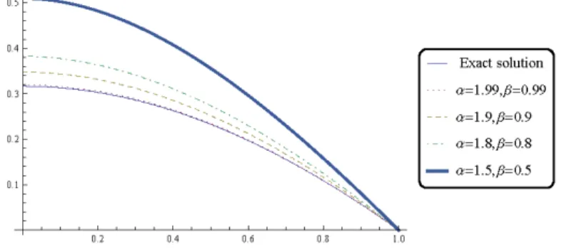
Example 5.1. As the first example, we Consider the following singular two point boundary value problem:
y(α)(x) +1
xy
(β)(x) =−ey, 1<α≤2, 0<β≤1, (5.23)
y′(0) =0, y(1) =0,
forα=2, β =1the exact solution is y(x) =2ln( 4−2√2
(3−2√2)x2+1). The approximate solution for m=15is graphically shown in Figure 1.
Figure 1: Comparison of the behavior ofy(x)form=15, with exact solution, for Example 5.1.
Example 5.2. Consider the following singular two point boundary value problem:
yα(x) + (1+1
x)y
β(x) =5x3(5x3ey−5−x)
4+x5 , (5.24)
y(0) =ln(1
4), y(1) +5y
′(1) =ln(1
5)−5.
forα =2, β =1, the exact solution of this example is y(x) =ln( 1
4+x5), The approximate solution for m=15is graphically shown in Figure 2.
6 Conclusion
In this paper, first, we introduced nonlinear singular boundary value problems of fractional order arising in biology. Then, we applied the shifted Legendre polynomials as the basis to solve these problems. By use of the operational matrices of derivatives of these basic functions, we converted such problems to an algebraic system. Finally, by solving this algebraic system, we presented the approximate solution of the problem.
Acknowledgements
The authors thank referee and editor for their useful technical comments and valuable suggestions to improve the readability of the paper, which led to a significant improvement of the paper.
References
[1] H. S. Lin, Oxygen diffusion in a spherical cell with nonlinear oxygen uptake Kinetics, J. Theor. Biol, 60 (1976) 449457.
http://dx.doi.org/10.1016/0022-5193(76)90071-0
[2] D. L. S. McElwain, A re-examination of oxygen diffusion in a spherical cell with Michaelis-Menten oxygen uptake Kinetics, J. Theor.Biol, 71 (1978) 255-263.
http://dx.doi.org/10.1016/0022-5193(78)90270-9
[3] S. S. Ganji, A. Barari, D. D. Ganji, Approximate analysis of two-mass-spring systems and buckling of a column, Computers and Mathematics with Applications, 61 (2011) 1088-1095.
http://dx.doi.org/10.1016/j.camwa.2010.12.059
[4] J. B. Paiva, A. V. Mendona, A coupled boundary element differential equation method formulation for platebeam interaction analysis, Engineering Analysis with Boundary Elements, 34 (2010) 456-462.
http://dx.doi.org/10.1016/j.enganabound.2009.10.017
[5] U. Flesch, The Distribution of heat sources in the human head: A theoretical consideration, J. Theor. Biol, 54 (1975) 285-287.
http://dx.doi.org/10.1016/S0022-5193(75)80131-7
[6] B. F. Gray, The Distribution of heat sources in the human head: A theoretical consideration, J. Theor. Biol, 82 (1980) 473-476.
http://dx.doi.org/10.1016/0022-5193(80)90250-7
[7] A. D. Conger, M. C. Ziskin, Growth of mammalian multicellular tumor spheroids, Cancer Res, 43 (1983) 556-60. [8] J. A. Adam, A simplified mathematical model of tumor growth, Math. Biosci, 81 (1986) 224229.
http://dx.doi.org/10.1016/0025-5564(86)90119-7
[9] J. A. Adam, A mathematical model of tumor growth II: effect of geometry and spatial non-uniformity on stability, Math. Biosci, 86 (1987) 183-211.
http://dx.doi.org/10.1016/0025-5564(87)90010-1
[10] J. A. Adam, S. A. Maggelakis, Mathematical model of tumor growth IV: effect of necrotic core, Math. Biosci, 97 (1989) 121-136.
http://dx.doi.org/10.1016/0025-5564(89)90045-X
[11] A. C. Burton, Rate of growth of solid tumor as a problem of diffusion, Growth, 30 (1966) 157-176.
[13] M. Caputo, Linear models of dissipation whose Q is almost frequency independent. Part II, J. Roy Austral. Soc, 13 (1967) 529-539.
http://dx.doi.org/10.1111/j.1365-246X.1967.tb02303.x
[14] K. Diethelm, N. J. Ford, A. D. Freed, Yu. Luchko, Algorithms for the fractional calculus: A selection of numer-ical methods, Comput. Methods Appl. Mech. Eng, 194 (2005) 743-73.