Numerical Solution of a Fractional Order Model of HIV Infection of CD4+T Cells Using Müntz-Legendre Polynomials

Numerical Solution of a Fractional Order Model

of HIV Infection of CD4

T Cells

Using Müntz-Legendre Polynomials

Mojtaba Rasouli Gandomani,M. Tavassoli Kajani*

Department of Mathematics

Isfahan (Khorasgan) Branch, Islamic Azad University Isfahan, Iran

E-mails: mojtabamath@yahoo.com, tavassoli_k@yahoo.com

*_{Corresponding author}

Received: November 29, 2015 Accepted: February 15, 2016

Published: June 30, 2016

Abstract: In this paper, the model of HIV infection of CD4+T cells is considered as a system of fractional differential equations. Then, a numerical method by using collocation method based on the Müntz-Legendre polynomials to approximate solution of the model is presented. The application of the proposed numerical method causes fractional differential equations system to convert into the algebraic equations system. The new system can be solved by one of the existing methods. Finally, we compare the result of this numerical method with the result of the methods have already been presented in the literature.

Keywords: HIV infection model, Fractional ODE, Müntz-Legendre polynomials, Collocation Method.

Introduction

The human immunodeficiency virus (HIV) is a lentivirus (a subgroup of retrovirus) which has a roughly spherical shape and a diameter of about 120 nm (about 60 times smaller than the dimension of red blood cell). It attacks the immune system of the body. Without a strong immune system, the body can not fight against cancers or other infectious diseases effectively. HIV infects and destroys certain white blood cells called CD4+T cells which are an important part of the immune system. If too many CD4+ cells are destroyed, the body is not perfectly capable of defending against infection. The fact is that the early and timely treatment can slow or stop progress of HIV infection. The medicines can help the immune system return to a healthier condition. The number of infected and uninfected CD4+T cells is important to measure HIV progress and to get best treatment and cure [5, 12].

Recently, different mathematical models are presented to examine the dynamics of CD4+T cells. The model in [27] is one of them with a system of differential equations as follows:

        

       

dT(t)

dt =q−ηT(t) +rT(t)

1−T(t) +1 Tmax

−kV(t)T(t)

dI(t)

dt =kV(t)T(t)−βI(t) dV(t)

dt =µβI(t)−γV(t)

T(0) =T0, I(0) =I0, V(0) =V0

Table 1. List of variables and parameters [2, 19, 21, 27]

Parameters and variables Meaning

T(t) The concentration of uninfected CD4+T in the blood

I(t) The concentration of infected CD4+T in the blood

V(t) The concentration of HIV virus particle in the blood

η Turnover rate of uninfected CD4+T cells

β Turnover rate of infected CD4+T cells

γ Turnover rate of HIV virus particles 1−T+1

Tmax Logistic growth indicator of uninfected CD4

+_{T cells}

k The infection rate of CD4+T cells by HIV virus

kV T The incident of HIV infection of healthy CD4+T

µ The number of virus particles produced by each infected CD4+T cell during its life time

q The generation rate of uninfected CD4+T cells in the body

µβ The generation rate of virions through infected CD4+T cells

Tmax The maximal concentration of CD4+T cells in the blood r Tate of cells’ duplication through the process of mitosis when

they are stimulated by antigen and mitogen

Ongum [20] has solved it by using Adomian Laplace decomposition. Srivastava et al. [23] have presented an accurate approximate solution of the differential equations system with a numerical method based on DTM. Yuzbasi [28] employs Bessel polynomials to find a numerical method for approximating the solution of the differential equations.

In recent years, the application of fractional differential equations has been found in different fields of sciences as well as in many scientific and practical models [10, 15]. Fractional differen-tial equations are applied in many natural phenomena in which case these equations have more validity and adaptation to the natural phenomena. Biological systems have fractal structures and they have very close ties with fractional differential equations [24, 25, 26]. Thus using frac-tional differential equations for these systems can produce more natural results. For instances, by using fractional differential equations, Arafa et al. [1] examined the impact of antiretroviral drugs and Erturk et al. [8] considered a model of kind of human virus which can infect CD4+T cells. Other applications of fractional differential equations are demonstrated in [6, 14, 22].

In this paper we consider the presented model in Eq. (1) as a form of fractional differential equations so the model changes as follows:

    

   

Dα1

∗ T(t) =q−ηT(t) +rT(t)

1−T(_Tt_max)+1−kV(t)T(t),

Dα2

∗ I(t) =kV(t)T(t)−βI(t),

Dα3

∗ V(t) =µβI(t)−γV(t),

T(0) =T0, I(0) =I0, V(0) =V0,

0≤t≤R<∞_,

0<α₁,α₂,α₃≤1,

(2)

where we adopt Caputo’s formula to obtain fractional derivative as follows:

Dα_∗y(t) = 1 Γ_(1−α)

Rt

0(t−τ)−αy′(τ)dτ.

differential equations. For more details one can read [7, 13, 18, 29].

In this paper, our aim is to solve fractional differential equations (2) system with a colloca-tion method based on the Müntz-Legendre polynomials. Since fraccolloca-tional derivative from a polynomial with integer order is not necessarily a polynomial with integer order so it is better to use collocation method based on polynomials with fractional order. The main advantage of using the Müntz-Legendre polynomials is that they have fractional order and actually their fractional derivative is also a Müntz-Legendre polynomial with the result that the use of the Müntz-Legendre polynomials in collocation method seems logical. Esmaeili et al. [9] used the Müntz-Legendre polynomials to solve fractional differential equations.

The paper is organized as follows: Section 2 is devoted to preliminaries. In fact this section contains two subsections. In the first one we introduce Jacobi polynomials. The second one is related to Müntz-Legendre polynomials. The collocation method to solve fractional differential equations system is presented in section 3. In section 4, the results are compared. Section 5 concludes the paper.

Preliminaries

Jacobi polynomials

The Jacobi polynomials are extensively used for solving fractional differential equations. They are orthogonal on the interval[−1, 1]with respect to the weight function

w(α,β)(t) = (1−t)α(1+t)β,

whereα,β >−1.

These polynomials can be obtained through the following recurrent relation:

J₀(α,β)(t) =1, J₁(α,β)(t) = 1

2((α−β) + (α+β+2)t),

a_k(α,β)J_k(₊α,β₁)(t) =b(_kα,β)(t)J_k(α,β)(t)−c_k(α,β)J_k(₋α,β₁ )(t),

a(_kα,β)=2(k+1)(k+α+β+1)(2k+α+β),

b(_kα,β)(t) = (2k+α+β+1)((2k+α+β)(2k+α+β+2)t+α2−β2),

c(_kα,β)=2(k+α)(k+β)(2k+α+β+2).

(3)

The initial derivative of the Jacobi polynomials can be obtained as follows:

d dtJ

(α,β)

k (t) =

1

2(k+α+β+1)J

(α+1,β+1)

k−1 (t). (4)

Müntz-Legendre polynomials

LetΛ_n={λ1,λ2,. . ._,λ_n}be under condition Re(λ_k)>−1

polyno-mials on the interval (0, 1] are defined as follows [3, 17]:

Ln(t) =L(Λn,t) = n

∑

Cn,ktλn, Cn,k= n−1

∏

(λk+λv+1)

n

∏

(λk−λv)

. (5)

Basic properties of the Müntz-Legendre polynomials:

(Ln,Lm) =

Z 1

0

Ln(t)Lm(t)dt =

δmn

λn+λn+1

,

Ln(1) =1,

L′_n(1) =λn+ n−1

∑

(λk+λk+1).

(6)

Here, allλ_kare chosen so thatλ_k=αk(αis a positive real number), the shifted Müntz-Legendre polynomials on the intervalI= [0,R)are defined as follows :

LI,n(t:α) = n

∑

Cn,k

t

R

αk

, Cn,k =

(−1)n−k

αn_k!(n−k)! n−1

∏

((k+v)α+1). (7)

Some of the shifted Müntz-Legendre polynomials’ properties according to [3] are:

LI,n(R:α) =1, L′I,n(R:α) =

αn+∑n_k=−1₀(2αk+1)

R .

Regarding Eq. (6), we have:

Z R

0

LI,n(t)LI,m(t)dt=

Rδmn

1+2αn.

Furthermore, following [13] a stable recurrence relation can be obtained for shifted Müntz-Legendre polynomials via the Jacobi polynomials, as follows:

LI,0(t:α) =1, LI,1(t:α) =

1

α +1

t R α − 1 α,

aI,nLI,n+1(t:α) =bI,n(t)LI,n(t:α)−cI,nLI,n−1(t:α),

aI,n=a

(0,_α1−1)

n , bI,n(t) =b

(0,_α1−1)

n

2 _Rtα−1, cI,n=c

(0,_α1−1)

n .

(8)

In addition, according to [17] fractional derivative of these polynomials can also be obtained with the following equation:

Dα_∗LI,n(t:α) =

1+αn

αΓ_(1−α)Rα

Z R

0 (1−

τα1)−α_J(1, 1 α)

n−1

2

t

R

α

τ−1

Method of solution

This section is devoted to presentation of the numerical method for evaluating fractional differ-ential equations system. Assumeα1=α2=α3=α. We approximate the unknown functions

of T(t), I(t), V(t), by using a linear combination of the shifted Müntz-Legendre function as follows:

T(t)≈Tn(t) = N

∑

cjLI,j(t:α),

I(t)≈In(t) = N

∑

djLI,j(t :α),

V(t)≈Vn(t) = N

∑

ejLI,j(t :α),

(10)

where coefficientscj,dj,ej, j=0, 1, 2,. . ., N are unknown. Now substituting Eq. (10) into the

fractional differential equations system Eq. (2) gives the following results:

                                                           N

∑

cjDα∗1LI,j(t :α) =q−η N

∑

cjLI,j(t :α)

+r∑N_j=0cjLI,j(t :α)

      1− N

∑

cjLI,j(t:α) +1

Tmax       −k N

∑

ejLI,j(t:α) N

∑

cjLI,j(t:α),

N

∑

djDα∗2LI,j(t :α) =k N

∑

ejLI,j(t:α) N

∑

cjLI,j(t:α)−β N

∑

djLI,j(t:α),

N

∑

ejDα∗3LI,j(t :α) =µβ N

∑

djLI,j(t:α)−γ N

∑

ejLI,j(t :α),

N

∑

cjLI,j(0:α) =T0, N

∑

djLI,j(0:α) =I0, N

∑

ejLI,j(0:α) =V0.

(11)

The fractional derivative of the above Legendre functions is obtained via Eq. (9).

Now, the collocation points θi, i=1, 2, . . ., nshould be substitute into Eq. (11). It is a fact,

that the best and simplest choice for the collocation points θi is Chebyshev points associated

with the interval[0,R]which is defined as follows:

θi=

R 2− R 2cos πi n

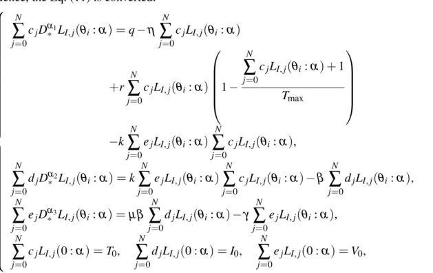
Hence, the Eq. (11) is converted:                                                              N

∑

cjDα∗1LI,j(θi:α) =q−η N

∑

cjLI,j(θi:α)

+r

N

∑

cjLI,j(θi:α)

      1− N

∑

cjLI,j(θi:α) +1

Tmax       −k N

∑

ejLI,j(θi:α) N

∑

cjLI,j(θi:α),

N

∑

djDα∗2LI,j(θi:α) =k N

∑

ejLI,j(θi:α) N

∑

cjLI,j(θi:α)−β N

∑

djLI,j(θi:α),

N

∑

ejDα∗3LI,j(θi:α) =µβ N

∑

djLI,j(θi:α)−γ N

∑

ejLI,j(θi:α),

N

∑

cjLI,j(0:α) =T0, N

∑

djLI,j(0:α) =I0, N

∑

ejLI,j(0:α) =V0,

(12)

Finally, Eq. (12) generates a system of 3n+3 algebraic equations with 3n+3 unknown coeffi-cients which can be solved by one of the existing methods and unknown coefficoeffi-cientscj,dj,ej,

j=0, 1, 2,. . .,nshould be obtained. Subtitling these coefficients in Eq. (10), we obtainT_n(t), In(t)andVn(t).

Numerical results

We employed Maple 16 software to find approximate solution.

In this section, we use the presented numerical method to solve the fractional differential equa-tions system Eq. (2). Besides, we consider the initial values and the explained parameters of the model as follows:

T0=0.1, I0=0, V0=0.1, q=0.1, η=0.02, β =0.3,

r=3, γ =2.4, k=0.00027, Tmax=1500, µ =10.

First, we use the presented method for α =1 and then we compare the obtained results with those of previous methods (See Tables 2, 3 and 4).

Table 2. Numerical comparison forT(t).

t LADM-Pade [20] Method in [28] VIM [16] RK4 Present Method

0.0 0.1 0.1 0.1 0.1 0.1

0.2 0.2088072731 0.2038616561 0.2088073214 0.2088080833 0.208808084 0.4 0.4061052625 0.3803309335 0.4061346587 0.4062405393 0.406240543 0.6 0.7611467713 0.6954623767 0.7624530350 0.7644238890 0.766442390 0.8 1.3773198590 1.2759624442 1.3978805880 1.4140468310 1.414046852 1.0 2.3291697610 2.3832277428 2.5067466690 2.5915948020 2.591559480

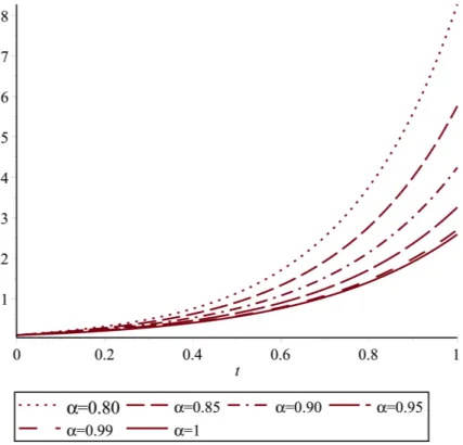
Figs. 1, 2 and 3, respectively demonstrate T(t), I(t) and V(t) using proposed method for

Table 3. Numerical comparison forI(t).

t LADM-Pade [20] Method in [28] VIM [16] RK4 Present Method

0.0 0 0 0 0 0

0.2 0.603270728e-5 0.6247872100e-5 0.6032634366e-5 0.6032702150e-5 0.603270224e-5 0.4 0.131591617e-4 0.1293552225e-4 0.1314878543e-4 0.1315834073e-4 0.131583409e-4 0.6 0.212683688e-4 0.2035267183e-4 0.2101417193e-4 0.2122378506e-4 0.212237854e-4 0.8 0.300691867e-4 0.2837302120e-4 0.2795130456e-4 0.3017741955e-4 0.301774201e-4 1.0 0.398736542e-4 0.3690842367e-4 0.2431562317e-4 0.4003781468e-4 0.400378155e-4

Table 4. Numerical comparison forV(t)

t LADM-Pade [20] Method in [28] VIM [16] RK4 Present Method

0.0 0.1 0.1 0.1 0.1 0.1

0.2 0.06187996025 0.06187991856 0.06187995314 0.06187984331 0.061879843 0.4 0.03831324883 0.03829493490 0.03830820126 0.03829488788 0.038294888 0.6 0.02439174349 0.02370431860 0.02392029257 0.02370455014 0.023704550 0.8 0.009967218934 0.01467956982 0.01621704553 0.01468036377 0.014680364 1.0 0.003305076447 0.02370431861 0.01608418711 0.009100845043 0.0091008450

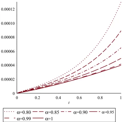
Fig. 2 The approximate solutionsI(t)forN=15

Tables 5, 6 and 7 show the values of T(t), I(t) andV(t), forN =15, α =0.75, 0.80, 0.85, 0.90, 0.95, 0.98.

Table 5. The values ofT(t)forN =15

t α =0.75 α=0.80 α=0.85 α=0.90 α=0.95 α=0.98

0.0 0.1 0.1 0.1 0.1 0.1 0.1

0.2 0.3670560 0.3165184 0.2790315 0.2501158 0.2272514 0.2157344 0.4 0.9419131 0.7540629 0.6246844 0.5309877 0.4606339 0.4264249 0.6 2.2858520 1.7039759 1.3317891 1.0784967 0.8979687 0.8133480 0.8 5.4360892 3.7737946 2.7836259 2.1489168 1.8178109 1.5242915 1.0 12.784070 8.2742007 5.7619568 4.2409152 3.2590105 2.8300579

Table 6. The values ofI(t)forN=15

t α=0.75 α=0.80 α=0.85 α=0.90 α=0.95 α=0.98

0.0 0 0 0 0 0 0

0.2 1.2151979e-5 1.0315362e-5 8.9043994e-6 7.7692349e-6 6.8290042e-6 6.3363901e-6 0.4 2.8204527e-5 2.2989039e-5 1.9385818e-5 1.6753726e-5 1.4746964e-5 1.3753198e-5 0.6 5.5742298e-5 4.2343235e-5 3.3864401e-5 2.8164952e-5 2.4155672e-5 2.2294605e-5 0.8 1.0695931e-4 7.4433150e-5 5.5403434e-5 4.3464569e-5 3.5585428e-5 3.2111872e-5 1.0 2.0660978e-4 1.3048453e-4 8.9263409e-5 6.5030221e-5 4.9905893e-5 4.3511235e-5

Table 7. The values ofV(t)forN =15

t α =0.75 α=0.80 α=0.85 α=0.90 α=0.95 α=0.98

0.0 0.1 0.1 0.1 0.1 0.1 0.1

0.2 0.0496485 0.0518676 0.0542264 0.0567019 0.0592643 0.0608295 0.4 0.0335988 0.0342057 0.0349582 0.0358789 0.0369869 0.0377472 0.6 0.0251079 0.0246948 0.0243227 0.0240146 0.0237983 0.0237253 0.8 0.0199388 0.0189386 0.0179038 0.0168397 0.0157587 0.0151098 1.0 0.0165367 0.0151977 0.0137958 0.0123158 0.0107509 0.0097708

Conclusion

This paper proposed a model based on performance of HIV virus for in faction of CD4+T cells. We formulated the model as a fractional differential equations system. The model was solved by collocation and Müntz-Legendre polynomials. Since the real solution is unknown, we compare obtained results forα =1, with those published in the literature. Further, we show results for different values ofα. Our findings demonstrate that the proposed method has a high accuracy compared to other methods. Besides, the presented method is simple and can be applied for solving the fractional cases.

References

1. Arafa A. A. M., S. Z. Rida, M. Khalil (2013). The Effect of Anti-viral Drug Treatment of Human Immunodeficiency Virus Type 1 (HIV-1) Described by a Fractional Order Model, Applied Mathematical Modelling, 37(4), 2189-2196.

2. Asquith B., C. R. M. Bangham (2003). The Dynamics of T-cell Fratricide: Application of a Robust Approach to Mathematical Modeling in Immunology, Journal of Theoretical Biology, 222(1), 53-69.

4. Chen Y., X. Ke, Y. Wei (2015). Numerical Algorithm to Solve System of Nonlinear Frac-tional Differential Equations Based on Wavelets Method and the Error Analysis, Applied Mathematics and Computation, 251, 475-488.

5. Chorukova E., I. Simeonov (2015). A Simple Mathematical Model of the Anaerobic Di-gestion of Wasted Fruits and Vegetables in Mesophilic Conditions, International Journal Bioautomation, 19, S69-S80.

6. Debnath L. (2003). Recent Applications of Fractional Calculus to Science and Engineer-ing, International Journal of Mathematics and Mathematical Sciences, 2003(54), 3413-3442.

7. Edwards J. T., N. J. Ford, A. C. Simpson (2002). The Numerical Solution of Linear Multi-term Fractional Differential Equations: Systems of Equations, Journal of Computational and Applied Mathematics, 148(2), 401-418.

8. Erturk V. S., Z. M. Odibat, S. Momani (2011). An Approximate Solution of a Fractional Order Differential Equation Model of Human T-cell Lymphotropic Virus I (HTLV-I) In-fection of CD4+T-cells, Computers and Mathematics with Applications, 62(3), 966-1002. 9. Esmaeili S., M. Shamsi, Y. Luchko (2011). Numerical Solution of Fractional Differen-tial Equations with a Collocation Method Based on Müntz Polynomials, Computers and Mathematics with Applications, 62(3), 918-929.

10. Ghasemi M., M. Tavassoli Kajani (2011). Numerical Solution of Time-varying Delay Sys-tems by Chebyshev Wavelets, Appllied Mathematics and Modelling, 35, 5235-5244. 11. Jafari H., V. Daftardar-Gejji (2006). Solving a System of Nonlinear Fractional Differential

Equations Using Adomian Decomposition, Journal of Computational and Applied Math-ematics, 196(2), 644-651.

12. Kumar N. V., L. Mathew, E. G. Wesely (2014). Computational Modelling of Pisum

sativumL. Superoxide Dismutase and Prediction of Mutational Variations throughin sil-icoMethods, International Journal Bioautomation, 18(2) 75-88.

13. Liu S., G. Wang, L. Zhang (2013). Existence Results for a Coupled System of Nonlinear Neutral Fractional Differential Equations, Applied Mathematics Letters, 26(12), 1120-1124.

14. Luchko Y., M. Rivero, J. J. Trujillo, M. P. Velasco, (2010). Fractional Models, Non-locality, and Complex Systems, Computers and Mathematics with Applications, 59(3), 1048-1056.

15. Maleki M., M. Tavassoli Kajani (2015). Numerical Approximations for Volterra’s Popu-lation Growth Model with Fractional Order via a Multi-Domain Pseudospectral Method, Applied Mathematical Modelling, 39, 4300-4308.

16. Merdan M., A. Gokdogan, A. Yildirim, (2011). On the Numerical Solution of the Model for HIV Infection of CD4+T Cells, Computers and Mathematics with Applications, 62(1), 118-123.

17. Milovanovic G. V. (1999). Müntz Orthogonal Polynomials and Their Numerical Evalua-tion, In: Applications and Computation of Orthogonal Polynomials, International Series in Numerical Mathematics, 13, 179-194.

18. Momani S., K. Al-Khaled (2005). Numerical Solutions for Systems of Fractional Differ-ential Equations by the Decomposition Method, Applied Mathematics and Computations, 162(3), 1351-1365.

19. Nowak M., R. May (1991). Mathematical Biology of HIV Infections: Antigenic Variation and Diversity Threshold, Mathematical Biosciences, 106(1), 1-21.

21. Perelson A. S., D. E. Kirschner, R. D. Boer, (1993). Dynamics of HIV Infection CD4+T Cells, Mathematical Biosciences, 114(1), 81-125.

22. Rossikhin Y. A., M. V. Shitikova (1997). Applications of Fractional Calculus to Dynamic Problems of Linear and Nonlinear Hereditary Mechanics of Solids, Applied Mechanics Reviews, 50(1), 15-67.

23. Srivastava V. K., M. K. Awasthi, S. Kumar (2014). Numerical Approximation for HIV Infection of CD4+T Cells Mathematical Model, Ain Shams Engineering Journal, 5(2), 625-629.

24. Tavassoli Kajani M., M. Maleki, A. Kilicman (2013). A Multiple-step Legendre-Gauss Collocation Method for Solving Volterra’s Population Growth Model, Math. Prob. Eng. 2013, 1-6.

25. Tavassoli Kajani M., S. Vahdati, Z. Abbas, M. Maleki (2012). Application of Rational Second Kind Chebyshev Functions for System of Integro-differential Equations on Semi-Infinite Intervals, Journal of Applied Mathematics, 2012, 1-11.

26. Tavassoli Kajani M., M. Maleki, M. Allame (2014). A Numerical Solution of Falkner-Skan Equation via a Shifted Chebyshev Collocation Method, AIP Conf Proc, 1629, 381-386.

27. Wang L., M. Y. Li (2006). Mathematical Analysis of the Global Dynamics of a Model for HIV Infection of CD4+T Cells, Mathematical Biosciences. 200(1), 44-57.

28. Yuzbasi S. (2012). A numerical approach to solve the model for HIV infection of CD4+T cells, Applied Mathematical Modelling, 36(12), 5876-5890.

29. Zhou W. G., Y. F. Cui, Y. Li (2015). A modified method combined with a support vector machine and Bayesian algorithms in biological information, International Journal Bioau-tomation, 19(2), 135-146.

Mojtaba Rasouli Gandomani, M.Sc.

E-mail: mojtabamath@yahoo.com

He was born on May 13, 1986 in Isfahan, Iran. He received the B.Sc. degree in Applied Mathematics form the Islamic Azad University, Mo-barakeh Branch, Isfahan, Iran, in 2010 and a M.Sc. degree in Ap-plied Mathematics from Islamic Azad University, Isfahan (Khorasgan) Branch, Isfahan, Iran, in 2015.

Majid Tavassoli Kajani, Ph.D. E-mail: mtavassoli@khuisf.ac.ir