* Corresponding author Tel.: +1-701-231-8277; fax: +1-701-231-7195 E-mail: [email protected] (M. Hamidi)
© 2012 Growing Science Ltd. All rights reserved. doi: 10.5267/j.ijiec.2011.08.015
Contents lists available at GrowingScience
International Journal of Industrial Engineering Computations
homepage: www.GrowingScience.com/ijiec
Modeling a four-layer location-routing problem
Mohsen Hamidia*, Kambiz Farahmanda, and Seyed Reza Sajjadib
a
Department of Industrial and Manufacturing Engineering, North Dakota State University, Dept. 2485, PO Box 6050, Fargo, ND 58108-6050, USA bTransSolutions, LLC., 14600 Trinity Blvd., Suite 200, Fort Worth, TX 76155, USA
A R T I C L E I N F O A B S T R A C T
Article history: Received 1 August 2011 Available online 10 August 2011
Distribution is an indispensable component of logistics and supply chain management. Location-Routing Problem (LRP) is an NP-hard problem that simultaneously takes into consideration location, allocation, and vehicle routing decisions to design an optimal distribution network. Multi-layer and multi-product LRP is even more complex as it deals with the decisions at multiple layers of a distribution network where multiple products are transported within and between layers of the network. This paper focuses on modeling a complicated four-layer and multi-product LRP which has not been tackled yet. The distribution network consists of plants, central depots, regional depots, and customers. In this study, the structure, assumptions, and limitations of the distribution network are defined and the mathematical optimization programming model that can be used to obtain the optimal solution is developed. Presented by a mixed-integer programming model, the LRP considers the location problem at two layers, the allocation problem at three layers, the vehicle routing problem at three layers, and a transshipment problem. The mathematical model locates central and regional depots, allocates customers to plants, central depots, and regional depots, constructs tours from each plant or open depot to customers, and constructs transshipment paths from plants to depots and from depots to other depots. Considering realistic assumptions and limitations such as producing multiple products, limited production capacity, limited depot and vehicle capacity, and limited traveling distances enables the user to capture the real world situations.
© 2012 Growing Science Ltd. All rights reserved Keywords:
Location-routing problem (LRP) Mixed-integer programming
1. Introduction
44
or several depots must be determined for a number of geographically dispersed cities or customers (The VRP Web, 2010). The objective of the VRP is to deliver a set of customers with known demands on minimum-cost vehicle routes originating and terminating at a depot (The VRP Web, 2010). The LRP solves the joint problem of determining the optimal number, capacity, and location of facilities serving more than one customer, and finding the optimal set of vehicle schedules and routes (Min et al., 1998). The common objective for LRPs is that of overall cost minimization, where costs can be divided into depot costs and vehicle costs (Nagy & Salhi, 2007). Its major aim is to capitalize on distribution efficiency resulting from a series of coordinated, non-fragmented movements and transfer of goods (Min et al., 1998). The main difference between the LRP and the classical location-allocation problem is that once the facility is located, the former requires customer visitation through tours, whereas the latter assumes the straight-line or radial trip from the facility to the customer (Min et al., 1998). LRPs are often described as a combination of three distinct components: (i) facility location, (ii) allocation of customers to facilities, and (iii) vehicle routing (Laporte, 1988). These three sub-problems are closely interrelated and cannot be optimized separately without running the risk of arriving at a suboptimal solution (Laporte, 1988).
From a practical viewpoint, location-routing forms part of distribution management (Nagy & Salhi, 2007). The LRP models can be applied in a variety of businesses and industries. Some of the applications mentioned in (Nagy & Salhi, 2007) are food and drink distribution, newspaper distribution, parcel delivery, and waste collection. Although most of the LRP models focus on distribution of consumer goods or parcels, there are also some applications in healthcare (e.g. blood bank location), military (e.g. military equipment location), and communications (e.g. telecommunication network design) (Nagy & Salhi, 2007). Operational research is all too often applied only in the affluent countries of Western Europe and North America, thus it is pleasing to see that LRP has also been applied in developing countries (Nagy & Salhi, 2007).
In some LRPs, e.g. a drink distribution system, customers are wholesalers or retailers and in some, e.g. a mail delivery system, customers are the final customers. From a mathematical point of view, LRP can usually be modeled as a combinatorial optimization problem (Nagy & Salhi, 2007). LRP is an NP-hard, Non-deterministic Polynomial-time hard, problem, as it encompasses two NP-hard problems of facility location and vehicle routing (Nagy & Salhi, 2007). Balakrishnan et al. (1987), Laporte (1988), Min et al. (1998), and Nagy and Salhi (2007) have surveyed the LRP models. In this section, the LRP models are classified according to the number of layers in the distribution network. Two-Layer LRPs: Most of the LRP models proposed in the literature are related to a simple distribution network with two layers of depots and customers (Ambrosino and Scutella, 2005).
In these models, three problems are to be solved: 1) location problem: given a set of candidate sites, how many depots are needed and where should they be located?, 2) allocation problem: which customers should be allocated to which depot?, and 3) routing problem: how many tours should exist for each depot, which customers should be on each tour, and what is the best sequence of the customers on each tour?. Many studies have been performed on two-layer LRPs of which some are reviewed in this section.
Perl and Daskin (1985) presented a heuristic method to solve a two-layer LRP with capacitated depots and vehicles. They decomposed the LRP into three sub-problems of mutli-depot vehicle-dispatch problem, warehouse location-allocation problem, and multi-depot routing-allocation problem. Then, they solved the sub-problems in a sequential and iterative manner while accounting for the dependency between them. Heuristic methods were developed to solve the first and third sub-problems, and an exact method was applied to solve the second sub-problem.
solved all of the three sub-problems introduced by Perl and Daskin (1985) heuristically in an iterative manner and improved the solutions.
Tuzun and Burke (1999) presented a two-phase tabu search algorithm that iterates between location and routing phases in order to search for better solutions of a two-layer LRP with capacitated vehicles.
Wu et al. (2002) presented a decomposition-based method for solving a two-layer LRP with multiple fleet types and a limited number of vehicles for each different vehicle type. The problem is decomposed into two sub-problems (the location-allocation problem, and the vehicle routing problem) and then each sub-problem is solved in a sequential and iterative manner by a combined simulated annealing and tabu search framework.
Prins et al. (2007) presented a lagrangean relaxation-granular tabu search heuristic to solve a two-layer LRP with capacitated depots and vehicles. In each iteration, the algorithm performs a solution for one location phase and one routing phase. The location phase is solved by a lagrangean relaxation of the assignment constraints, and the routing phase is solved using a granular tabu search heuristic. The algorithm also tries to further improve the solution by performing a local search phase.
Duhamel et al. (2010) proposed a heuristic for solving a two-layer LRP with capacitated depots and vehicles. The heuristic is a greedy randomized adaptive search procedure (GRASP) hybridized with an evolutionary local search (ELS). The method builds giant tours and then split them into feasible routes by using a splitting procedure.
Yu et al. (2010) proposed a simulated annealing based heuristic (SALRP) for solving a two-layer LRP with capacitated depots and vehicles. The heuristic features a special solution encoding scheme that integrates location and routing decisions in order to enlarge the search space so that better solutions can be found.
Three-Layer LRPs: Few studies have been performed on three-layer LRPs. Three-layer LRP models usually consist of three layers of plants, depots, and customers. In these models, plants are fixed and their locations are known. The location problem is the problem of locating depots. The allocation and routing problems and decisions depend on the structure of the network and differ from one model to another.
Jacobsen and Madsen (1980) and Madsen (1983) presented three heuristics to solve a three-layer LRP to design a newspaper distribution network. The network consists of one printing office, transit points, and sales points. In the network, newspapers are delivered from the printing office to transfer points and from there to sales points. The problem includes one location problem, location of transit points; one allocation problem, allocating sales points to transfer points; two routing problems, primary tours from the printing office to transfer points and secondary tours from transfer points to sales points; and one problem of sequencing primary tours.
Perl and Daskin (1985) formulated a three-layer LRP with plants, warehouses, and customersbut as mentioned previously presented a heuristic method to solve a two-layer LRP with warehouses and customers. The formulation includes location of warehouses, allocation of customers to warehouses, routing from warehouses to customers, and transportation from plants to warehouses.
Bookbinder and Reece (1988) formulated a three-layer LRP. The distribution network consists of plants, depots, and customers. Multi-type products are shipped from plants to depots and then from depots to customers. The problems considered are location of depots, allocation of customers to depots, routing from depots to customers, and transportation from plants to depots. They decomposed the problem into three sub-problems (location-allocation problem, routing problem, and transportation problem) and presented a solution procedure that solves the sub-problems sequentially in an iterative manner.
46
first-level routing, and 4) the second-level routing between DC’s and other clients not included in the first-level routing. To solve the problem, they developed a hybrid genetic algorithm embedded with a routing heuristic.
Four-Layer LRPs: Only few studies have been performed on four-layer LRPs. These studies are as follows.
Ambrosino and Scutella (2005) formulated a four-layer LRP with one plant, central depots (CD), transit points (TP), and customers. The plant sends goods (one type of product) to CDs. CDs transfer them to TPs and they may serve big customers. And TPs deliver goods to customers. The problems considered are: 1) location at two levels, locating CDs and TPs, 2) allocation at two levels, allocating TPs and customers to CDs and allocating customers to TPs, 3) routing at two levels, routing between CDs, TPs, and customers starting from CDs and routing between TPs and customers starting from TPs, 4) the quantity of good which must be shipped from the plant to CDs and from CDs to TPs.
Lee et al. (2010) formulated a four-layer LRP which includes suppliers, manufacturers, distribution centers (DC), and customers. The study considers a supply chain in which suppliers send materials to manufacturers, manufacturers send products to DCs, and DCs send products to customers. The problems considered are: 1) location at two layers, locating manufacturers and DCs, 2) allocation at two layers, allocating suppliers to manufacturers and allocating customers to DCs, 3) routing at two layers, routing between manufacturers and suppliers starting from manufacturers and routing between DCs and customers starting from DCs, and 4) transportation problem, transporting products from manufacturers to DCs. They presented a mixed integer programming model that considers a single item (product) and capacity limitation for suppliers, manufacturers, and DCs. They developed a heuristic algorithm based on LP-relaxation (relaxed binary variables) to solve the problem.
2. Problem definition
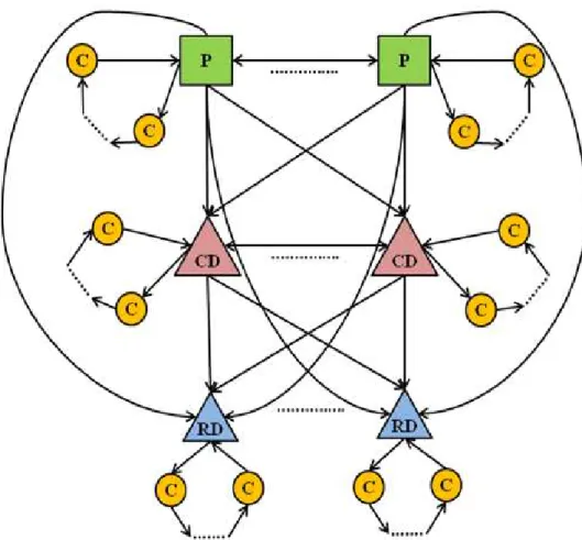
As one of the suggestions for future research mentioned by Nagy and Salhi (2007), the most recent survey on LRP, one of the gaps in the LRP literature is modeling and solving complex situations. The problem under consideration in this paper is a four-layer LRP. The general characteristics of the network are as follows. To visualize the four-layer LRP, the graphic of the network is presented in Fig. 1.
1) The network consists of plants (P), layer 1 (in green); central depots (CD), layer 2 (in purple); regional depots (RD), layer 3 (in blue); and customers (C), layer 4 (in orange).
2) Plants produce multiple-type products.
3) Products can be shipped from plants to other plants, CDs, RDs, or customers. From CDs, products can be shipped to other CDs, RDs, or customers. And from RDs, products are delivered to customers. Basically, customers’ demands can be satisfied directly by plants, CDs, or RDs.
4) Each route between facilities (plants, CDs, and RDs) consists of only two facilities (tours are not allowed). To deliver products to customers, multiple customers can be visited in one route (tours are allowed). Also, multiple tours are allowed from each facility to deliver products to different groups of customers to be allocated to the facility. To avoid complexity in the figure, one tour is shown from each facility to customers but as mentioned above, multiple tours are allowed. 5) Products can be shipped within layer 1 from one plant to another plant since some products may
points while RDs are not. Besides delivering products to customers, CDs mix different products obtained from plants and prepare and ship the requirements of other depots, especially RDs.
Fig. 1. The graphic of the four-layer LRP
Basically, the presented LRP is a combination of location, allocation, vehicle routing, and transshipment problems. A transshipment problem allows shipment between supply points and between demand points, and it may also contain transshipment points through which goods may be shipped on their way from a supply point to a demand point (Winston, 2003). The problems to be solved and the decisions to be made in this LRP are as follows:
1) Location problem at two layers (locating CDs and RDs)
• Given a set of candidate sites for CDs, how many CDs are needed and where should they be located?
• Given a set of candidate sites for RDs, how many RDs are needed and where should they be located?
2) Allocation problem at three layers (assigning customers to plants, CDs, and RDs)
• Which customers should be served by each plant?
• Which customers should be served by each CD?
• Which customers should be served by each RD? 3) Transshipment problem
• In each plant how many units of each product should be produced?
48
• From each CD how many units of each product should be directly shipped to which CD or RD?
4) Vehicle routing problem at three layers (tours from plants, CDs, and RDs to customers)
• To visit and serve the customers allocated to a plant, a CD, or an RD, what sequence of customers is the best (what is the minimum-cost tour)?
The main assumptions and limitations of the model are as follows:
1) Plants are fixed, and their locations are known.
2) CDs and RDs are to be located in a set of candidate locations. 3) Customers’ locations are known, and their demands are known. 4) Plants have limited production capacity for producing products. 5) CDs and RDs have limited space capacity.
6) Vehicles have limited capacity, and one type of vehicle is used to deliver products to customers. 7) Each customer’s demand is less than the vehicle’s capacity (less than truck load (LTL)).
8) The customer’s demand is satisfied by only one vehicle (there will be only one tour for each customer).
9) Each tour starts and ends at the same facility.
10)Limitations on travel distances are considered. In delivering products to customers, lengths of tours are limited. Some reasons for considering this limitation are perishable items being transported, limited drivers’ service hours per day/tour, and faster and more reliable delivery to customers. Also shipments between two facilities (plants, CDs, or RDs) cannot take place if the distance between the facilities is more than a maximum allowable distance.
3. Mathematical model
To solve the four-layer LRP and make the decisions mentioned in the previous section, the following mixed integer programming model is developed. The components of the model are as follows:
Sets:
P : set of plants
CD : set of candidate sites for CDs
RD : set of candidate sites for RDs
C : set of customers
T : set of tours
PR : set of products
Input parameters:
oj : cost of operating a depot at site j
scm : cost per mile of direct shipment of one unit of product m between facilities (plants, CDs, and RDs)
tdgh : travelling distance between point g and point h
tc : travelling cost per mile of a vehicle on a tour
ft : fixed cost of a tour
dim : demand of customer i for product m
sum : number of standard units per one unit of product m in terms of space needed
vc : vehicle capacity, number of standard units
dcj : capacity of depot (CD, or RD) j, number of standard units
pcpm : production capacity of plant p for product m
fd : maximum allowable distance to be travelled for direct shipment from one facility to another facility
Decision variables:
Xghk = 1 if point g immediately precedes point h on tour k and 0 otherwise
Yij = 1 if customer i is served by facility j and 0 otherwise
Zj = 1 if a depot is located at site j and 0 otherwise
Ujlm : Number of units of product m to be shipped from facility j to facility l
Vpm : Number of units of product m to be produced in plant p
Formulation: Minimize
∑∑ ∑
∑ ∑
∑
∑ ∑
∑
∑
∈ ∈ ∈ ∪ ∪ ∈ ∈ ∪ ∪ ∪ ∈ ∪ ∪ ∪ ∈ ∈ ∪ ∪ ∈ ∪ ∪ ∈ + + + Tk h Cg P CD RD ghk
T
k h P CD RD Cg P CD RD C
ghk gh PR
m l P CD RDj P CD
jlm jl m RD CD j j j X ft X td tc U td sc Z o ) ( ) ( (1) subject to
∑ ∑
∈ ∈ ∪ ∪ ∪ = Tk h P CD RD C ihk
X 1, ∀i∈C (2)
∑
∑
∪ ∪ ∪ ∈ ∈ ∪ ∪ ∪ = − C RD CD Pg g P CD RD C
hgk
ghk X
X 0, ∀h∈P∪CD∪RD∪C, ∀k∈T (3)
{ }
∑
∑
∑
∈ ∈ ∪ ∪ ∪ − ∈
≥ T
k h P CD RD C Sg S ghk
X 1,
∀S ⊂P∪CD∪RD∪C, P∪CD∪RD⊆S (4)
∑ ∑
∪ ∪ ∈ ∈ ≤ RD CD Pj i C
ijk
X 1, ∀k∈T (5)
∑
∑
∪ ∪ ∪ ∈ ∈ ∪ ∪ ∪ ≤ − + C RD CD P h ij C RD CD P h jhkihk X Y
X 1 , ∀i∈C, ∀j∈P∪CD∪RD, ∀k∈T (6)
∑
∑
∪ ∪ ∪ ∈ ∈ ∪ ∪ ∪ ≤ C RD CD Ph g P CD RD C ghk ghX tl
td , ∀k∈T (7)
vc X su d PR
m h P CD RD Ci C
ihk m
im ≤
∑
∑ ∑
∈ ∈ ∪ ∪ ∪ ∈
, ∀k∈T (8)
∑
∑
∑
∈ ∈ ∪ ∪ ∈ − + = P l lpm C i ip im RD CD P l plmpm U d Y U
50 1 =
∑
∪ ∪ ∈P CD RD jij
Y , ∀i∈C (10)
pm pm pc
V ≤ , ∀p∈P, ∀m∈PR (11)
0 = − −
∑
∑
∑
∪ ∈ ∈ ∪∈ lCD RD
jlm C i ij im CD P l
ljm d Y U
U , ∀j∈CD, ∀m∈PR (12)
0 = −
∑
∑
∈ ∪ ∪∈ iC
ij im RD CD P l
ljm d Y U
, ∀j∈RD, ∀m∈PR
(13) 0 ≤ − +
∑
∑ ∑
∪ ∈∈ ∈ l CD RD j j
jlm PR
m iC
ij m
imsu Y U dc Z
d , ∀j∈CD (14)
0
≤ −
∑ ∑
∈PR ∈ j j
m iC
ij m
imsu Y dc Z
d , ∀j∈RD (15)
0 )
( ≤
− jlm
jlm
jlU fd U
td , ∀j∈P∪CD, ∀l∈P∪CD∪RD, ∀m∈PR (16)
{ }
0,1∈
ghk
X , ∀g,h∈P∪CD∪RD∪C, ∀k∈T (17)
{ }
0,1∈
ij
Y , ∀i∈C, ∀j∈P∪CD∪RD (18)
{ }
0,1∈
j
Z , ∀j∈P∪CD∪RD (19)
0
≥
jlm
U , ∀j,l∈P∪CD∪RD, ∀m∈PR (20)
0
≥
pm
V , ∀p∈P, ∀m∈PR (21)
The objective function is the distribution cost including depot cost, shipment (between facilities) cost, and delivery (to customers) cost (fixed and variable costs of tours). Constraints (2) ensure that each customer is on only one tour (is served by only one vehicle). Constraints (3) are the tour continuity constraints which imply that every point that is entered by a vehicle should be left by the same vehicle. Constraints (4) require that every tour be connected to a facility; they ensure that there is at least one connection from the set of facilities and any customer(s) to the rest of the customers. Constraints (5) state that each tour cannot be operated from multiple facilities. Constraints (6) link the allocation and routing problems; they specify that a customer can be allocated to a facility only if there is a tour from that facility going through that customer. Constraints (7) limit the length of each tour. Constraints (8) guarantee that the space needed for the demand of customers in each delivery does not exceed the capacity of a vehicle. Constraints (9) calculate the number of each product that has to be produced in each plant. Constraints (10) assure that each customer is assigned to only one facility; although this set of constraints is not seen in LRP models, during modeling and solving some problems it was seen that because of having constraints (9) in this particular LRP, it is necessary to have this set of constraints. Constraints (11) state that the number of products to be produced in each plant cannot exceed the production capacity of the plant. Constraints (12) and (13) specify that the flow into a depot is equal to the flow out of the depot. Constraints (14) and (15) state that the space needed for a depot should not exceed the depot’s capacity. These constraints also assure that a depot cannot be opened unless it is used for delivering products to customers or transshipping products to other depots. Constraints (16) guarantee that a direct shipment between two facilities takes place only if the distance between the facilities is less than a maximum allowable distance. Constraints (17), (18), and (19) are binary integer constraints and constraints (20) and (21) are non-negativity constraints for decision variables.
4. An Illustrative example
(p T th T T D T C D T 5 L al m d n p p co C p u o R A
points 5 and The optimal n
he decision v
Table 1
The optimal s Decision / Va
our routing Customer allo Depot locatio
ransshipmen
. Conclusion
LRP is an N llocation, an multi-product istribution n etwork. In th roduct distr rogramming onstructs tou Considering
roduction ca ser to captur f time, a hyb
References
Ambrosino, D models. E
d 6), and fou network and variables are
solution ariable
(Xghk) ocation (Yij) on (Zj)
nt (Vpm and U
n
NP-hard pro nd vehicle ro
t LRP is ev network wh his paper, a ribution netw g model. Th
urs from fac realistic as apacity, limi re the real w brid GRASP
D., & Scute European Jo
ur customers d solution ar e presented.
Ujlm)
oblem which outing decis ven more co here multipl
new comple work is pro he mathema cilities to cu sumptions a ited depot a world situatio P-tabu search
lla, M. G. (2 ournal of Op
(points 7, 8 re shown in F
Fig. 2. The o
X6(10)1 = Y75 = Y8 Z4 = Z5 = V11 = 40 U451 = 4
h is used t sions to desi omplex as i e products ex four-layer oposed. The atical mode ustomers, an and limitati and vehicle c
ons. In order h metaheuris
2005). Distr perational R
8, 9, and 10) Fig. 2 and T
optimal netw
= X(10)91 = X96
85 = 1 ; Y96 = = Z6 = 1 0, V12 = 15 ; 40, U452 = 15
to simultane ign an optim it deals wit
are transpo r LRP mode e four-layer l locates de nd constructs ons such a capacity, an r to solve lar stic is under
ribution netw esearch, 165
and two typ Table 1. In T
work
Variable
61 = 1 ; X572 Y(10)6 = 1
V21 = 50, V2 5 ; U261 = 50
eously take mal distributi th the decis orted within
el that repres LRP is pr epots, alloc s transshipm
s producing d limited tra rge-size prob developmen
work design 5(3), 610-62
pes of produ Table 1, the o
Values
= X782 = X85
22 = 25 ; U141 , U262 = 25
into consid ion network
ions at mul and betwe sents a multi resented by
ates custom ment paths b g multiple p
aveling dista blems in a re nt.
n: New prob 24.
ucts are prod optimal valu
52 = 1
1 = 40, U142 =
deration loc k. Multi-laye ltiple layers een layers o
i-layer and m a mixed-in mers to faci
between faci products, lim ances enable easonable am
52
Balakrishnan, A., Ward, J. E., Wong, R. T. (1987). Integrated facility location and vehicle routing models: Recent work and future prospects. American Journal of Mathematical and Management Sciences, 7(1&2), 35–61.
Bookbinder, J. H., & Reece, K. E. (1988). Vehicle routing considerations in distribution system design. European Journal of Operational Research, 37, 204-213.
Duhamel, C., Lacomme, P., Prins, C., & Prodhon, C. (2010). A GRASP×ELS approach for the capacitated location-routing problem. Computers & Operations Research,37(11), 1912-1923. Hansen, P. H., Hegedahl, B., Hjortkjaer, S., & Obel, B. (1994). A heuristic solution to the warehouse
location-routing problem. European Journal of Operational Research, 76(1), 111-127.
Jacobsen, S. K., & Madsen, O. B. G. (1980). A Comparative Study of Heuristics for a Two-Level Routing-Location Problem. European Journal of Operational Research, 5(6), 378-387.
Laporte, G. (1988). Location-routing problems. In: Golden, B. L., & Assad, A. A. (Editors), Vehicle Routing: Methods and Studies, North-Holland, Amsterdam. 163–198.
Lee, J., Moon, I., & Park, J. (2010). Multi-level supply chain network design with routing. International Journal of Production Research, 48(13), 3957-3976.
Lin, J., & Lei, H. (2009). Distribution systems design with two-level routing considerations. Annals of Operations Research, 172(1), 329-347.
Madsen, O. B. G. (1983). Methods for solving combined two level location routing problems of realistic dimensions. European Journal of Operational Research, 12, 295-301.
Min, H., Jayaraman, V., & Srivastava, R. (1998). Combined location-routing problems: A synthesis and future research directions. European Journal of Operational Research, 108(1), 1-15.
Nagy, G., & Salhi S. (2007). Location-routing: Issues, models and methods. European Journal of Operational Research, 177(2), 649-672.
Perl, J., & Daskin, M. S. (1985). A warehouse location-routing problem. Transportation Research B, 19B(5), 381-396.
Prins, C., Prodhon, C., Ruiz, A., Soriano, P., & Calvo, R. (2007). Solving the Capacitated Location-Routing Problem by a Cooperative Lagrangean Relaxation-Granular Tabu Search Heuristic. Transportation Science, 41(4), 470-483.
The VRP Web. http://neo.lcc.uma.es/radi-aeb/WebVRP/index.html. Retrieved April 24, 2010.
Tuzun, D., & Burke, L. I. (1999). A two-phase tabu search approach to the location routing problem. European Journal of Operational Research, 116(1), 87-99.
Winston, W. L. (2003). Operations Research: Applications and Algorithms (4th edition). Duxbury Press.
Wu, T., Low, C., & Bai, J. (2002). Heuristic solutions to multi-depot location-routing problems. Computers and Operations Research, 29(10), 1393–1415.
Yu, V. F., Lin, S., Lee, W., & Ting, C. (2010). A simulated annealing heuristic for the capacitated location routing problem. Computers & Industrial Engineering, 58(2), 288-299.