APPROXIMATION OF VOLUME AND BRANCH SIZE DISTRIBUTION OF TREES
FROM LASER SCANNER DATA
Pasi Raumonen (1), Sanna Kaasalainen (2), Mikko Kaasalainen (1), and Harri Kaartinen (2)
(1) Department of Mathematics, Tampere University of Technology P.O. Box 553, FI-33101 Tampere, Finland, [email protected] (2) Remote Sensing and Photogrammetry, Finnish Geodetic Institute
P.O.Box 15, FI-02431 Masala, Finland
KEY WORDS: LIDAR, point cloud, trees, classification, size approximation, carbon cycle
ABSTRACT:
This paper presents an approach for automatically approximating the above-ground volume and branch size distribution of trees from dense terrestrial laser scanner produced point clouds. The approach is based on the assumption that the point cloud is a sample of a surface in 3D space and the surface is locally like a cylinder. The point cloud is covered with small neighborhoods which conform to the surface. Then the neighborhoods are characterized geometrically and these characterizations are used to classify the points into trunk, branch, and other points. Finally, proper subsets are determined for cylinder fitting using geometric characterizations of the subsets.
1 INTRODUCTION
The total above-ground volume, the branch size distribution, and other size and shape parameters of trees are of economic and sci-entific interests. For example, carbon cycle estimations of forests require the branch size distribution of trees for the accurate de-termination of branch decay times (carbon release as a function of time). One way to approximate these parameters is to use dense terrestrial laser scanner produced point clouds (Pfeifer et al., 2004; Maas et al., 2008; Rutzinger et al., 2010). In many of these methods, the point cloud is mapped to a voxel space, where it is segmented into branches by, e.g., mathematical morphology (Gorte and Pfeifer, 2004). Then cylinders are fitted into each branch to approximate the size. Furthermore, the shape and size of the tree cross-sections can be more accurately analyzed using, e.g., free-form curves (Pfeifer and Winterhalder, 2004).
In this paper we propose a new method for automatically approx-imating the size parameters and structures of trees from point clouds. The basic assumptions of the method are that the point cloud is a sample of a surface in the 3D-space and the surface, i.e. the tree, can be locally approximated with cylinders. Other a pri-ori assumptions about the data and structure of trees are used as well. The basis of the method is a local approach where the point cloud is covered with small neighborhoods which conform to the surface. Then these neighborhoods are geometrically character-ized and, based on these characterizations, the neighborhoods are classified into trunk, branch, and other points. Finally, cylinders are fitted to proper subsets to approximate the size. Notice that voxel spaces are not used, although partitions of the point cloud into cubical cells are used to produce the coverings quickly.
2 OBTAINING THE POINT CLOUDS
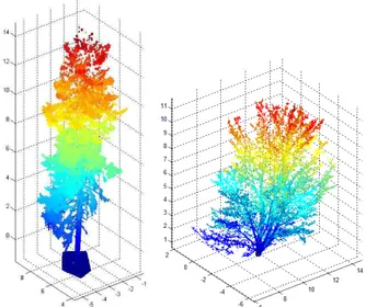
In this paper we used two point cloud samples, one from a conif-erous tree and the other from a broadleaf tree without leafs (see Fig. 1). The trees were scanned from three different directions to have a comprehensive cover of the branching structure. The scans were registered to a common coordinate system via spher-ical reference targets placed in the measured area. The measured point clouds for both trees have about 1.7 million points.
The coniferous tree was scanned with a Faro Photon120 and the broadleaf tree with a Leica HDS6100 terrestrial laser scanner.
Figure 1: Point clouds from a coniferous (left) and a deciduous tree (right).
Both scanners use phase modulation with different carrier wave-lengths for the distance measurement. The distance measurement accuracy is 2-3 mm at 25 m. Scanner specifications are given in Table 1.
Faro Photon Leica HDS6100
Wavelength 785 nm 650-690 nm
Unambiguity range 153 m 79 m
Field-of-view 360◦×320◦ 360◦×310◦
Beam diameter 3.3 mm 3 mm
Beam divergence 0.16 mrad 0.22 mrad
Table 1: Scanner specification.
3 LOCAL APPROACH
The laser-scanner produced point cloudPM from a tree is
as-sumed to be a sample of a surfaceMembedded in the Euclidean spaceR3
. The point cloudPM inherits distances (metric) and
i.e. when the distances measured along the surfaceMare small, they are nearly equal to the distances of the embedding space which are measured ‘directly through the tree and air’. Further-more, the structure and size of trees can be locally reasonably ap-proximated with cylinders. This suggests that although the global detailed structure of the surfaceMis complex and unknown, the local structure can be analyzed much more easily from the point cloud samplePM. We propose the following local approach to
the automatic size approximation:
1) Cover: The point cloud is covered with small neighborhoods. 2) Characterization: The neighborhoods are characterized geo-metrically.
3) Classification: Based on the characterizations the neighbor-hoods are classified to be part of trunk, branches, or other points. 4) Local size approximation: Determine proper subsets and fit cylinders to approximate the size.
5) Global characteristics: From local size data determine global characteristics such as the total volume and branch size distribu-tion.
The details of these steps require approximations of the struc-tures, such as metric and topology, of the surfaceM from the point cloudPM. Next we give details on the approximation of
some needed structures ofM.
4 APPROXIMATION OF STRUCTURES
The point cloudPM ⊂ R3 inherits the distance function dP
from the Euclidean embedding spaceR3 as a restriction of the Euclidean metricdofR3
; i.e. dP(p, q) = d(p, q)holds for all p, q ∈ PM. Similarly, the neighborhoods ofPM are defined as
restrictions of the neighborhoods ofR3intoPM. A particularly
important class of neighborhoods ofPM consists of ther-balls B(p, r) ={q∈PM|dP(p, q)< r}(these are sometimes called
fixed distance neighborhoods). Notice that these structures are globally defined for the point cloud, but they need not be good approximations of the corresponding global structures of the sur-faceM. For example, the intrinsic metricdMofM, which
mea-sures along the surface, gives always equal or greater distances thandP, i.e. the inequalitydP(p, q) ≤ dM(p, q)holds for all p, q∈PM. Particularly, for pointsp, q∈PMthat are in the tips
of different but nearby branches, the distances in terms of metrics
dP anddMsatisfydP(p, q)<< dM(p, q). However, locally the
inherited structures of the point cloud are good approximations: for pointsp, q ∈ PM which are close to each other in terms of
the intrinsic metricdM, the approximationdM(p, q)≈dP(p, q)
holds.
Next we show how connected components or connectedness of subsets of the surfaceM can be determined using a cover of
M withr-balls. Two points of PM are, by definition, in the
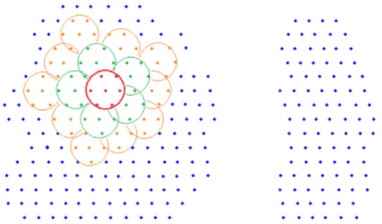
same component if there exists a chain of smallr-balls such that the consecutive balls are not disjoint (see Fig. 2). Notice that by this definition only those components ofM whose distance measured withdP is equal or larger thanrcan be recognized.
Thus, the radiusrof the balls should be so small that everyr -ball itself is connected in the sense that it corresponds to a con-nected set of the surfaceM: The corresponding set of ther-ball
B(p, r)⊂PM onM is defined to be the intersection ofM and
ther-ball of the embedding spaceR3
centered at pointp, i.e. the set{q ∈ M|d(p, q) < r}, wheredis the Euclidean metric of
R3. Now if we have a coveringCofPM with small connected r-balls and know inside which balls each point is, we can de-termine the connected components with the following algorithm (see Fig. 3):
1) Select any ballBofCwhich is not already assigned to some
Figure 2: Definition of connected components. The pointspand
qare in the same component because there is a chain of overlap-pingr-balls connecting them. Because there are no such chains between the pointsvandw, they are in different components.
Figure 3: Determination of connected components. An arbitrary ball (red) is chosen and it is expanded by an iterative process where overlapping balls are added to the existing ones.
component and assignA0=B.
2) Find all the balls B = {Bj} in the coveringC such that Bj∩Aiis not empty and assignAi+1=Ai∪B.
3) IfAi+16=Aiholds, repeat 2). IfAi+1 =Aiholds, thenAi
is a component and continue from 1.
Finally, we show how the tangent planes and surface normals of the surfaceM for points ofPM can be approximated using the
metric and neighborhoods defined above. In the approximation we fit planes to the neighborhoods using the total least squares method (Mitra et al., 2004). The solution of this problem is given by the eigenvectors of the scatter matrixCof the subsetB⊂PM
where the plane is fitted:
C(B) = Σm
i=1(xi−x¯)(xi−x¯)T, (1)
wherexi∈B,mis the number of points inB, andx¯=m1Σmi=1xi
is the mean of pointsxi. The unit eigenvectors corresponding to
the two largest eigenvalues ofCspan the tangent space and the unit eigenvector corresponding to the smallest eigenvalue is a sur-face normal.
With these approximated structures we can present details of our method outlined in the section 3. The first step in the method is to cover the point cloud with small sets.
5 COVER
We want to generate a coverC ={Bi}of the point cloudPM
withr-ballsBisuch that the center point of each ball is not
in-cluded to other balls. The radiusrshould be as large as possible such that the local metric approximationdM ≈ dP still holds
8.09 8.1 8.11 8.12 8.13 −0.6 −0.58 −0.56 −0.54 −0.52 −0.5 2.95 2.96 2.97 2.98 2.99 3 10.06 10.08 10.1 10.12 −1.3 −1.28 −1.26 −1.24 −1.22 −1.2 1.48 1.5 1.52 1.54 1.56 1.58 1.6
Figure 4: A subset B (red circles) is elongated (left) and this is reflected in the eigenvalues (λ1, λ2, λ) and eigenvectors
(u1, u2, u3) ofC(B)such thatλ1 >> λ2 ≥λ3 holds andu1
approximates the directionBis elongated. When the eigenval-uesλ1andλ2are approximately equal (right), there is no clear
direction of elongatedness.
choice of radiusr is about the size of the most branches. To generate the coverC quickly, we first partition the embedding spaceR3into cubical cells such that the side length of the cubes isr. This partition ofR3
also partitions the point cloudPMinto
cubical cells and the cells where each point belongs can be di-rectly calculated from the coordinates of the points. Now the ball
B(p, r)is contained in ther-cube containing the pointpand in its 26 neighboringr-cubes. To generate the cover, we take the first pointp1fromPMand calculate itsr-ball neighborhoodB(p1, r),
which is the first ball in the coverC. Then we take another point fromPM which is not yet specified into a ball and define itsr
-ball. This process is continued until all points are specified into balls. During this process we also determine the balls each point belongs in.
The coverCcan be used to generate another coverCL={Li}
ofPM with larger setsLithat are connected and conform to the
surfaceM: eachLiis the union of all the ballsBj ∈Cwhose
intersection withBiis not empty (For example, in the Fig. 3 the
setLicorresponding to the red ball is the red ball together with
the green balls). This process can be repeated to generate covers with even larger sets that are connected and conform toM.
6 CHARACTERIZATION
The second step in our local approach is the characterization of the cover setsBandL. The cover sets (and subsets ofPM in
general) are geometrically characterized using the scatter matrix
C(B). Assume that the points ofBare approximately uniformly distributed over part ofM. Furthermore, let{u1, u2, u3}be the
unit eigenvectors ofC(B)such that the corresponding eigenval-ues satisfyλ1 ≥ λ2 ≥ λ3. With these assumptions we now
define some characteristics.
The unit vectoru1approximates the direction in which the subset
Bis the most elongated (see Fig. 4). This gives our first char-acteristics, the directionD(B) = u1. On the other hand, how
elongated the subsetBis can be estimated by the ratio ofλ1and
λ2(see Fig. 4). Thus the second characteristics, the
elongated-nessE(B) =λ1
λ2. Similarly with the flatnessF(B) =
λ1
λ3 we can asses how planar the subsetBis.
The vectorsD(B)can be used, e.g,. to define the local direction of branches. Besides, because neighborhoods of same radius are usually more elongated for branch points than for trunk points, the valueE(B)is usually larger for branch points than for trunk points. Similarly the flatness values for ground points are usually larger than for trunk points, which in turn usually have larger
Figure 5: Classification of ground points. Left: The blue points denote the cover sets Li that are initially classified as ground
points (r= 0.03,fg= 100,pg= 0.5). Right: The final
classifi-cation of ground points.
flatness values than branch points. A very large value ofF(B) indicates thatBis nearly planar.
The trunk is often nearly straight and has generally a different direction than the branches and the ground. For point clouds this means that the part of the surfaceM corresponding to the trunk has a ‘characteristic’ direction in the embedding spaceR3given globally by a unit vectorV ∈R3
. Then setsBthat are parallel with the trunk direction have unit tangent vectors nearly parallel toV; i.e. the valuePV(B), defined as the maximum value of the
dot productV·v, wherevis a unit tangent vector ofB, is close to one. The characteristic direction vectorV of a trunk can be often be known a priori quite accurately or it can be approximated well with the vectorD(PM)(if the tree is taller than it is wide).
7 CLASSIFICATION
When the cover sets ofCandCLare geometrically
character-ized, the next step in our method is to use these characterizations to classify the sets as ground (other), trunk, and branch points. We give examples how to employ the characterizations together with a priori assumptions on data and the structure of the trees.
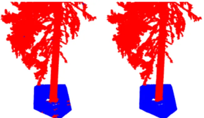
Often the ground points have the most planar neighborhoods in the point clouds, and they are not parallel to the trunk. Using this assumption we take a high flatness valuefgand small parallelism
valuepgand find the partG0 ={Li|F(Li)> fg &PV(Li)< pg}of the coverCL(see Fig. 5). Then we either take the mean
of pointsG0 or the largest connected component ofG0, which
is near the true ’ground level’. The mean ofG0 is a faster way
to approximate the ground level, but the largest connected com-ponent ofG0is more reliable. Then the ground pointsGcan be
defined as all those setsLiwhich are near the ground level and
are not parallel to the trunk, i.e.PV(Li)is small (see Fig. 5).
Next we give an example of the initial classification of the trunk points. They are those cover setsT0 = {Li}that are not
clas-sified as ground points and which are 1) parallel to the trunk di-rectionV, i.e. PV(Li) > pt holds, and 2) not elongated, i.e.
E(Li)< etholds, and 3) quite flat, i.e. F(Li)> ftholds. The
numberspt,et, andftshould be such that they will not exclude
any or only a few real trunk point but at the same time will ex-clude most of the real branch points. By trial and error we have determined suitable parameter values, see Fig. 6. The suitable parameter values depend particularly on the radiusrof the cover setsB. T0 will probably contain numerous branch points but
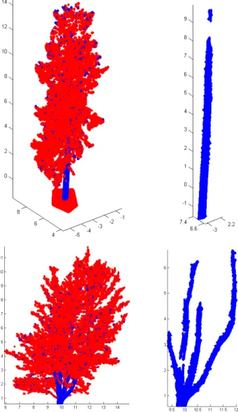
Figure 6: Classification of trunk points. Top: The blue points denote the cover sets that are initially classified as trunk points (r = 0.03, pt = 0.8,et = 3,ft = 15). Bottom: The final
classification of trunk points, where only the largest components (over 2000 points) of the initial classification are accepted.
by excluding those connected components ofT0that have a small
number of points (see Fig. 6). On the other hand, if the trunk is approximately straight, we can have an estimate of the trunk axis from the largest component ofT0and then defineTby excluding
all the small components ofT0that are far enough from the axis.
The balls in the coverCthat are not classified either as ground or trunk points are classified as the initial setBr0of branch points
(see Fig. 7). The final set of branch points can beBr0but there
are small components that are mostly useless for further analysis. Therefore the final setBr can be defined by excluding all the small components ofBr0.
8 LOCAL SIZE APPROXIMATION
The fourth step in the local approach is to approximate the size of trunk and branches by fitting cylinders into proper subsets of
PM. At first the separate components of the trunk and branches
are determined and the components are studied one at a time. The
Figure 7: Classification of branch points.
proper subset of each component where to fit cylinders, is deter-mined by the coversCandCLand geometric characterizations
such as those defined in section 6.
Trunk or branch components that have no bifurcations and whose radius is large compared to the cover sets can be analyzed using the so-called cylinder following (Pfeifer et al., 2004). Next we discuss how to analyze general components with bifurcations. At first we choose one of the cover setsL0 of the connected
com-ponent. ThenL0 is expanded into the setS, which is used for
cylinder fitting, by its neighboring cover sets and it is expanded until it is round the branch or trunk. Furthermore, we need to make sure thatS is not too much curved or has no bifurcations but is approximately straight. For this we can use the set direc-tionsD(Bi)of ther-ballsBiinSand exclude those balls whose
direction deviates too much from most of the balls. We should use the direction vectors of the corresponding larger setsLifor those
ballsBithat are not clearly elongated (smallE(Bi)values). In
addition, there should be some upper length forSwhich can stop the expansion ofL0. Finally, there may be some other criteria for
S. For example,Sshould have enough points and it should be round enough, which can be assessed from the ratioλ2
λ3of the two smallest eigenvalues ofC(S): the ratio indicates the ratio of the largest and the smallest extent of the setSwhen projected to the plane orthogonal toD(S). Thus the ratio value close to one is an indication of the roundness of cylinderlike sets. When an accept-able subsetSis formed, the process of dividing the component into proper subsets is continued, preferably at neighboring cover sets ofS, until all the cover set are dealt with.
For each acceptable subsetS, we fit a cylinder using the total least square fitting (Lukacs et al., 1998). Because the problem is non-linear (Madsen et al., 2004), we need good initial guesses for the cylinder parameters which are the axis direction vector
D0, the position vector of an axis pointP0, and the radiusR0.
Good guesses areD0 =D(S),P0 = ¯S (the mean of the points
S), andR0=
√
λ2, whereλ2is the second largest eigenvalue of C(S)corresponding to unit eigenvectors. Error terms such as the standard deviation and the distances of the points from the fitted cylinder can be easily calculated. Depending on the error terms, the result of the fitting is accepted or rejected. One possibility is to do another fitting where those points that had a large distance from the first fitted cylinder are excluded, and possibly use the results of the first fitting as new initial guesses. The length of the cylinder can be calculated by projecting all the points ofS into the cylinder axis using the standard dot product.
−3−2.8 −2.6 6.6
6.8 7 −1
0 1 2 3
10 11
12 −3.5 −3 −2.5 −2 −1.5 1
2 3 4
Figure 8: Cylinder fitting for trunk. The point clouds (blue points) are thinned out.
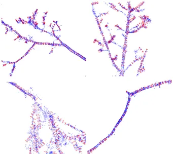
Figure 9: Cylinder fitting for branches. The upper branches are from deciduous tree and the bottom branches are from coniferous tree. The point clouds (blue points) are thinned out.
the fitting gives good approximation, see Fig. 8. For branches the fitting is usually less good because there are much less points that, furthermore, usually are not round the branch but cover only one side of the branch. In addition, the ‘noise level’ is larger compared to the size (see Fig. 9).
9 RESULTS AND DISCUSSION
The final step in our method is to approximate the total above-ground volume and branch size distribution from the cylinder fit-ting data (radius and height). In our examples, the calculated volume approximations are 0.26 and 0.23 cubic meters for the coniferous and the deciduous tree, respectively. These are proba-bly underestimations because parts of the trunk and branches are not covered in the point clouds. Furthermore, there are also lot of parts that are poorly covered by the point clouds and whose size we could not estimate. This was particularly true for the upper parts of the trees and for small branches (see the parts without fitted cylinders in Fig. 9).
The calculated branch size distributions, i.e., the length and
vol-0 2 4 6 8 10 12 14 16 18
1 1.5 2 2.5 3 3.5 4 4.5
Radius (cm)
log10 ( Length in centimeters )
leafy coniferous
0 2 4 6 8 10 12 14 16 18
0 0.01 0.02 0.03 0.04 0.05 0.06
Radius (cm)
Volume in cubic meters
leafy coniferous
Figure 10: Distributions of branch length (above) and volume (below) as functions of branch radius.
ume of the branches as functions of the branch radius, are shown in Fig. 10 (the trunks are also included in the distributions). The distributions show, as expected, that most segments, in terms of length, are in the branches of the smallest radii whereas most of the volume is in the trunk segments. There were no direct mea-surements of the branch sizes so the accuracy can be assessed only based on the visual inspection of the point cloud and fitted cylinders. The accuracy seems to be good for trunk parts and for thick branches that have many points. On the other hand, as ex-pected, for the smallest branches the accuracy is the poorest and approximations can have large relative errors. Particularly prob-lematic are the small branches of coniferous trees because of their needles. Deciduous trees probably have the same problem when there are leaves (our scan was from a deciduous tree without its leaves). However, the approximation errors of small branches may not be a problem if we are only interested in a size reso-lution of some centimeters. Furthermore, although the absolute distribution values may have quite large errors, the relative distri-bution values are probably more accurate, particularly if there are systematic errors that can be estimated fairly well.
10 CONCLUSIONS AND FUTURE WORK
sets is easy to modify for other applications where separation and recognition are important.
The method was demonstrated by computing approximations of the total above-ground volumes and branch size distributions of a deciduous tree and a coniferous tree. However, these demon-strations are only the beginning of future work in which the im-plementation of the method is developed further. Furthermore, the reliability and accuracy of the method and its realizations has to be analyzed. This includes, for example, the classification of the cover sets and how the classification depends on the size of the cover sets and the parameter values chosen for the geometric characterizations. The accuracy of the size approximations, par-ticularly for small branches with needles and leaves, must also be evaluated. Moreover, the dependency of the size approxima-tions and the classification on the number of points needs to be assessed. Also, the dependency of the total volume and branch size distribution approximations on the cover extent (the number of different scan positions) should be studied. The method and its implementations, in their many aspects, should also be compared with various other existing approaches.
ACKNOWLEDGEMENTS
This study was financially supported by the Academy of Finland projects: Modelling and applications of stochastic and regular surfaces in inverse problems and New techniques in active remote sensing: hyperspectral laser in environmental change detection.
REFERENCES
Gorte, B. G. H., Pfeifer, N. (2004). Structuring laser scanned trees using 3D mathematical morphology. International Archives of Photogrammetry, Remote Sensing and Spatial Information Sci-ences, 35: 929-933.
Lukacs, G., Martin, R., Marshall, D. (1998). Faithful least-squares fitting of spheres, cylinders and tori for reliable segmen-tation. Proceedings of the 5th European Conference on Computer Vision, 671-686.
Maas, H. -G., Bienert, A., Scheller, S., Keane, E. (2008). Au-tomatic forest inventory parameter determination from terres-trial laser scanner data. International Journal of Remote Sensing, 29(5): 1579-1593.
Madsen, K., Nielsen, H. B., Tingleff, O. (2004). Methods for Non-Linear Least Squares Problems (2nd ed.). Informatics and Mathematical Modelling, Technical University of Denmark, 60 pages.
Mitra, N. J., Nguyen, A., Guibas, L. (2004). Estimating Sur-face Normals in Noisy Point Cloud Data. International Journal of Computational Geometry and Applications, 14(4-5): 261-276.
Pfeifer, N., Gorte, B., Winterhalder, D. (2004). Automatic Re-construction of Single Trees from Terrestrial Laser Scanner Data. International Archives of Photogrammetry, Remote Sensing and Spatial Information Sciences, Istanbul, Turkey, 35(B5): 114-119.
Pfeifer, N., Winterhalder, D. (2004). Modelling of tree cross sec-tions from terrestrial laser-scanning data with free-form curves. International Archives of Photogrammetry, Remote Sensing and Spatial Information Sciences, 36: 76-81.