The next generation of low-cost personal air quality sensors for quantitative exposure monitoring

(1)

AMTD

7, 2425–2457, 2014

Next generation of low-cost personal air

quality sensors

R. Piedrahita et al.

Title Page

Abstract Introduction

Conclusions References

Tables Figures

◭ ◮

Back Close

Full Screen / Esc

Printer-friendly Version Interactive Discussion

Discussion

P

a

per

|

D

iscussion

P

a

per

|

Discussion

P

a

per

|

Discuss

ion

P

a

per

|

Atmos. Meas. Tech. Discuss., 7, 2425–2457, 2014 www.atmos-meas-tech-discuss.net/7/2425/2014/ doi:10.5194/amtd-7-2425-2014

Atmospheric Measurement

Techniques

Open Access

Discussions

This discussion paper is/has been under review for the journal Atmospheric Measurement Techniques (AMT). Please refer to the corresponding final paper in AMT if available.

The next generation of low-cost personal

air quality sensors for quantitative

exposure monitoring

R. Piedrahita1, Y. Xiang4, N. Masson1, J. Ortega1, A. Collier1, Y. Jiang2, K. Li3,

R. Dick4, Q. Lv2, M. Hannigan1, and L. Shang3

1

University of Colorado, Boulder, Department of Mechanical Engineering, 427 UCB, 1111 Engineering Drive, Boulder, CO, 80304, USA

2

University of Colorado, Boulder, Department of Computer Science, 430 UCB, 1111 Engineering Drive, Boulder, CO, 80304, USA

3

University of Colorado, Boulder, Department of Electrical Engineering, 425 UCB, 1111 Engineering Drive, Boulder, CO, 80304, USA

4

University of Michigan, Department of Electrical Engineering and Computer Science, 2417-E EECS, 1301 Beal Avenue, Ann Arbor, MI, USA

Received: 13 November 2013 – Accepted: 10 February 2014 – Published: 12 March 2014

Correspondence to: R. Piedrahita (ricardo.piedrahita@colorado.edu)

(2)

AMTD

7, 2425–2457, 2014

quality sensors

Title Page

Tables Figures

◭ ◮

Back Close

Full Screen / Esc

Discussion

P

a

per

|

D

iscussion

P

a

per

|

Discussion

P

a

per

|

Discuss

ion

P

a

per

|

Abstract

Advances in embedded systems and low-cost gas sensors are enabling a new wave of low cost air quality monitoring tools. Our team has been engaged in the development of low-cost wearable air quality monitors (Pods) using the Arduino platform. The M-Pods use commercially available metal oxide semiconductor (MO_x) sensors to measure

5

CO, O₃, NO₂, and total VOCs, and NDIR sensors to measure CO₂. MO_x sensors are low in cost and show high sensitivity near ambient levels; however they display non-linear output signals and have cross sensitivity e_ffects. Thus, a quantification system was developed to convert the MO_xsensor signals into concentrations.

Two deployments were conducted at a regulatory monitoring station in Denver,

Col-10

orado. M-Pod concentrations were determined using laboratory calibration techniques and co-location calibrations, in which we place the M-Pods near regulatory monitors to then derive calibration function coefficients using the regulatory monitors as the stan-dard. The form of the calibration function was derived based on laboratory experiments. We discuss various techniques used to estimate measurement uncertainties. A

sepa-15

rate user study was also conducted to assess personal exposure and M-Pod reliability. In this study, 10 M-Pods were calibrated via co-location multiple times over 4 weeks and sensor drift was analyzed with the result being a calibration function that included drift.

We found that co-location calibrations perform better than laboratory calibrations.

20

Lab calibrations su_ffer from bias and di_fficulty in covering the necessary parameter space. During co-location calibrations, median standard errors ranged between 4.0– 6.1 ppb for O₃, 6.4–8.4 ppb for NO₂, 0.28–0.44 ppm for CO, and 16.8 ppm for CO₂. Median signal to noise (S/N) ratios for the M-Pod sensors were higher for M-Pods than the regulatory instruments: for NO₂, 3.6 compared to 23.4; for O₃, 1.4 compared to 1.6;

25

(3)

AMTD

7, 2425–2457, 2014

quality sensors

Title Page

Tables Figures

◭ ◮

Back Close

Full Screen / Esc

Discussion

P

a

per

|

D

iscussion

P

a

per

|

Discussion

P

a

per

|

Discuss

ion

P

a

per

|

The user study provided trends and location-specific information on pollutants, and a_ffected change in user behavior. The study demonstrated the utility of the M-Pod as a tool to assess personal exposure.

1 Introduction

1.1 Background and motivation

5

Health effects such as asthma, cardio-pulmonary morbidity, cancer, and all-cause mor-tality are directly related to personal exposure of air pollutants (EPA ISA Health Criteria, 2010, 2013a, b). To comply with the US Clean Air Act, state monitoring agencies make ongoing measurements in centralized locations that are intended to be representative of the conditions normally experienced by the majority of the population. Because these

10

measurements require sophisticated, costly, and power-intensive equipment, they can only be taken at a limited number of sites. Depending on the pollutant, individual, and location, this limitation can lead to misleading personal exposure assessments (HEI, 2010). Low-cost, portable, and autonomous sensors have the potential to take equiv-alent measurements while more effectively capturing spatial variability and personal

15

exposure. Thus, we set out to survey such sensors, analyze their performance, and understand the feasibility of using them. We describe the M-Pod hardware and quan-tification system, and personal exposure results.

1.2 Low-cost portable air pollution measurement techniques

Quantitative measurements of pollutant concentrations generally require techniques to

20

(4)

AMTD

7, 2425–2457, 2014

quality sensors

Title Page

Tables Figures

◭ ◮

Back Close

Full Screen / Esc

Discussion

P

a

per

|

D

iscussion

P

a

per

|

Discussion

P

a

per

|

Discuss

ion

P

a

per

|

provide brief descriptions of the various techniques (along with their measurements, costs, and potential).

1.2.1 Carbon monoxide

Federal Reference Method (FRM) measurements of CO are made using infrared ab-sorption instruments, which use∼200 W power, cost $15 000–20 000, and require fre-5

quent calibrations and quality control checks (EPA Quality Assurance Handbook Vol. II, 2013). By comparison, metal oxide semiconductor (MO_x) sensors cost $5–15 and require less than 1 W of power. One example of this kind of device is the SGX 5525 sen-sor used for CO measurements that uses approximately∼80 mW power. MOxsensors

have fast responses, low detection limits, and require simple measurement circuitry.

10

However, they can have high cross-sensitivities to other reducing gases, and can be poisoned by certain gases or high doses of target gases. Daily or weekly calibrations are recommended.

The typical reducing gas MO_xsensor uses a heated tin-oxide n-type semi-conductor surface, on which oxygen can react with reducing gases, thus freeing electrons in the

15

semiconductor. This lowers the electrical resistance proportional to the concentration of the reducing gas (Moseley, 1997). These sensors suffer from cross-sensitivities to temperature, humidity, and other pollutants. Korotcenkov (2007) provides a compre-hensive review of MO_x materials and their characteristics for gas sensing, while Fine et al. (2010) and Bourgeois et al. (2003) review the use of MO_xsensors and arrays in

20

environmental monitoring.

Electrochemical sensors are relatively low in cost,∼$50–100, and have been used in

multiple studies that required low power sensors for measuring CO (Milton and Steed, 2007; Mead et al., 2013). They exhibit high sensitivity, low detection limit (sub-ppm for some models), fast response, low cross-sensitivity, and consume power in the

hun-25

(5)

AMTD

7, 2425–2457, 2014

quality sensors

Title Page

Tables Figures

◭ ◮

Back Close

Full Screen / Esc

Discussion

P

a

per

|

D

iscussion

P

a

per

|

Discussion

P

a

per

|

Discuss

ion

P

a

per

|

1.2.2 Ozone

FRM measurements of O₃ are made using the principle of chemiluminescence (EPA ISA, 2013a). Chemiluminescence instruments typically cost $10 000–20 000 and use approximately 1 kW. A Federal Equivalence Method uses UV absorption to measure an O₃concentration. Such instruments have prices in the low $1000 s.

5

MO_xO₃sensors have been commercialized and can cost anywhere from $5 to $100, with power consumption as low as 90 mW. A tungsten oxide semiconductor sensor board has been commercialized by Aeroqual, and costs∼$250. Power consumption is

2–6 W, and this material is reported to have less cross-sensitivity and drift than other MO_x materials (Williams et al., 2009). Electrochemical sensors are also available with

10

reported detection limits less than 5 ppb.

1.2.3 Nitrogen oxides (NOx)

FRM measurements of NO_x are made using the chemiluminescence reaction of O₃ with NO along with the catalytic reduction of NO₂ to NO (EPA ISA, 2013b). These instruments typically cost $10 000–20 000 and consume approximately 1 kW power.

15

NO₂can also be measured with electrochemical sensors ($80–210) and MO_xsensors ($4–54).

1.2.4 Carbon dioxide (CO2)

CO₂ is the primary anthropogenic greenhouse gas, as well as a proxy for assessing ventilation conditions in indoor environments. Elevated concentrations have also been

20

found to affect decision-making and exam performance (Satish et al., 2012). Portable non-dispersive infrared (NDIR) carbon dioxide sensors are precise, easy to calibrate, easy to integrate into a mobile sensing system (Yasuda et al., 2012), and are avail-able in the $40 range. The sensors operate by emitting a pulse of infrared radiation across a chamber. A detector at the other end of the chamber measures light intensity.

(6)

AMTD

7, 2425–2457, 2014

quality sensors

Title Page

Tables Figures

◭ ◮

Back Close

Full Screen / Esc

Discussion

P

a

per

|

D

iscussion

P

a

per

|

Discussion

P

a

per

|

Discuss

ion

P

a

per

|

Absorption of light by CO₂ accounts for the difference between expected and mea-sured intensity. Interference can occur due to absorption by water vapor and other gasses and drift can occur due to changes in the light source (Zakaria, 2010). Electro-chemical sensors are also available to measure CO₂. They are inexpensive and have low power requirements, but generally have slower response times, shorter lifespans,

5

and are more susceptible to poisoning and drift, than NDIR type sensors.

1.3 Instruments for personal air quality monitoring

Personal exposure has been characterized extensively using filter samplers, particle counters, and sorbent tubes. These methods can provide simple, accurate, and com-prehensive speciation results, but the time series information is lost since each filter or

10

adsorbent tube typically samples for durations of a day or more. Relatively recent sam-pling techniques allow for higher time-resolution personal measurement of pollutants.

Electrochemical sensors have been used to monitor CO in many works, including Kaur et al. (2007), Mead et al. (2013), Honicky et al. (2008), and Milton et al. (2006). Shum et al. (2011) developed a wearable CO, CO₂, and O₂monitor. O₃and NO_x have

15

both been monitored by Mead et al. and Honicky et al., using electrochemical and MO_x sensors. Williams et al. (2009) developed and deployed a portable tungsten oxide-based ozone sensor and NO₂sensor. Hasenfratz (2012) also monitored O₃in a train-mounted instrument study using metal oxide semiconductor sensors. Hasenfratz’s work tested collaborative calibration performance, in which sensor nodes were periodically

20

co-located to check and improve calibrations.

Tsow et al. (2011) developed wearable monitors to measure benzene, toluene, ethyl-benzene and xylene at ppb levels. The measurement is based on a MEMS tuning fork design that provides good selectivity and low detection limits, but the device is not yet commercially available. Electronic nose systems for sensing VOCs are commercially

25

(7)

AMTD

7, 2425–2457, 2014

quality sensors

Title Page

Tables Figures

◭ ◮

Back Close

Full Screen / Esc

Discussion

P

a

per

|

D

iscussion

P

a

per

|

Discussion

P

a

per

|

Discuss

ion

P

a

per

|

chromatography, among others (Röck et al., 2008). These models and most real-time personal exposure monitors are currently too expensive to be truly ubiquitous.

Advancements in technology and increasing concern about air quality in many gions have produced a wave of low-cost personal exposure instruments. Reliable re-sults are needed for users of these low cost monitors before they take action to reduce

5

their exposure. We describe our novel quantification system that includes co-location calibration, modeling of sensor responses with environmental parameters, and uncer-tainty estimation for these measurements. We demonstrate the quantification system by presenting results from a user study where six users wore monitors for 10–20 days.

2 Methods

10

2.1 MAQS – Mobile Air Quality Sensing System

The requirements for our mobile sensing system included wearability, low-cost, multi-pollutant (sensing of as many NAAQS criteria multi-pollutants at typical ambient concen-trations as possible), wireless communication, and enough battery life to wear for an entire day. The result of our development effort is the M-Pod, shown in Fig. 1.

15

The Mobile Air Quality Sensing (MAQS) system is designed to collect, analyze, and share air quality data (Jiang et al., 2011). An Android mobile phone application, MAQS3 (Mobile Air Quality Sensing v.3, 2014) pairs with the Pod via Bluetooth, and the M-Pod data is transmitted to the phone periodically. This data is then sent to a server for analysis. A web-based analysis and GIS visualization platform can access new

20

data from the server. Wi-Fi fingerprints can also be used to identify an M-Pod’s indoor locations (Jiang et al., 2012).

The M-Pod has four metal oxide sensors, measuring CO, total VOCs, NO₂, and O₃ (SGX Corporation models MiCS-5525, MiCS-5121WP, MiCS-2710, and MiCS-2611). Socket-mount MO_x sensors were used because of the di_fficulty replacing the

surface-25

(8)

AMTD

7, 2425–2457, 2014

quality sensors

Title Page

Tables Figures

◭ ◮

Back Close

Full Screen / Esc

Discussion

P

a

per

|

D

iscussion

P

a

per

|

Discussion

P

a

per

|

Discuss

ion

P

a

per

|

(hot-air reflow). An NDIR sensor (ELT, S100) measures CO₂and a fan (Copal F16EA-03LLC) provides steady flow through the device. Data is logged using an Arduino-based platform. The M-Pod also has a light sensor, and a relative humidity and tem-perature sensor (Sensirion, SHT21).

2.2 Calibration system

5

MO_x sensors represent the lowest cost sensing solution but hold significant quantifi-cation challenges. MO_x sensor responses are non-linear with respect to gas concen-tration, and are affected by ambient temperature and, to a lesser degree, by humidity (Sohn et al., 2008; Barsan and Weimar, 2001; Delpha et al., 1999). Baseline drift and changes to sensitivity over time are also common. These are typically due to aging

10

and irreversible changes to the sensing surface (Romain and Nicolas, 2009). As such, using MO_x sensors quantitatively requires that a model be developed which not only characterizes the relationship between sensor resistance and gas concentration, but also includes the impacts of these other parameters. Below we describe our calibration system and strategies for overcoming these challenges.

15

Our calibration system uses automated mass flow controllers (MFCs, Coastal Instru-ments FC-2902V) and solenoidal valves to inject specific mixtures of gas standards into a Teflon-coated aluminum chamber equipped with, temperature and relative hu-midity control. Custom LabVIEW software and Labjack data acquisition devices are used for instrument control and data logging. The CO and NO₂ sensors were

cali-20

brated for changes in temperature and humidity. The CO₂sensors were only calibrated for temperature, as they show a small non-linear response to temperature. Humidity ef-fects have been reported for NDIR sensors, but are not a significant issue in this case. Temperature is controlled using a heat lamp and by performing calibrations inside a re-frigerated chamber. Routing a portion of the airflow through deionized water controls

25

(9)

AMTD

7, 2425–2457, 2014

quality sensors

Title Page

Tables Figures

◭ ◮

Back Close

Full Screen / Esc

Discussion

P

a

per

|

D

iscussion

P

a

per

|

Discussion

P

a

per

|

Discuss

ion

P

a

per

|

run consists of different gas concentrations, temperature and humidity set points. Sen-sors are held at each state for periods of 15 min to allow them to reach steady state. The last 30 s of each 15 min period are averaged, and these points are used for the calibration. Initially, the sensors were calibrated by mounting them on large arrays, but we found that the sensor response is highly dependent on the position in the array and

5

air flow conditions. The convective cooling of the sensors is thus an important variable. To ensure that calibration temperature and flow conditions about each sensor are the same as during operating conditions, they are calibrated in their individual M-Pods.

2.3 Development of quantification models

To simplify the inter-comparison of MO_xsensors (which are often highly heterogeneous

10

from sensor to sensor), it is common practice to normalize a sensor’s resistance by a reference resistance,Ro. The reference resistance is the sensor’s unique response

to a given environment, for example, clean air at 25◦_{C, standard atmospheric pressure,} and 20 % relative humidity. As such, a sensor quantification model relates R_s/R_o to concentration, temperature and humidity. Previous works have used machine-learning

15

techniques to determine concentration values (Kamionka et al., 2006) and identify pol-lution sources (Gardner and Bartlett, 1994). However, to our knowledge, a parametric regression based model has yet to be developed for these sensors. We believe this type of model is preferable for ease of implementation.

Two sensor models were chosen for the majority of the analysis conducted thus far:

20

the MiCS-5121WP CO/VOC sensor and MiCS-5525 CO sensor (both manufactured by SGX Sensortech). The VOC sensor was chosen because of our strong initial interest in indoor air pollution. The MiCS-5525 was the logical next step because it has the same semiconductor sensor surface as the MiCS-5121, but with an activated charcoal pre-filter. The models to convert sensor signal to concentration were developed using both

25

(10)

AMTD

7, 2425–2457, 2014

quality sensors

Title Page

Tables Figures

◭ ◮

Back Close

Full Screen / Esc

Discussion

P

a

per

|

D

iscussion

P

a

per

|

Discussion

P

a

per

|

Discuss

ion

P

a

per

|

CO sensor used in the co-location. Our results show that the CO, NO₂ and O₃ MO_x sensors can detect ambient concentrations when frequently calibrated.

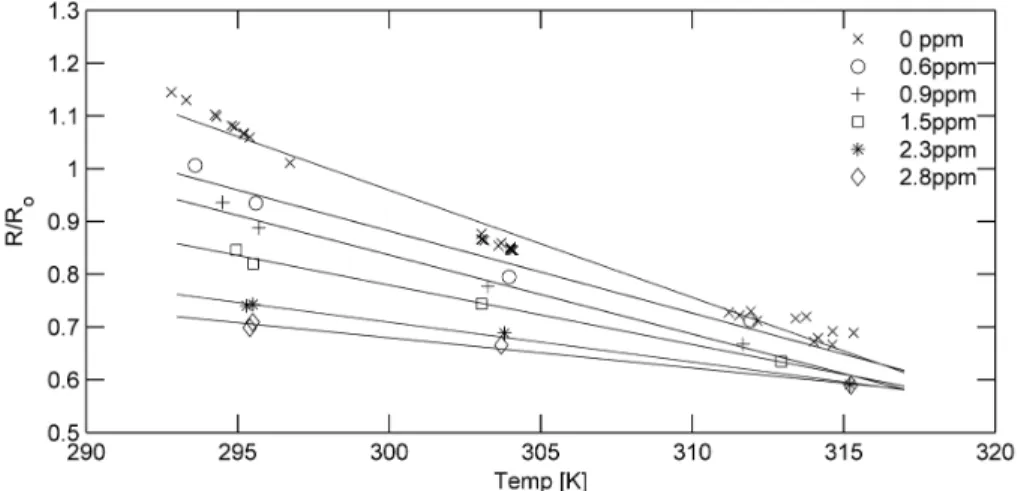
Figure 2 illustrates the MiCS-5525 CO sensor response to changing temperature at various concentrations of CO. The absolute humidity has a lesser effect on sig-nal response and was held constant so as to minimize the degrees of freedom within

5

the model response. From experimental observation, the sensor response appears to change linearly with respect to temperature for a given CO concentration between con-centrations of 0–2.8 ppm. The slope and intercept of the linear temperature trends also appear to decrease with increasing CO concentration. Equation (1) was chosen as the best fit for the observed sensor response to CO concentration and temperature. A third

10

term of the same form was added to the model to account for changes in absolute humidity (H).

R_s Ro=

f(C)(T−298)+g(C)+h(C)H (1)

In this model, f(C) describes the change in temperature slope with respect to

pollu-15

tant concentration; g(C) describes the change in resistance in dry air at 298 K due to concentration; and h(C) describes the change in absolute humidity slope with re-spect to concentration. The termsf(C),g(C), andh(C) were chosen to be of the form

p₁exp(Cp₂).

This model form performed well for all MO_x sensors used, but is computationally

20

challenging to work with because it is not algebraically invertible. Instead, we used a 2nd order Taylor approximation for this model. However, an even simpler model in temperature, absolute humidity, and concentration (Eq. 2) was found to perform sim-ilarly in many cases. The comparable performance of the models is likely due to the low variation in CO concentration observed throughout the field experiments. Though

25

(11)

AMTD

7, 2425–2457, 2014

quality sensors

Title Page

Tables Figures

◭ ◮

Back Close

Full Screen / Esc

Discussion

P

a

per

|

D

iscussion

P

a

per

|

Discussion

P

a

per

|

Discuss

ion

P

a

per

|

the model in Eq. (1).

R_s

R_o=p1+p2C+p3T+p4H (2)

In cases with longer time series and multiple calibrations, a time term,p₅t, was added to correct for temporal drift.

5

R_s Ro=

p₁+p₂C+p₃T+p₄H+p₅t (3)

Equation (3) was used throughout the results unless otherwise noted.

We determined concentration uncertainty by propagating the error in the calibration model through the inverted calibration function (NIST Engineering Statistics Handbook

10

2.3.6.7.1). The calculation included co-variance terms, but did not include the propa-gated uncertainty of the temperature, humidity, nor voltage measurements, as those are expected to be insignificant relative to the other sources of error. The calculated uncertainty does not directly account for sources of error such as convection heat loss or cross sensitivities that may be seen in field measurements but not during calibration.

15

However, co-location calibration should account for some cross-sensitivity e_ffects since there is simultaneous exposure to various measured pollutants.

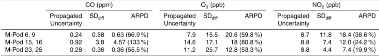
To explore the validity of this uncertainty propagation, we employed duplicate M-Pods during a user study. For this user study data, when there were duplicate M-Pod measurements but no reference monitors, we used two additional methods to explore

20

uncertainty, the average relative percent di_fference (ARPD), and the pooled pairwise standard deviation of the differences (SD_di_ff) (Table 4). These formulas are defined as follows:

SD_di_ff₌

v u u t

1 2n

n

X

i=1

C_iprimary−C_iduplicate

2

(4)

(12)

AMTD

7, 2425–2457, 2014

quality sensors

Title Page

Tables Figures

◭ ◮

Back Close

Full Screen / Esc

Discussion

P

a

per

|

D

iscussion

P

a

per

|

Discussion

P

a

per

|

Discuss

ion

P

a

per

|

ARPD₌2

n

X

i=1

C

primary

i −C

duplicate

i

C_iprimary+Cduplicate_i

×100 % (5)

This approach, outlined in Dutton et al. (2009), provides an additional assessment of measurement uncertainty, and can be compared to the uncertainties calculated using

5

propagation of error to understand if the propagation has captured most real sources of error. To calculate the ARPD, negative data were removed. In the future, zero replace-ment, or detection limit replacement for data with negative values will be considered. The ARPD was then multiplied by the average pooled concentration measurements to get units of concentration that could be directly compared with the uncertainty

esti-10

mates derived through propagation.

2.4 Validation and user study

From 3–12 December 2012, and later from 17–22 January 2013, nine M-Pods were co-located with reference instruments at a Colorado Department of Public Health and Environment (CDPHE) air monitoring station in downtown Denver. Total system

perfor-15

mance was assessed by comparing laboratory-generated calibrations with calibrations based on “real-world” ambient data, referred to as co-location calibrations. The 2nd co-location was performed with a fresh set of sensors and yielded slightly better re-sults (Supplement). Reference instruments for calibration and validation were provided by CDPHE and the National Center for Atmospheric Research (NCAR). CO was

mea-20

sured using a Thermo Electron 48c monitor, CO₂and H₂O were measured with a LI-COR LI-6262, NO₂was measured using a Teledyne 200E, and O₃was measured with a Teledyne 400E. The CO₂instrument was calibrated before the deployment, while the others were span and zero checked daily as per CDPHE protocol. The M-Pods were positioned 8 feet from the sampling inlets. They operated continuously in a ventilated

25

(13)

AMTD

7, 2425–2457, 2014

quality sensors

Title Page

Tables Figures

◭ ◮

Back Close

Full Screen / Esc

Discussion

P

a

per

|

D

iscussion

P

a

per

|

Discussion

P

a

per

|

Discuss

ion

P

a

per

|

In the user-study portion of the validation, nine M-Pods were carried for over two weeks, with three users each carrying two M-Pods. The objective of the user study was to demonstrate the use of the M-Pods for assessing personal exposure. Specifically, we were interested in M-Pod inter-comparisons and how they drift over time during personal usage. The M-Pods were calibrated before and after the deployment using

co-5

location calibrations. They were worn on the user’s upper arm or attached to backpacks or bags, and were placed as close as possible to the breathing area when users were sitting or sleeping.

Measurement values were given as minute medians of the 1/10 Hz raw data. The raw data was filtered beforehand for electronic noise. Sensor-specific thresholds of two

10

standard deviations on the di_fferences between sequential values were used to identify and remove noise spikes. An upper bound threshold on sequential di_fferences provided another layer of filtering for the noisiest data. To ensure that sensors were warmed up, 10 min of data were removed after power-on. Additional noise filtering was applied for the co-location tests due to a bad USB power supply. This data was filtered for noise

15

by applying the Grubbs test for outliers to the di_fferences between all the M-Pods and a “reference” M-Pod that displayed less electronic noise.

3 Results

3.1 Lab vs. co-location calibration results

A summary of the results from the 3–12 December co-location and lab-calibrated data

20

(14)

AMTD

7, 2425–2457, 2014

quality sensors

Title Page

Tables Figures

◭ ◮

Back Close

Full Screen / Esc

Discussion

P

a

per

|

D

iscussion

P

a

per

|

Discussion

P

a

per

|

Discuss

ion

P

a

per

|

3.1.1 MOxsensor results

The MiCS-5525 CO sensor was found to have substantially higher error using lab-calibrations vs. co-location lab-calibrations. As shown in Table 1, the median standard error for co-location calibration was 0.45 ppm (range 0.38–0.52 ppm), while the median lab calibration standard error was 3.56 ppm (range 2.85–5.33 ppm). Adding a linear time

5

correction, as in Eq. (3), was found to improve the fit in most MO_x sensor data sets. In this case, it improved the fit of the co-location calibrations slightly, giving a median standard error of 0.44 ppm (range 0.38–0.51 ppm). The median standard error for the exponential-based model from Eq. (1) was 0.39 ppm (range 0.34–1.78 ppm), but it ac-tually provided a worse fit in some cases. The linear form of the equation, Eq. (2),

10

is a good approximation of the exponential form shown in Eq. (1), likely because of the small parameter space spanned by the observed data. We have included residual plots (Fig. 3) to demonstrate model performance. Note the absence of a trend in these residual plots.

The relationship between co-location calibrated sensor readings and reference data

15

showed a slight negative bias at the higher end of observed concentration levels, but this appears to be driven by a small number of data points.

Inter-sensor variability is of interest if these sensors are to be widely deployed. Low variability could allow us to calibrate fewer sensors and apply those calibrations to other sensors in a large network. Inter-sensor variability for CO was generally low, with

20

median correlation coe_fficients among the M-Pods 0.70 (range 0.62–0.78). The median signal to noise (S/N) ratio, defined as the median observed value over the standard error, was 1.13 (range 1.00–1.26). This compares with the reference instrumentS/N of 10.0, calculated using the median standard error from multiple days of zero and span-check data as noise. TheS/Nratio provides straightforward comparison of instruments,

25

and shows us how often the measurements are above the noise.

(15)

AMTD

7, 2425–2457, 2014

quality sensors

Title Page

Tables Figures

◭ ◮

Back Close

Full Screen / Esc

Discussion

P

a

per

|

D

iscussion

P

a

per

|

Discussion

P

a

per

|

Discuss

ion

P

a

per

|

(range 6.9–9.5 ppb), respectively. As shown in Table 2, the linear model from Eq. (2) was found to fit the data nearly as well for NO₂ as the non-linear model from Eq. (1), and is much less computationally intensive to use. An NO₂example time series using the linear model from Eq. (2) is shown in Fig. 3. The non-linear model was not able to fit the O₃ data with any success, also shown in Table 2. The reason for this was

5

not determined despite repeated testing. Lab calibrations were not performed for O₃ and NO₂. Median inter-sensor correlation for O₃was 0.83 (range 0.46–0.99), and 0.96 (range 0.94–0.99) for NO₂. The median NO₂S/N was 3.6 (range 3.3–4.4), compared with the median reference instrument S/N of 23.4. For O₃, the medianS/N ratio for the M-Pods was 1.4 (range 0.5–2.0), while the reference instrument hadS/N of 1.6.

10

Figure 3 NO₂data from M-Pod 23 from the December co-location.

3.1.2 NDIR CO2sensor results

CO₂values quantified with lab calibrations showed bias in some M-Pods (see Table 2), while others showed a high degree of accuracy. With co-location calibration, we also found a previously unseen temperature e_ffect, described by

15

v=p1+p2C+p3(T−p4)2, (6)

wherev is the raw sensor signal. This model fit better than a linear model in concen-tration, and an example is shown in Fig. 4.

As shown in Table 2, using linear models in concentration only, the median standard

20

error for M-Pod CO₂ measurements using the lab calibrations was 68.4 ppm (range 15.2–138.7 ppm), and was 16.8 ppm (range 10.1–48.8 ppm) using the co-location cal-ibration. Median standard error was 10.9 ppm (range 7.2–24.8 ppm) using the co-location calibration model from Eq. (6), and adding a linear time correction to this model further improved the fit, dropping the median standard error to 6.9 ppm. This drift term

25

(16)

AMTD

7, 2425–2457, 2014

quality sensors

Title Page

Tables Figures

◭ ◮

Back Close

Full Screen / Esc

Discussion

P

a

per

|

D

iscussion

P

a

per

|

Discussion

P

a

per

|

Discuss

ion

P

a

per

|

fit significantly. Using the co-location calibration approach, the median correlation be-tween CO₂sensors in di_fferent M-Pods was 0.88 (range 0.58–0.98). The median signal to noise ratio was 42.2 (range 18.5–63.4), as compared with a reported 300–500 from the reference instrument used (LICOR, 1996).

3.2 User-study results

5

Based on initial lab and co-location calibration results, calibrations for the user-study were performed only with co-location calibrations. Co-location calibrations were carried out before and after the 3-week measurement period. Calibration fits were comparable to the prior co-location calibrations for CO (median standard error of 0.3 ppm), NO₂ (median standard error of 8.8 ppb), and O₃ (median standard error of 9.7 ppb). For

10

CO₂, the median standard error was high (36.9 ppm), likely because we were unable to co-locate a reference monitor with the M-Pods at these times. Instead, a calibration curve was generated using data from a nearby ambient monitor operated by NCAR and a lab calibration. Correlations among paired M-Pods during the user study ranged between 0.88–0.90 for NO₂, 0.48–0.76 for CO, 0.33–0.92 for CO₂, and 0.04–0.35 for

15

O₃. The range of correlations for CO₂was due to power supply issues, which will be discussed later. We expect reliable CO₂sensor performance to be easily achievable in future work. Despite the low standard error from O₃sensor calibrations, we found low correlations among the paired M-Pods during the user study, which is also likely due to a power supply issue.

20

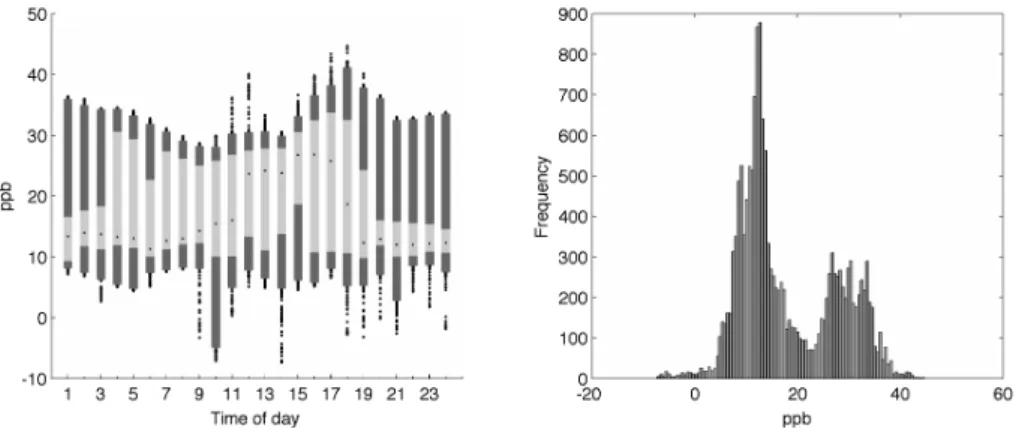
Personal exposure measurements using the M-Pods were generally low for all users, but clear trends and e_ffects of behavior were seen. Table 3 shows summary statistics. Median CO and CO₂exposure were 0.58 ppm and 949.0 ppm, respectively. Median O₃ exposure was 14.0 ppb, and Fig. 5 has an example probability density plot and time of day trend plot for a user’s O₃exposure.

25

(17)

AMTD

7, 2425–2457, 2014

quality sensors

Title Page

Tables Figures

◭ ◮

Back Close

Full Screen / Esc

Discussion

P

a

per

|

D

iscussion

P

a

per

|

Discussion

P

a

per

|

Discuss

ion

P

a

per

|

For CO and O₃, the propagated uncertainty is lower than the SD_di_ffand ARPD, roughly 50–75 % of it, confirming that there are sources of error that are not accounted for in the uncertainty propagation. For NO₂, the propagated measurement uncertainty seems to capture most of the uncertainty observed in the pairs. The RMSE values from the sensor calibrations were found to account for the majority of the propagated error.

Fig-5

ure 6 compares the CO measurements from M-Pods 23 and 25, along with their 95 % confidence interval, the ARPD, and SD_di_ff.

Drift was seen to a_ffect the measurement results, as described in detail in the Sup-plement. We compensated for drift using multiple co-location calibrations with linear time corrections (Haugen et al., 2000), and observed improved calibration fits. Average

10

daily drift during the user study is shown in Table 3. For CO, all M-Pods experienced drift under−0.05 ppm day−1, apart from M-Pod 15, which showed behavior we cannot

explain. O₃sensors experienced between−2.6 ppb day−1and 2.0 ppb day−1drift. CO2

drift ranged from−4.2 ppm day−1 to 3.1 ppm day−1, excluding the bad results from

M-Pod 9. NO₂generally showed a slight positive drift over time, with a range of−1.56 to 15

0.51 ppb day−1_.

4 Discussion

The M-Pods performed well given the relatively low ambient concentration environ-ments encountered in the region. For CO, NO₂, and CO₂, the reference instruments exhibited S/N ratios 8–10 times higher than the M-Pod measurements. For O₃, the

20

reference monitorS/Nratio was only slightly higher than the median M-Pod value. The user study demonstrated the utility of the M-Pod in real time continuous monitoring applications, in terms of user behavior changes. For example, one user experienced elevated nighttime CO₂and NO₂. CO₂levels often increase at night in rooms with little ventilation, and can lead to restlessness. NO₂levels increase due to combustion, and

25

(18)

AMTD

7, 2425–2457, 2014

quality sensors

Title Page

Tables Figures

◭ ◮

Back Close

Full Screen / Esc

Discussion

P

a

per

|

D

iscussion

P

a

per

|

Discussion

P

a

per

|

Discuss

ion

P

a

per

|

personal NO₂ exposure substantially. With this kind of readily available concentration data, users can then adjust their behavior to reduce night time exposures.

4.1 Lab calibration

Lab calibrations had higher measurement error than co-location calibrations, likely be-cause the field data covered a wider range of environmental parameter space than

5

the lab calibration. The poor performance of lab calibrations may also be due to the di_fference between zero-grade air cylinders and ambient air. Conducting co-location calibrations in the region of interest helps to account for confounding factors and me-teorological variability.

CO₂lab-calibration results showed accurate results in some cases, while in other

M-10

Pods we found significant bias. Some CO₂sensors consistently showed worse perfor-mance than others. Strangely, the worse performing ones were usually in good agree-ment with each other. We have no explanation for this behavior, apart from a potential power supply issue.

4.2 Co-location calibration

15

The time and resources required for lab calibration, and the di_fficulty reconciling the lab and ambient results, led us to rely more on co-location calibration. Co-location cal-ibration performed well during two wintertime tests. However, during later co-location calibrations in warmer periods with rapidly changing weather, we found more interfer-ence from either reducing gases or humidity swings than we had previously seen. This

20

effect, coupled with generally lower CO levels in the warmer months due to better atmo-spheric mixing and improved motor vehicle combustion (Ne_ffet al., 1997), resulted in flatter and noisier calibration curves than previously seen. To minimize this e_ffect, some portions of the calibration data set were removed for April and May user study calibra-tions. O₃and NO₂had slightly worse calibration fits than during the winter calibrations,

25

(19)

AMTD

7, 2425–2457, 2014

quality sensors

Title Page

Tables Figures

◭ ◮

Back Close

Full Screen / Esc

Discussion

P

a

per

|

D

iscussion

P

a

per

|

Discussion

P

a

per

|

Discuss

ion

P

a

per

|

4.3 User study discussion

The user study provided valuable insight and promoted changes in behavior of some participants. Users reported being more aware of “stu_ffiness”, and acted based on their data by opening windows to increase air exchange rates in their homes. They also noted increases in CO₂, CO, and NO₂during driving, leading them to experiment

5

with the best way to reduce exposures.S/N ratios during the user study were gener-ally higher than during the co-locations. This suggests that during personal exposure measurement, when concentration peaks are often higher than background measure-ments, the M-Pod is able to detect those peaks above the noise. Analysis based on the propagated uncertainty, ARPD, and SD_di_ff suggests that propagated uncertainty

10

is capturing most sources of error, but it does require more testing to further validate uncertainty estimation approaches.

Temporal trends generally showed higher concentrations in the morning and evening for CO and NO₂, coinciding with commute-time increases in ambient concentrations. O₃trends followed expected outdoor patterns, peaking in the afternoon in most cases.

15

CO₂ trends generally showed nighttime increases. The distributions had a distinct “fresh air” mode, near ambient concentrations, and an indoor mode with a heavy tail. For other pollutants, exposure probability density function distributions varied substan-tially, likely due to exposure variability based on individual user behavior. One user’s overnight use of a wood-fired stove is evident with increased nighttime CO exposure

20

and a wider distribution than that of other users. Most other CO distributions were quite narrow, though slightly right-skewed. The NO₂distributions varied between right-skewed distributions for four Pods, and bi-modal distributions for the other five M-Pods. These modes appear to be driven by daily di_fferences in NO₂ exposure rather than indoor/outdoor differences.

25

(20)

AMTD

7, 2425–2457, 2014

quality sensors

Title Page

Tables Figures

◭ ◮

Back Close

Full Screen / Esc

Discussion

P

a

per

|

D

iscussion

P

a

per

|

Discussion

P

a

per

|

Discuss

ion

P

a

per

|

the perceived value of the M-Pod. Unfortunately, one M-Pod from each of two of the M-Pod pairs appears to have had persistent power issues, which would explain the low number of samples relative to their respective pairs, and worse sensor behavior during calibration.

A study shortcoming was the inability to wear reference monitors in addition to the

M-5

Pods. This was illustrated with curiously high NO₂concentrations, indicating that there may be problems we are not accounting for. Despite such potential issues, concentra-tion changes near busy roadways are often apparent, showing the sensitivity and fast response of the sensors, valuable for source and trend identification.

5 Conclusions

10

Co-location and collaborative calibration will be a valuable tool in the next generation of air quality monitoring. With help from monitoring agencies and citizen scientists, detailed ground-level pollutant maps will one day help track sources, reduce the pop-ulation’s exposure, and improve our knowledge of emissions as well as fate for each species. In this work, we have demonstrated a quantification system that can provide

15

personal exposure measurements and uncertainties for CO₂, O₃, NO₂, and CO. This type of quantification approach provides access to air quality monitoring to a wider audi-ence of scientists and citizens. It requires moderate investment to develop a calibration infrastructure, whether in a laboratory or near a monitoring station, but we believe it is worthwhile in applications like health and exposure, source identification, and leak

20

detection.

Supplementary material related to this article is available online at http://www.atmos-meas-tech-discuss.net/7/2425/2014/

(21)

AMTD

7, 2425–2457, 2014

quality sensors

Title Page

Tables Figures

◭ ◮

Back Close

Full Screen / Esc

Discussion

P

a

per

|

D

iscussion

P

a

per

|

Discussion

P

a

per

|

Discuss

ion

P

a

per

|

Acknowledgements. This work was funded by CNS awards O910995 & 0910816 from the Na-tional Science Foundation. Thank you to Bradley Rink and the CDPHE. Thank you to the Han-nigan Lab: Tiffany Duhl, Lamar Blackwell, Evan Coffey, Joanna Gordon, Nicholas Clements, and Kyle Karber.

References

5

Barsan, N. and Weimar, U.: Conduction model of metal oxide gas sensors, J. Electroceram., 7, 143–167, 2001.

Bourgeois, W., Romain, A. C., Nicolas, J., and Stuetz, R. M.: The use of sensor arrays for environmental monitoring: interests and limitations, J. Environ. Monitor., 5, 852–860, 2003. Delpha, C., Siadat, M., and Lumbreras, M.: Humidity dependence of a TGS gas sensor array

10

in an air-conditioned atmosphere, Sensor. Actuat. B-Chemical, 59, 255–259, 1999.

Dutton, S. J., Schauer, J. J., Vedal, S., and Hannigan, M. P.: PM_2.5Characterization for time se-ries studies: pointwise uncertainty estimation and bulk speciation methods applied in Denver, Atmos. Environ., 43, 1136–1146, 2009.

Fine, G. F., Cavanagh, L. M., Afonja, A., and Binions, R.: Metal oxide semi-conductor gas

15

sensors in environmental monitoring, Sensors, 10, 5469–5502, 2010.

Hasenfratz, D., Saukh, O., Sturzenegger, S., and Thiele, L.: Participatory air pollution monitoring using smartphones, in: Proc., 1st Int’l Workshop on Mobile Sensing: From Smartphones and Wearables to Big Data, 2012.

Haugen, J. E., Tomic, O., and Kvaal, K.: A calibration method for handling the temporal drift of

20

solid state gas-sensors, Anal. Chim. Acta, 407, 23–39, 2000.

Honicky, R. J., Mainwaring, A., Myers, C., Paulos, E., Subramanian, S., Woodruff, A., and Aoki, P.: Common Sense: Mobile Environmental Sensing Platforms to Support Community Action and Citizen Science, Human-Computer Interaction Institute, 2008.

HEI: Traffic-Related Air Pollution: A Critical Review of the Literature on Emissions, Exposure,

25

and Health Effects, Health Effects Institute, Boston, 2010.

Jiang, Y., Li, K., Tian, L., Piedrahita, R., Yun, X., Mansata, O., Lv, Q., Dick, R. P., Hannigan, M., and Shang, L.: MAQS: a mobile sensing system for indoor air quality, in: Proceedings of the 13th International Conference on Ubiquitous Computing, UbiComp 2011, ACM, New York, NY, USA, 493–494, 2011.

(22)

AMTD

7, 2425–2457, 2014

quality sensors

Title Page

Tables Figures

◭ ◮

Back Close

Full Screen / Esc

Discussion

P

a

per

|

D

iscussion

P

a

per

|

Discussion

P

a

per

|

Discuss

ion

P

a

per

|

Jiang, Y., Pan, X., Li, K., Lv, Q., Dick, R., Hannigan, M., and Shang, L.: ARIEL: automatic wi-fi based room fingerprinting for indoor localization, in: Proceedings of the 2012 ACM Conference on Ubiquitous Computing, UbiComp ’12, ACM, New York, NY, USA, 441–450, doi:10.1145/2370216.2370282, 2012.

Kaur, S., Nieuwenhuijsen, M. J., and Colvile, R. N.: Fine particulate matter and carbon

monox-5

ide exposure concentrations in urban street transport microenvironments, Atmos. Environ., 41, 4781–4810, 2007.

Korotcenkov, G.: Metal oxides for solid-state gas sensors: what determines our choice?, Mater. Sci. Eng., 139, 1–23, 2007.

MAQS Website: http://car.colorado.edu:443, last access: 9 March 2014.

10

Mead, M. I., Popoola, O. A. M., Stewart, G. B., Landshoff, P., Calleja, M., Hayes, M., Bal-dovi, J. J., McLeod, M. W., Hodgson, T. F., Dicks, J., Lewis, A., Cohen, J., Baron, R., Saffell, J. R., and Jones, R. L.: The use of electrochemical sensors for monitor-ing urban air quality in low-cost, high-density networks, Atmos. Environ., 70, 186–203, doi:10.1016/j.atmosenv.2012.11.060, 2013.

15

Milton, R. and Steed, A.: Mapping carbon monoxide using GPS tracked sensors, Environ. Monit. Assess., 124, 1–19, 2006.

Moseley, P. T.: Review article: solid state gas sensors, Measurement Science and Technology, 8, 223–237, 1997.

Neff, W. D.: The Denver Brown Cloud Studies from the perspective of model assessment needs

20

and the role of meteorology, J. Air Waste Manage., 47, 269–285, 1997.

Röck, F., Barsan, N., and Weimar, U.: Electronic nose: current status and future trends, Chem. Rev., 108, 705–725, 2008.

Romain, A. C. and Nicolas, J.: Long term stability of metal oxide-based gas sensors for e-nose environmental applications: an overview, Sensor. Actuat. B-Chemical, 146, 502–506, 2010.

25

Satish, U., Mendell, M. J., Shekhar, K., Hotchi, T., Sullivan, D., Streufert, S., Fisk, W., and Bill J.: Is CO2 an indoor pollutant? Direct effects of low-to-moderate CO2

concentra-tions on human decision-making performance, Environ. Health Persp., 120, 1671–1677, doi:10.1289/ehp.1104789, 2012.

Shum, L. V., Rajalakshmi, P., Afonja, A., McPhillips, G., Binions, R., Cheng, L., and Hailes, S.:

30

(23)

AMTD

7, 2425–2457, 2014

quality sensors

Title Page

Tables Figures

◭ ◮

Back Close

Full Screen / Esc

Discussion

P

a

per

|

D

iscussion

P

a

per

|

Discussion

P

a

per

|

Discuss

ion

P

a

per

|

Sohn, J. H., Atzeni, M., Zeller, L., and Pioggia, G.: Characterisation of humidity dependence of a metal oxide semiconductor sensor array using partial least squares, Sensor. Actuat. B-Chemical, 131, 230–235, 2008.

US EPA National Center for Environmental Assessment, R. T. P. N. and Brown, J.: Inte-grated Science Assessment of Ozone and Related Photochemical Oxidants (Final

Re-5

port), available at: http://cfpub.epa.gov/ncea/isa/recordisplay.cfm?deid=247492 (last access: 9 March 2014), 2013a.

US EPA National Center for Environmental Assessment, R. T. P. N. and Long, T.: Integrated Science Assessment for Carbon Monoxide (Final Report), avaliable at: http://cfpub.epa.gov/ ncea/isa/recordisplay.cfm?deid=218686 (last access: 9 March 2014), 2010.

10

US EPA National Center for Environmental Assessment, R. T. P. N. and Luben, T.: Integrated Science Assessment for Oxides of Nitrogen – Health Criteria (Final Report), available at: http://cfpub.epa.gov/ncea/cfm/recordisplay.cfm?deid=194645 (last access: 9 March 2014), 2013b.

Williams, D. E., Henshaw, G., Wells, D. B., Ding, G., Wagner, J., Wright, B., Yung, Y. F., Akagi, J.,

15

and Salmond, J.: Development of low-cost ozone and nitrogen dioxide measurement instru-ments suitable for use in an air quality monitoring network, in: ECS Transactions, Presented at the 215th ECS Meeting, San Francisco, CA, 251–254, 2009.

Yasuda, T., Yonemura, S., and Tani, A.: Comparison of the characteristics of small commer-cial NDIR CO₂ sensor models and development of a portable CO₂ measurement device,

20

Sensors, 12, 3641–3655, 2012.

(24)

AMTD

7, 2425–2457, 2014

quality sensors

Title Page

Tables Figures

◭ ◮

Back Close

Full Screen / Esc

Discussion

P

a

per

|

D

iscussion

P

a

per

|

Discussion

P

a

per

|

Discuss

ion

P

a

per

|

Table 1.Co-location calibration summary statistics for December co-location using the linear model from Eq. (3).

CO (ppm) O3(ppb)

N mean std med 5th % 95 % drift S/N N mean std med 5th % 95 % drift S/N

(ppb day−1₎ _{(ppm day}−1₎

M-Pod 1 14 157 0.59 0.69 0.47 −0.18 1.87 0.02 1.22 12 919 11.8 18.4 9.7 −9.2 41.1 −0.6 0.7

M-Pod 13 13 835 0.60 0.71 0.47 −0.23 1.92 −0.01 1.14 13 987 13.1 12.8 9.9 −2.8 36.0 −0.4 1.8

M-Pod 15 13 769 0.60 0.76 0.47 −0.26 2.00 0.03 1.00 11 749 10.5 18.3 7.9 −9.1 37.5 −0.4 0.5

M-Pod 17 14 006 0.60 0.74 0.49 −0.29 1.91 −0.01 1.11 13 365 12.2 12.9 9.0 −3.9 35.2 −0.3 1.4 M-Pod 18 13 976 0.60 0.69 0.47 −0.16 1.90 −0.03 1.26 14 090 13.0 15.0 9.9 −4.6 38.2 −0.3 1.0

M-Pod 19 14 097 0.60 0.78 0.52 −0.39 1.98 −0.02 1.03 13 451 12.2 12.8 8.3 −3.2 35.6 −0.1 1.4

M-Pod 21 14 007 0.60 0.75 0.51 −0.32 1.90 −0.05 1.09 13 365 12.2 12.2 8.2 −2.0 32.5 −0.1 2.0

M-Pod 23 14 013 0.60 0.74 0.50 −0.30 1.95 −0.03 1.14 13 368 12.2 12.2 8.3 −2.1 33.2 −0.2 1.9

Median 14 007 0.60 0.74 0.48 −0.27 1.92 −0.01 1.13 13 366.5 12.2 12.9 8.7 −3.6 35.8 −0.3 1.4

NO2(ppb) CO2(ppm)

N mean std med 5th % 95 % drift S/N N mean std med 5th % 95 % drift S/N

(ppb day−1₎ _{(ppm day}−1₎

M-Pod 1 14 157 29.3 16.3 30.4 3.1 52.3 −0.3 3.7 14 318 466.8 45.0 453.7 426.6 558.5 −1.5 53.9

M-Pod 13 14 311 466.8 46.7 455.1 418.1 562.4 −2.8 27.2

M-Pod 15 14 188 466.4 44.8 454.0 423.7 555.6 −1.6 47.6

M-Pod 17 13 997 29.4 17.0 30.3 0.4 53.0 0.3 3.2 14 295 466.9 44.8 454.2 426.0 557.0 −0.7 63.4

M-Pod 18 14 079 29.4 16.8 29.6 1.8 53.9 −0.9 3.4 14 080 466.7 44.9 453.6 427.2 561.2 −1.2 57.7 M-Pod 19 14 096 29.4 16.6 30.6 1.8 53.0 0.0 3.5 14 309 466.8 45.5 453.3 424.4 557.9 −2.3 36.9

M-Pod 21 13 883 29.3 16.2 30.5 3.1 51.7 −0.4 3.8 14 311 466.8 48.1 456.8 411.9 558.5 0.3 24.7

M-Pod 23 14 013 29.2 15.8 30.3 4.4 51.9 −0.5 4.4 14 311 467.3 50.4 457.1 410.9 573.4 −1.5 18.5

(25)

AMTD

7, 2425–2457, 2014

quality sensors

Title Page

Tables Figures

◭ ◮

Back Close

Full Screen / Esc

Discussion

P

a

per

|

D

iscussion

P

a

per

|

Discussion

P

a

per

|

Discuss

ion

P

a

per

|

Table 2. Standard errors for the various calibration models tested with the December co-location data set. Equation (1), the exponential model, was not able to fit O₃satisfactorily for some unknown reason.

CO2(ppm) CO (ppm) O3(ppb) NO2(ppb)

Calibration Co- Co- Co- Lab Co- Co- Co- Lab Co- Co- Co- Co- Co-

Co-type Model location location location location location location location location location location location location

Eq. (6) Eq. (6) w/time Linear Linear Eq. (1) Eq. (2) Eq. (3) Eq. (1) Eq. (1) Eq. (2) Eq. (3) Eq. (1) Eq. (2) Eq. (3)

M-Pod 1 8.4 7.3 11.0 138.7 0.38 0.38 0.38 3.69 68 413.9 15.4 14.9 7.2 8.2 8.2

M-Pod 13 16.8 14.4 18.2 29.1 0.39 0.42 0.41 3.54 37 558.7 5.6 5.4

M-Pod 15 9.5 8.4 10.1 43.3 0.42 0.46 0.46 2.85 249.771 15.3 14.9

M-Pod 17 7.2 6.9 15.5 15.2 0.35 0.44 0.44 3.22 60 671.4 6.4 6.2 7.5 9.5 9.5

M-Pod 18 7.9 7.1 10.5 30.0 0.34 0.38 0.37 3.58 3952.56 9.8 9.6 7.9 9.0 8.8

M-Pod 19 12.3 10.4 31.4 125.3 1.78 0.52 0.51 4.49 82 843.3 5.8 5.8 7.0 8.6 8.6

M-Pod 21 18.5 18.6 22.4 105.0 0.73 0.49 0.47 3.42 215.551 4.2 4.1 6.9 8.0 7.9

M-Pod 23 24.8 23.9 48.8 93.5 0.39 0.45 0.44 5.33 8569.4 4.4 4.4 6.0 6.9 6.8

(26)

AMTD

7, 2425–2457, 2014

quality sensors

Title Page

Tables Figures

◭ ◮

Back Close

Full Screen / Esc

Discussion

P

a

per

|

D

iscussion

P

a

per

|

Discussion

P

a

per

|

Discuss

ion

P

a

per

|

Table 3.Personal exposure summary statistics using the model in Eq. (3). Rows in italic/bold indicate paired M-Pods.

CO (ppm) O3(ppb)

N mean std med 5 % 95 % R2 _Drift

S/N N mean std med 5 % 95 % R2 _Drift

S/N

ppm day−1 _{ppm day}−1

M-Pod 4 17 107 0.52 0.62 0.37 −0.14 1.76 1.63 1.63 17 107 32.7 12.5 33.4 14.4 53.6 1.4 0.9

M-Pod 6 10 595 0.47 1.30 0.48 −0.66 2.18 0.48 1.52 1.52 10 595 14.6 13.7 12.3 −2.1 44.2 0.35 0.0 3.1

M-Pod 9 7214 1.26 0.68 1.27 0.11 2.17 7.18 7.18 7214 32.8 15.6 31.3 11.7 55.2 −0.5 3.0

M-Pod 15 8710 8.83 1.27 8.90 6.47 10.59 0.50 6.09 6.09 8710 15.4 18.3 17.5 −11.2 43.2 0.04 2.0 0.7

M-Pod 16 10 308 1.54 0.60 1.54 0.51 2.48 4.58 4.58 10 308 31.8 5.5 31.6 23.7 43.4 −0.5 3.7

M-Pod 17 11 816 −0.15 0.53 −0.14 −0.97 0.74 −0.36 −0.36 11 816 10.2 6.0 9.7 3.0 21.0 0.2 2.0

M-Pod 20 6265 −48.4 28.2 −53.7 −79.6 11.3 −2.6 −1.3

M-Pod 23 16 322 0.77 0.57 0.68 0.04 1.78 0.76 2.71 2.71 16 322 17.9 9.4 14.0 6.5 34.2 0.24 0.2 3.6 M-Pod 25 15 097 0.34 0.78 0.21 −0.59 1.78 1.22 1.22 15 097 −14.1 35.2 −8.1 −77.6 43.8 −1.3 −0.3

Median 11 205.5 0.64 0.65 0.58 −0.05 1.98 0.50 1.63 1.63 10 595 15.4 13.7 14.0 3.0 43.4 0.24 0.0 2.0

NO2(ppb) CO2(ppm)

N mean std med 5 % 95 % R2 _Drift

S/N N mean std med 5 % 95 % R2 _Drift

S/N

ppm day−1 _{ppm day}−1

M-Pod 4 17 107 69.0 9.5 68.7 54.2 83.3 −0.1 6.3 17 783 1108.6 367.2 1123.7 492.0 1772.2 −0.3 41.3

M-Pod 6 10 595 48.7 29.2 45.5 −12.3 86.0 0.88 0.2 4.0 10 910 902.3 544.5 807.8 374.9 1893.3 0.45 −2.1 37.6

M-Pod 9 7214 58.7 37.0 60.1 2.8 112.0 −1.6 11.1 6986 965.6 863.0 1059.9 −447.6 2364.2 74.5 8.5

M-Pod 15 8710 84.6 16.1 81.2 68.7 112.9 0.90 0.5 9.1 8764 365.2 767.3 267.8 −355.0 1364.0 0.33 0.2 2.2

M-Pod 16 10 308 84.2 14.5 81.7 68.8 107.6 0.2 9.5 10 325 644.2 211.9 591.8 450.5 1139.3 3.1 10.7

M-Pod 17 11 816 63.4 13.7 61.9 47.7 88.1 0.4 6.0 12 135 1048.6 437.7 1047.4 444.9 1795.9 −4.2 65.6

M-Pod 20 6283 30.1 17.7 33.3 0.6 51.9 2.3 4.6 6344 2047.3 1765.8 1589.0 509.2 6172.5 1.4 50.6

M-Pod 23 16 322 50.4 14.2 54.3 25.6 69.7 0.90 0.0 6.3 15 774 572.1 512.2 444.3 63.5 1874.2 0.92 0.4 17.2 M-Pod 25 15 097 50.6 11.4 54.1 30.5 62.9 0.3 6.1 15 787 949.0 587.9 771.0 417.5 2503.3 −0.8 21.1

(27)

AMTD

7, 2425–2457, 2014

quality sensors

Title Page

Tables Figures

◭ ◮

Back Close

Full Screen / Esc

Discussion

P

a

per

|

D

iscussion

P

a

per

|

Discussion

P

a

per

|

Discuss

ion

P

a

per

|

Table 4.Average pooled uncertainty calculations for user study duplicate measurements.

CO (ppm) O3(ppb) NO2(ppb)

Propagated SDdiff ARPD Propagated SDdiff ARPD Propagated SDdiff ARPD

Uncertainty Uncertainty Uncertainty

(28)

AMTD

7, 2425–2457, 2014

quality sensors

Title Page

Tables Figures

◭ ◮

Back Close

Full Screen / Esc

Discussion

P

a

per

|

D

iscussion

P

a

per

|

Discussion

P

a

per

|

Discuss

ion

P

a

per

|

(29)

AMTD

7, 2425–2457, 2014

quality sensors

Title Page

Tables Figures

◭ ◮

Back Close

Full Screen / Esc

Discussion

P

a

per

|

D

iscussion

P

a

per

|

Discussion

P

a

per

|

Discuss

ion

P

a

per

|

(30)

AMTD

7, 2425–2457, 2014

quality sensors

Title Page

Tables Figures

◭ ◮

Back Close

Full Screen / Esc

Discussion

P

a

per

|

D

iscussion

P

a

per

|

Discussion

P

a

per

|

Discuss

ion

P

a

per

|

(ppb)

tion Co

w/

1 8.4 7.3 11.0 138.7 0.38 0.38 0.38 3.69 68413.9 15.4 14.9 7.2 8.2 13 16.8 14.4 18.2 29.1 0.39 0.42 0.41 3.54 37558.7 5.6 5.4

15 9.5 8.4 10.1 43.3 0.42 0.46 0.46 2.85 771 15.3 14.9

17 7.2 6.9 15.5 15.2 0.35 0.44 0.44 3.22 60671.4 6.4 6.2 7.5 9.5 18 7.9 7.1 10.5 30.0 0.34 0.38 0.37 3.58 3952.56 9.8 9.6 7.9 9.0 19 12.3 10.4 31.4 125.3 1.78 0.52 0.51 4.49 82843.3 5.8 5.8 7.0 8.6 21 18.5 18.6 22.4 105.0 0.73 0.49 0.47 3.42 551 4.2 4.1 6.9 8.0 23 24.8 23.9 48.8 93.5 0.39 0.45 0.44 5.33 8569.4 4.4 4.4 6.0 6.9

10.9 9.4 16.8 68.4 0.39 0.45 0.44 3.56 23064.1 6.1 6.0 7.1 8.4