Journal of Applied Fluid Mechanics, Vol. 7, No. 2, pp. 209-216, 2014. Available online at www.jafmonline.net, ISSN 1735-3572, EISSN 1735-3645.
Viscous Potential Flow Analysis of Electrohydrodynamic
Rayleigh-Taylor Instability
M. K. Awasthi
1, D. Yadav
2†and G. S. Agrawal
31
Graphic Era University, Dehradun-248002, India
2
Department of Mathematics, Indian Institute of Technology, Roorkee-247667, India
3
Department of Computer Science, Manglayatan University, Aligarh, 202145, India
†Corresponding Author Email: [email protected]
(Received March 30, 2012; accepted May 1, 2013) ABSTRACT
A linear analysis of Rayleigh-Taylor instability in the presence of tangential electric field has been carried out using viscous potential flow theory. In viscous potential flow theory, viscosity is not zero but viscous term in the Navier-Stokes equation is zero as vorticity is zero. Viscosity enters through normal stress balance and tangential stresses are not considered in viscous flow theory. A dispersion relation has been obtained and stability criterion has been given in the terms of critical value of electric field. It has been observed that tangential electric field influences stability of the system. A comparison between the results obtained by viscous potential analysis and inviscid potential flow has been made and found that viscosity reduces the growth of instability.
Keywords: Rayleigh-Taylor instability, Viscous potential flow, Electric field, Interfacial flows, Viscous stresses.
1. INTRODUCTION
The instability of a dense fluid above a lower density fluid in a gravitational field is known as Rayleigh-Taylor instability (Chandrasekhar, 1981 and Drazin, 1981). Rayleigh-Taylor instability is first described mathematically by Rayleigh (1990) and Taylor (1950), who demonstrated that the instability can also occur in accelerated fluids. The Rayleigh-Taylor instability plays a crucial role in many natural processes ranging from coastal upwelling, which helps to renew the nutrients near the surface of the sea (Lewis, 1950). The presence of electric field may change the fluid behavior and its flow characteristics. The study of such an effect on electric field is called electohydrodynamics. The impact of electric field on the stability of two fluid systems is one of the important problems in electohydrodynamics. The discontinuity of the electric properties of the fluid across the interface affects the force balance at the fluid-fluid interface, which may either stabilize or destabilize the interface. Eladabe (1989) studied the effect of tangential electric field on the Rayleigh-Taylor instability and inviscid fluids and observed that the tangential electric field has stabilizing effect on the stability criterion. Nonlinear electrohydrodynamic Rayleigh-Taylor instability with perpendicular electric field in the absence of surface charge has been studied by Mohamed and Elshehawey (1983). They conclude that the electric field plays a
dual role in the nonlinear stability analysis while dielectric constant plays a distinctive role.
Viscous potential theory has played an important role in studying various stability problems. Potential flow
u = is the solution of Navier-Stokes equation for incompressible fluids for which the vorticity is identically zero. The viscous term
2 2
( )
u vanishes, but viscous contribution to
the stress in an incompressible fluid is not zero in viscous potential flow theory. Potential flows will not generally satisfy boundary conditions which require that the tangential component of velocity and the shear stress should be continuous across the interface separating the fluid from solid or another fluid. Joseph et al. (1999) have studied the Rayleigh-Taylor instability of two viscous fluids using viscous potential flow analysis. Joseph (2002) extended the problem of Rayleigh-Taylor instability of viscoelastic fluids by potential flow and observed that the viscoelastic potential theory gives the critical wave length and growth rate within less than 10 percent of the exact theory.
210 analysis of Kelvin-Helmholtz instability of cylindrical interface. The effect of heat and mass transfer on the viscous potential flow analysis of Rayleigh-Taylor instability in plane geometry has been studied by Awasthi and Agrawal (2010). Effects of couple stress on the growth rate of Rayleigh- Taylor instability at the interface in a finite thickness couple stress fluid was studied by Rudraiah and Chandrashekara (2010). Kumar (2012) studied the thermosolutal magneto-rotatory convection in couple-stress fluid through porous medium. The instability problem in nanofluids was studied by Dhananjay et al. (2011) and Yadav et al. (2011, 2012a, b, 2013a,b,c).
In the present paper, the viscous potential theory is applied to study the Rayleigh-Taylor instability of two viscous and dielectric fluids in the presence of electric field which acts in the tangential direction of the interface. We have taken both fluids as incompressible, viscous and dielectric with different kinematic viscosities and different dielectric constants. A dispersion relation has been obtained and stability
criterion has been given in the terms of critical value of wave number as well critical value of electric field. In addition, a comparison has been made between the results of present study with the results obtained by Eladabe (1989).
2. PROBLEM FORMULATION
Consider a system of two incompressible, viscous and dielectric fluid layers of finite thickness whose undisturbed interface is at y 0 as demonstrated in Fig. 1. After disturbance the interface is given by
( , , ) ( , ) 0
F x y t y x t (1)
The unit outward normal to the first order term is given by
= ( x + y) x
n e e (2)
Fig. 1. The equilibrium configuration of the fluid system
In the undisturbed state, lower fluid of density(1) , viscosity (1) and dielectric constant (1)
occupies the region h1 y 0 and upper fluid of density(2)
, viscosity (2)
and dielectric constant(2)
occupies the region0 y h2. The bounding surfaces y h1 and
2
y h are considered to be rigid. The fluids are subjected to an external electric field E0which acts in the tangential direction of the interface.
Velocity is given by potential i.e.
u (3)
Electric field is given by the potential
0
E x
E = e (4)
The Kinematic conditions are given by (1)
t y
(5)
(2)
t y
(6)
In each fluid layer velocity potential and electrostatic potential satisfy the Laplace equation.
2 ( )
0 ( 1, 2)
j
j
(7)
2 ( )
0 ( 1, 2)
j
j
(8)
Conditions on the walls are given by (1)
1 0 at y = h y
(9)
(2)
2 0 at y = h y
(10)
(1)
1 0 at y = h y
(11)
(2)
2 0 at y = h y
211 The interfacial condition which expresses the conservation of mass across the interface is given by the equation
( . ) 0 or
( ) 0
t F
F t
y x x
(19)
where (2) (1)
x x x in which superscripts refers to upper and lower fluid respectively.
The tangential component of the electric field must be continuous across the interface i.e.
0 or 0x x y
n E (14)
The normal electric displacement must be continuous across the interface i.e.
0
0 or
E 0
x x x y
n E (15)
The interfacial condition for conservation of momentum at the interface is given by
(2) (2) 2 1 (1) (1) 2 2 2 2 1
( ) 0
2 n t
P P E E n n
+ n n
n
(16)
3. LINEARIZED EQUATIONS
The linear form of Eq. (13) to Eq. (16) is given by,
( ) 0
t y
(17)
0 x (18) 0 E 0 x y
(19)
2 2
0
2 2
( g ) 2 E
t y x x
(20)
4. DISPERSION RELATION
Solving Eq. (7) and Eq. (8) using normal mode technique, we get
(1)
1 2
(B coshky B sinhky)exp(ikx i t) c c. .
(21) (2)
3 4
(B coshky B sinhky)exp(ikx i t) c c. .
(22) (1)
5 6
(B coshky B sinhky)exp(ikx i t) c c. .
(23) (2)
7 8
(B coshky B sinhky)exp(ikx i t) c c. .
(24)
Using Eq. (9) and Eq. (10) along with Eq. (21) and Eq. (22), we get
(2)
2cosh[ ( 2)]exp( ) . .
A k y h ikx i t c c
(25)
(1)
1cosh[ ( 1)]exp( ) . .
A k y h ikx i t c c
(26)
Let the interface elevation is given by
exp( ) .
A ikx i t c c
(27)
whereA0,A1 and A2 denotes complex amplitudes and . .
c c stands for the complex conjugate of the preceding expression, is the complex growth rate and
0
k denotes the wave number.
Equations (25) and (26) with kinematic conditions Eq. (5) and Eq. (6) we get:
(1) 1
1 cosh[ ( )]
exp( ) . . sinh
i k y h
A ikx i t c c
k kh (28) (2) 2 2 cosh[ ( )]
exp( ) . . sinh
i k y h
A ikx i t c c
k kh
(29) Equations (23) and (24) with the Eq. (11), Eq. (12), Eq. (18) and Eq. (19) we get:
(2) (1) (1) 0 (2) (1) 2 1 1 1 ( )
( tanh( ) tanh( )) cosh[ ( )]
exp( ) . .
cosh iE
A
kh kh
k y h
ikx i t c c kh (30) (2) (1) (2) 0 (2) (1) 2 1 2 2 ( )
( tanh( ) tanh( )) cosh[ ( )]
exp( ) . .
cosh iE
A
kh kh
k y h
ikx i t c c kh (31)
Substituting the values of (1) (2) (1) (2) , , , ,
in Eq.
(20), we get Dispersion relation:
2
0 1 2
( , ) 0
D k a iaa (32)
where
(1) (2)
0 coth( 1) coth( 2)
a kh kh
2 (1) (2)
1 2 ( coth( 1) coth( 2))
a k kh kh
2 2 (2) (1) 2
(2) (1) 3 0
2 (2) (1)
2 1
( )
( )
( tanh( ) tanh( ))
k E
a gk k
kh kh
Let the two fluids are semi infinite i.e.
1 2 1
2
and so cothk 1 and cothk 1
h h h
h
So, Eq. (32) becomes:
(1) (2) 2 2 (1) (2)
2 2 (2) (1) 2
(2) (1) 3 0
(2) (1)
2 ( )
( )
( ) 0
212 In Eq. (33) replacing by i and putting E00 we get the dispersion relation as obtained by Joseph et al. (1999). If we put (1) (2)
0
in Eq. (33), we get the dispersion as obtained by Eladabe (1989). The dispersion relation of Taylor (1950) is also obtained from Eq. (33) by putting (1) (2)
0 0
E
. Let RiI , and equating the real and imaginary
parts, Eq. (32) will reduce to
2 2
0( R I) 1 I 2 0
a a a (34)
and
0 1
2a R IaR0 (35) So R 0.
Putting this value in Eq. (33), we obtained a quartic equation inI as
2
0 I 1 I 2 0
a a a (36)
From Eq. (36) we can get the value of maximum growth rate mand corresponding wave number
m
k .To get the neutral curves we putI( )k 0. So, Eq. (36) reduces to a20 i.e.
(2) (1) 2
2 (2) (1) 2 0 (2) (1) 2 1 ( ) ( ) 0 ( tanh( ) tanh( ))
c
c
c c
g k
k E
k h k h
(37)
In Eq. (37) putting E00 we get the classical wave
number 1/ 2 (2) (1) ( ) c g
k
.
5. DIMENSIONLESS FORM OF THE DISPERSION RELATION
2 1
2 1 2
(1)
(1) (1) 2
(2) (2)
(1) (1)
(1) (2)
(1) (1)
ˆ , =ˆ , ˆ =1- ˆ,
ˆ =ˆ ,
ˆ= , =ˆ , ˆ ,
ˆ , =
h h
k kH h h h
H H E E gH gH H Q HQ
where Q
((ˆ1)gH) /ˆ
1/ 2.
The dimensionless form of Eq. (32) is given by
2 2
1 2 1 2
2 2 2
1 2
ˆˆ ˆ ˆˆ ˆ ˆˆ ˆ ˆˆ ˆ
coth coth 2 (coth coth )
ˆ ˆ ˆ ˆ
ˆ ( 1)
ˆ
ˆ 1 0
ˆˆ ˆˆ
ˆ ˆ
(1 ) (1 ) (tanh( ) ˆtanh( ))
kh kh ik kh kh
k kE k kh kh (38) The Eq. (37) in dimensionless form may be written as
2 2 2
1 2
ˆ ˆ ˆ ˆ
ˆ ( 1)
1 0
ˆˆ ˆˆ
ˆ ˆ
(1 ) (1 )(tanh( ) ˆtanh( ))
k kE kh kh (39)
6. RESULTS AND DISCUSSION
Rayleigh-Taylor instability occurs when a heavy fluid (high density fluid) is pushing the low density fluid. For numerical computation we consider the following parametric values Mohamed et al. (1993).
(1) 3 (2) 3
(1) (2)
(1) (2)
0.0003652 gm/cm , 0.0597 gm/cm , 0.01poise , 0.00018poise,
1.007F/cm, 1.7F/cm, 980 cm/s, 0.06 /
g dyne cm
The neutral curves of wave number divide the plane into a stable region above the plane and an unstable region below the plane while the neutral curves of electric field divide the plane into a stable region below the curve and an unstable region above the curves. The effect of various physical parameters on the onset of instability is interpreted from the following figures. In Fig. 2, the neutral curves for electric field have been drawn for various value of upper fluid fraction. As upper fluid fraction increases, the stable region also increases for same values of other parameters. It is concluded that the upper fluid fraction has stabilizing effect on the stability of the system and this implies that the lower fluid fraction destabilizes the system. Figure 3 shows the variation of growth rate curves
Ifor various values of electric field. It has been observed that the growth rate curves decreases as electric field intensity increases and this concludes that the electric field has stabilizing effect on the stability of the system. The concept of polarization can elucidate the physical mechanism of this phenomenon. The polarization forces due to differences in permittivity’s and perturbed velocity have the effect of pushing the disturbance and hence electric field has stabilizing effect.
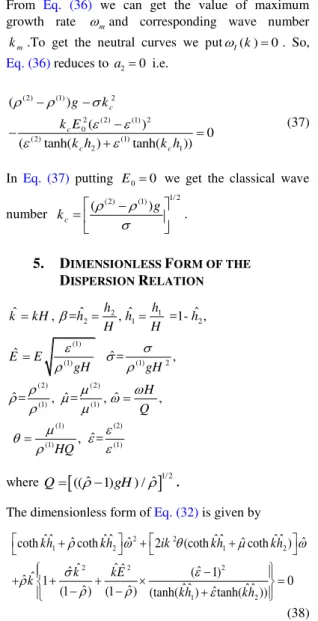
The variation of growth rate curves for different values of dielectric constant ratio of two fluids has been drawn in Fig. 4. It is observed that as the permittivity ratio of two fluids increases, growth of disturbance first increases and then decreases. This concludes that permittivity ratio has dual effect on the stability of the system.
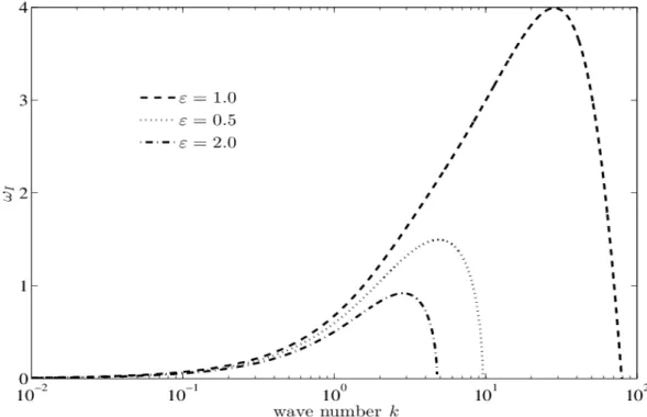
213 If electric field applied to the system in the tangential direction, fluids polarize in the direction of electric field and another electric force induces in the opposite direction of the applied electric field. In this situation electric field dominates not viscosity and so VPF solution and IPF solution gives almost same results but VPF solution still more stable due to viscous forces. We have computed the maximum growth rate for different values of electric field making other
parameters constant in the Table 1. It is observed that as electric field increases growth rate decreases i.e. electric field stabilizes the system. Table 2 compares the growth rates obtained for inviscid potential flow solution with the growth rates obtained in viscous potential flow solution. Growth rate for VPF solution is lower in comparison of IPF in the absence as well as in the presence of electric field as observed from the Table 2. So it is concluded that VPF solution is more stable in comparison with IPF solution.
Fig. 2. Neutral curves for Electric field when ˆ163.4721,ˆ.018,ˆ1.6882 for different values of upper fluid fraction
214
Fig. 4. Growth rate for VPF solution when ˆ0.018, ˆ163.4721, =0.5, =10 E for different values dielectric constant ratio
215
Fig. 6. Growth rate when ˆ0.018, ˆ163.4721, 0.5, E010volt cm/ for VPF and IPF solution
Table 1 Growth rate curves for ˆ0.018, ˆ163.4721, and ˆ1.6882, =0.5 for different values of electric
field
2 ˆ
h E0(volt/cm)
1
m( )
I
w s 1
m( )
k cm
0.5 0
5 10 15 20
3.9931 2.6616 1.4951 0.8120 0.2302
28.47 13.92 4.95 2.57 1.14
Table 2 Comparison of growth rate curves for ˆ0.018, ˆ163.4721, and ˆ1.6882, =0.5 for VPF and IPF solution for different values of electric field
2 ˆ
h E0(volt/cm) IPF solution VPF solution
0.5 0
5 10 15 20
5.4992 2.9580 1.5281 0.8208 0.2320
3.9931 2.6616 1.4951 0.8120 0.2302
7. CONCLUSION
Viscous potential flow analysis of Rayleigh-Taylor instability of two viscous, incompressible and dielectric fluids in the presence of tangential electric field has
216 stabilizing effect on the stability of the considered system while dielectric constant ratio plays dual role on the stability of the system. It has been also been observed that the viscous normal stresses stabilize the system.
REFERENCES
Asthana, R., M.K. Awasthi and G.S. Agrawal (2012). Viscous potential flow analysis of Rayleigh-Taylor instability of cylindrical interface. Applied Mechanics and Materials, 110-116, 769-775.
Awasthi, M.K. and G.S. Agrawal (2011). Viscous potential flow analysis of Kelvin-Helmholtz instability of cylindrical interface. Int. J. App. Math. Comp., 3, 131-138.
Awasthi, M.K. and G.S. Agrawal (2010). Viscous potential flow analysis of Rayleigh-Taylor instability with heat and mass transfer. Int. J. of Appl. Math. and Mech., 7, 1-12.
Chandrasekhar, S. (1981). Hydrodynamic and Hydromagnetic Stability. Dover publications, New York.
Dhananjay, G.S.A and R. Bhargava (2011). Rayleigh-Bénard convection in nanofluid. International Journal of Applied Mathematics and Mechanics, 7, 61-76.
Drazin, P.G and W.H. Reid (1981). Hydrodynamic Stability. Cambridge University Press, Cambridge.
Eldabe N.T. (1989). Effect of tangential electric field on Rayleigh-Taylor instability. J. Phy. Soc. Japan., 58, 115-120.
Joseph, D.D., G.S. Beavers and T. Funada (2002). Rayleigh-Taylor instability of viscoelastic drops at high Weber number. J. Fluid Mech., 453, 109-132. Joseph, D.D., J. Belanger and G.S. Beavers (1999). Breakup of a liquid drop suddenly exposed to high-speed airstream. Int. J. Multi. Flow, 25, 1263-1303.
Kumar, P. (2012). Thermosolutal magneto-rotatory convection in couple-stress fluid through porous medium. Journal of Applied Fluid Mechanics, 5, 45-52.
Lewis, D.J. (1950). The instability of liquid surfaces when accelerated in a direction perpendicular to their planes. Proc.R. Soc.London, Ser. A, 201, 81-96.
Mohamed, A.E.A., A.R.F. Elhefnawy and Y.D. Mahmoud (1993). Nonlinear electrohydrodynamic Rayleigh-Taylor instability with mass and heat transfer: Effect of a tangential field. Physica A, 195, 74-92.
Mohamed, A.M.A. and E. Shehawey (1983). Nonlinear electrohydrodynamic Rayleigh-Taylor instability Part 1: A perpendicular electric field in the absence of surface charge. J. Fluid. Mech., 129, 475-494.
Rayleigh, L. (1990). Scientific paper , Cambridge, U.P., Cambridge, Vol. II, pp. 200-207.
Rudraiah N. and G. Chandrashekara (2010). Effects of couple stress on the growth rate of Rayleigh- Taylor instability at the Interface in a finite thickness couple stress fluid. Journal of Applied Fluid Mechanics, 3, 83-89.
Taylor, G.I. (1950). The instability of liquid surfaces when accelerated in a direction perpendicular to their planes. Proc. R. Soc. London, Ser. A, 201, 192-196.
Yadav, D., G.S. Agrawal and R. Bhargava (2011). Thermal instability in rotating nanofluid. International Journal of Engineering Science, 49, 1171–1184.
Yadav, D., R. Bhargava and G.S. Agrawal (2012a). Boundary and internal heat source effects on the onset of Darcy-Brinkman convection in a porous layer saturated by nanofluid. International Journal of Thermal Sciences, 60, 244-254.
Yadav, D., G.S. Agrawal and R. Bhargava (2012b). The onset of convection in a binary nanofluid saturated porous layer. International Journal of Theoretical and Applied Multiscale Mechanics, 2, 198-224.
Yadav, D., G.S. Agrawal and R. Bhargava (2013a). The onset of double-diffusive convection in a layer of saturated porous medium with thermal conductivity and viscosity variation. Journal of Porous Media, 16, 105-121.
Yadav, D., R. Bhargava and G.S. Agrawal (2013b). Thermal instability in a nanofluid layer with vertical magnetic field. Journal of Engineering Mathematics. DOI 10.1007/s10665-012-9598-1.