Nonlinear wave interaction and resonance of spatially growing electrically forced jets

Journal homepage:www.ijaamm.com

International Journal of Advances in Applied Mathematics and Mechanics

Nonlinear wave interaction and resonance of spatially growing

electrically forced jets

Research Article

Saulo Orizagaa,∗, Daniel N. Riahib

a_{Department of Mathematics, Univesity of Arizona, 617 N. Santa Rita Ave, Tucson Arizona, 85735 USA}

b_{Department of Mathematics, University of Texas Rio Grande Valley, Brownsvville, Texas 78520 USA}

Received 13 September 2016; accepted (in revised version) 02 October 2016

Abstract: This paper considers the problem of nonlinear instability in electrically driven jets subject to spatially growing distur-bances in the presence of a uniform or non-uniform applied electric field. We use the original electro-hydrodynamic equations for mass conservation, momentum, charge conservation, and electric potential to model the viscous axis-symmetric jet flow. For the linear stage, a dispersion relation for this flow is derived and solved for two different types of fluids. We find that the lower viscosity fluid operates under the Rayleigh and conducting mode of instability. The higher viscosity fluid only operates under the conducting mode. We used those solutions from the dispersion rela-tion satisfying the resonance condirela-tion to study the nonlinear evolurela-tion of the problem. The dependent variables in the flow for the jet radius, jet’s velocity, jet’s electric field and jet’s surface charge are solved both in the linear and nonlinear formulation of the problem. The results are discussed and presented.

MSC: 76E30• 76E25

Keywords: Nonlinearity• Resonance wave interaction• Electric field

© 2016 The Author(s). This is an open access article under the CC BY-NC-ND license(https://creativecommons.org/licenses/by-nc-nd/3.0/).

1. Introduction

Electrically driven jets is an important, interesting and challenging problem in the area of physics, applied mathe-matics and fluid mechanics. The mathematical model describing the fluid flow in this system traces back to 1969 in the work published by Melcher and Taylor [1,2]. Even when this problem has been known for so long, most of the understanding of this problem lies at the linear stage of the flow. In 2001, there was a significant development in the theory of electrically driven jets in the work published by Hohman et al. [3,4]. The work in [3] extended the currently available understanding of electrically driven jets which at that time relied on very idealistic fluid flows in which a zero viscosity or infinite electrical conductivity was assumed. The work from Hohman et al. [3] resulted in a model that could analyze more realistic flows. Their work and efforts were concentrated at the linear temporal stage of problem. The main goal of this paper is to provide a study of electrically driven jets [5–9] at the nonlinear stage.

The governing equations we study here are applicable to various physical processes. Electrically driven jets have practical applications in the area of electrospraying [10] and electrospinning [3,4,9,11–14]. Electrospinning a tech-nology used to control and produce small fibers by the use of large electric fields. These fibers have applications that range from electrical circuits to bio-medical applications. Electrospinning has been known for many years but due to the complexity in the mathematical modeling this process is still conducted on a trial and error basis. This adds to our motivation to undertake this nonlinear problem.

∗ _{Corresponding author.}

This paper studies the nonlinear regime of electrically driven jets by considering nonlinear resonant two-wave in-teractions of spatially growing disturbances. The present study can be seen as an extension of the work done in [15] in which two-wave interactions of temporal instabilities were studied. However, we now consider instabilities that evolve in space. We find that such spatial instabilities subjected to dyad resonance conditions can be significantly stronger that corresponding temporal instability [15] of such modes and occur at a very short distance after the jet is emitted as seen in experiments [1,2,4]. For a more detailed introduction, we refer the reader to [15] . Other developments trace back to either space or time alone evolving instabilities [3,4,15,16] . The mathematical formulation at least as the main model equations (the system of four partial differential equations) remains the same but the nonlinear interactions explored here provides an entire new study in the jet flow system.

2. Mathematical model formulation

The mathematical modeling of the electrically driven jets is based on the governing electrohydrodynamic equa-tions [1,2] for the mass conservation, momentum, charge conservation and for the electric potential, which are given below

Dρ

D t +ρ∇ ·~u=0

ρD~u

D t = −∇P+ ∇ · ∇(µ~u)+q~E D q

D t + ∇ ·(KE~)=0

~

E= −∇_Φ

(1)

where D D t=

∂

∂t+~u·∇is the total derivative,~uis the velocity vector, P is the pressure,~Eis the electric field vector,Φis the electric potential, q is the free charge density,ρis the fluid density,µis dynamic viscosity,Kis electric conductivity andtis the time variable.

The modeling assumptions of an incompressible, axis-symmetric, and slender viscous jet and rescaling results in the non-dimensional equations for the electrically driven jets [15–17] gives

∂ ∂t(h

2₎₊ ∂ ∂z(h

2

v)=0 (2)

∂ ∂t(hσ)+

∂

∂z(hvσ)+

1 2

∂ ∂z(h

2

E K∗K˜(z))=0 (3)

∂v

∂t+v

∂v

∂z = −

∂ ∂z · h · 1+ µ ∂h ∂z

¶2¸−12 −∂

2_h ∂z2

· 1+

µ

∂h

∂z

¶2¸−32 −E

2

8π−4πσ 2¸

+ 2Eσ

hpβ

+3v ∗

h2

∂ ∂z(h

2∂v

∂z) (4)

Eb(z)=E−ln(X) ·

β

2

∂2 ∂z2(h

2_E)−4πq_β ∂ ∂z(hσ)

¸

(5)

where the dependent variables arev(z,t) is the axial velocity,h(z,t) is the radius of the jet cross-section at the axial locationz,σ(z,t) is the surface charge, andE(z,t) is the electric field. The conductivity K is assumed to be a function of z in the formK=_K0K˜(z), whereK0is a constant of dimensional conductivity and ˜K(z) is a non-dimensional variable

function,K∗=_K0©ρr₀3/[γβ(˜ǫ)2_]ª0.5

is the non-dimensional conductivity parameter,β=ǫ/˜ǫ−1,ν∗_=[ν2_ρ/(γr 0)]0.5

is the non-dimensional viscosity parameter,Eb(z) is an applied electric field and 1/Xis the local aspect ratio, which is assumed to be small. The above system admits the equilibrium solutionhb=1, vb=0, σb=σ0, Eb=Ω/ ˜K(z)=

Ω{ 1−δz} which has physical significance in the jet flow mechanism and provides a point for linearizing the system of partial differential equations given in Eq.3

HereΩandσ0are constant quantities. Hereσ0is the background free charge density. We setδ=8σ0π/(Ωp

β) to be a small parameter (δ<<1) and consider a series expansion in powers ofδfor all the dependent variables for the case of variable applied field. In this paper, we investigate the cases where applied electric field can be either uniform (δ=0) or non-uniform (δ6=0). This is related the electric field that is generated between the high voltage, which is applied at nozzle, and the distance from the nozzle to the grounded collector plate. This allows for perfect or imperfect alignment on the collector plate with respect to the nozzle orifice.

To formulate the problem of nonlinear resonance instability, we consider the solution to Eq. (3) to be a sum of the equilibrium solution plus a small perturbation.

whereh,v,σandEare the dependent variables for the perturbation quantities. We then use Eq. (6) in Eqs. (2)-(5) and keep linear terms on the left hand side and keep nonlinear terms in right hand side, which in vector notation reads

Lq=N (7)

whereq=(h,v,σ,E)T _{is the perturbation vector, and the linear operatorLand the nonlinear operatorNare given on} the Appendix. We now assume that the perturbation quantities are small and have the following form

( ˜h, ˜v, ˜σ, ˜E)=ǫ(h1,v1,σ1,E1)+ǫ2(h2,v2,σ2,E2) (8)

where the small parameterǫ (ǫ<<1)characterizes the magnitude of the disturbance quantity that causes pertur-bation. This parameter will play a very important role for the proper arrangement of the equations as well as the detection of the linear spatial instability modes that satisfy the resonance conditions.

2.1. Linear instability

For the linear case we keep only leading order terms in (8). We consider the following form for the perturbation quantities

(h1,v1,σ1,E1)=(h′,v′,σ′,E′)exp[iωt+(i+ks)z] (9)

which is constructed from plane waves that oscillate as well as grow or decay in the spatial direction. Using (9) in (7), we linearize with respect to the amplitude of perturbation and following [21] we arrive at the dispersion relation, which has the following form

1 4πp

β(4π(

q

βω¡

−i(k−i s)2¡

1+(k−i s)2−8πσ20

¢

+6(k−i s)2v∗ω+2iω2¢ −

8i K∗π(k−_{i s})3qβσ0Ω−2K∗(k−_{i s})2Ω2)+(k−_{i s})2qβ(4kπsβω(−1+2s2

+8πσ2₀−6i v∗ω)+2i k2πβω¡

−1+6s2+8πσ2₀−6i v∗ω¢

−8k2K∗π2

q

β(1−6s2

+8πσ2₀+6i v∗ω)+16i kK∗π2s

q

β¡

1−2s2+8πσ2₀+6i v∗ω¢

−2k4(4K∗π2

q

β

+iπβω)+8i k3(4K∗π2s

q

β+iπsβω)+8K∗π2

q

β(−s4+2ω2+s2(1+8πσ2₀

+6i v∗ω))−2iπω(32πσ20+β(s4−2ω2+s2(−1+8πσ2−6i v∗ω)))+64K∗π2

(i k+s)σ0Ω−(k−i s)2qβ³4K∗π+i

q

βω´Ω2)log[1/.89k])=0 (10)

The dispersion relation given by Eq. (10) is solved numerically for s andωnumerically using Newton’s method [15,16] .

2.2. Nonlinear instability

Here we investigate the effects of the nonlinear interactions of the modes that can satisfy dyad resonance condi-tions [18–22] on the nonlinear spatial instabilities of the jet. We introduce a slowly varying space variablezs=ǫz, we write the solution to the linear version of equation (7)

Lq1=0 (11)

q1≡(h1,v1,σ1,E1)⊤ (12)

in the following form

q1= 2

X

n=1

An(zs)q1nexp[i(knz+ωnt)+snz]+c.c (13)

q1n≡(h1n,v1n,σ1n,E1n)⊤ (14)

whereq1nis a vector with constant elements and c.c. denotes the complex conjugate of the preceding expression. We included in (13) terms due to two modes labeled as the mode 1 and the mode 2 with the corresponding amplitude functions An(zs)(n=1,2), wave numberskn(n=1,2), frequenciesωn(n=1,2) and small growth ratessn (sn =ǫs˜n with ˜sn of order one value or less) that satisfy the dyad resonance conditions in the sense thatk2=2k1andω2≈2ω1.

We refer to the resonance as a perfect resonance [18,19] ifω2=2ω1. For this investigation we have the wave number

whereµis an order one quantity and the so-called detuning parameter [23]ǫµrepresents a small deviation from perfect resonance. Using (13) in (11), we find

Lnq1n=0 (n=1,2) (15)

whereLn has the same form asL, provided (∂/∂z) and (∂/∂t) are replaced by (i kn+Sn)andiωn, respectively. Using (8), (11)-(14) in (7), we find that in the orderǫ2the following nonlinear equation becomes

Lq2=N1 (16)

q2≡(h2,v2,σ2,E2)⊤ (17)

where the expression for the nonlinear operatorN1is given in the Appendix. The solution to (16)-(17) has the following

form

q2= 2

X

n=1

q2nexp[i(knz+ωnt)+snz]+c.c (18)

q2n≡(h2n,v2n,σ2n,E2n)⊤ (19)

where the vectorq2nis a function ofzs. Using (18) in (16), we find

Lnq2n=N1n (n=1,2) (20)

where the expressions for the vectorsN1n(n=1,2) are are given in the Appendix. The governing equations for the amplitude functionsAn(zs) will derive from the solvability condition or Fredholm alternative [18,24] for the Eq. (20). Here we briefly provide the general idea of the solvability condition.

Using the solvability condition, defines the adjoint solutionq(₁a_n)by the property [18,24]

(Lnq1n,q(₁a_n))=(q1n,L(na)q(1an)), (n=1,2) (21) q(₁a_n)≡(h₁(a_n),v₁(a_n),σ₁(a_n),E₁(a_n))⊤ ₍₂₂₎

Here we denote the usual inner product (x,y)=_x⊤_y∗, where â ˘AŸ∗_{â ˘A´Z is used for the complex conjugate. Eqs.} (21)-(22) follow since (15) is the related linear problem of (20). HereLn(a)is the linear adjoint operator, andq(1an)is the solution vector to the homogeneous adjoint problem, which represents the null space of the adjoint operatorL(na). Taking inner product of (15) withq(₁a_n)and using (21)-(22), we look for non-trivial solution of the adjoint system

L_n(a)q(₁a_n)=0, (n=1,2) (23)

whereL(na)is a 4 by 4 matrix differential operator, which is given in the Appendix. Taking inner product of (20) with the adjoint solutionq(₁a_n)found from Eq. (23) and making use of the property (21), we arrive at the solvability conditions for Eq. (20) for bothn=1,2.

(N(₁a_n),q₁(a_n))=0, (n=1,2) (24)

Each of this n values will produce a lengthy ordinary differential equations. The system of nonlinear differential equations contains complex conjugate of the amplitude functions, complex coefficients and exponential components that have the corresponding spatial growth rates of the resonant modes we found earlier. The two differential equa-tions that govern the slowly varying amplitudes funcequa-tionsA1(zs) andA2(zs), which are modulated by the nonlinear wave interactions, have the following form

c1d A1(zs)

d zs

+_c2A1(zs)∗A2(zs)exp[iǫµt+s2z]=0 (25)

d1d A2(zs)

d zs

+_d2A2(zs)+d3A1(zs)2exp[(2s1−s2)z−iǫµt]=0 (26)

where′_∗′_{indicates complex conjugate and the expressions for the constant complex coefficientsc}

n(n=1,2), and

dm(m=1,2,3) are given in the Appendix. The solutions to Eqs. (25)-(26) forA1and A2versus spatial variable are

3. Results and discussion

The results we provide here are the linear and nonlinear instability in electrically driven jets. The linear results are obtained from the solution of the dispersion relation given by Eq.(10). To study the nonlinear evolution of the problem, we find solutions to Eq. (10) that satisfy the two-wave interaction (resonance conditions) and used those solutions to solve the system of differential equations governing the amplitude functions A1 andA2, which are the solutions to Eqs. (25)-(26). Using the amplitude functionsA1,A2 in Eqs. (13)-(14) provides the nonlinear evolution of the problem with respect to spatially growing disturbances. These are the perturbation quantities and nonlinear solutions to the problem. We will compare the perturbation quantities in absence of nonlinear wave interactions (linear perturbation quantities) and nonlinear solutions (in presence of nonlinear wave interactions). In the results we provide, we include two fluids of practical relevance water-glycerol mixture and glycerol. Parameter values areK∗_=19.60,ν∗_(glycerol) =9.05384,ν∗_{(water-glycerol)=0.60764, andβ=77. In addition,ǫ=0.01,σ0=0 for the uniform applied field , and}

σ0=0.10. for the nonuniform applied field.Ω=1,3 was used for the intensity of the applied electric field. Our main results are presented in the following subsections.

3.1. Water-glycerol mixture jet

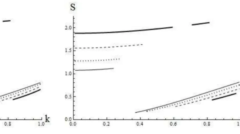
Figs. 1and2represent the growth rate s versus the axial wave number k for the non-uniform applied field (σ0=0.1) and the uniform applied field (σ0=0), respectively, and for different values ofΩ. It can be seen from theFig. 1that the growth rate s are divided into two main branches and in the case whereΩ=4 there is even a third branch for the growth rates s, in particular, when we consider the uniform applied field. For the branch containing the lower range wave numbers, we can detect that the instabilities grow in moderate magnitude as the wave number is increased, but we can see significant instability growth by incrementing the magnitude of theΩ. This instability is referred as conducting type of instability [3]. We can also observe that the range of values for the wave number increases for larger values ofΩ. From the higher wave number values onFig. 1, which is the other solution branch, we detect the similar effect as for the low wave numbers in the sense that s increases as k increases, but now at a higher rate. This solution branch for the spatial growth rate becomes more stable for higher values ofΩ, which is the classical Rayleigh type of instability and at the same time the wave number range where these modes operate gets reduced. InFig. 2, we have the same representation asFig. 1, but now for (σ0=0). The results obtained from this figure indicate that uniform applied field provides stabilization since all modes of instability were reduced compared to non-uniform variable applied field (σ0=0.1). ForΩ=3, we found the modes of instability that satisfy the dyad resonance conditions for non-uniform

Fig. 1.The growth rate s versus the axial wave number k and for water-glycerol mixture jet withΩ=1 (thin solid line), 2 (dotted line), 3 (dashed line) and 4 (thick solid line) and for variable applied field (σ0=0.1).

Fig. 2.The same as in theFig. 1but for constant applied field (σ0=0).

applied field whereσ0=0.1.Figs. 3and4present results for the dependent variables of the perturbation versuszfor

t=1,k1=0.1,k2=0.2,ω1=0.09488,ω2=0.19131,s1=1.68026 ands2=1.68949. The initial conditions chosen for the

amplitude functions wereA10=0.1+0.1iandA20= −0.1+0.1i. It can be seen from the results presented in theFig. 3

Fig. 3.Perturbation quantities h1 (thin solid line), v1 (dotted line),σ1(dashed line) and E1 (thick solid line)

versus the axial variable z for water-glycerol jet and for the two modes 1 and 2 that satisfy the dyad resonant

conditions. Hereσ0=0.1,t=1,k1=0.1,k2=0.2,ω1= 0.09488,ω2=0.19131,s1=1.68026 ands2=1.68949 and

Ω=3.and nonlinear mode interactions are fully taken into account.

Fig. 4.The same as in theFig. 3but in the absence of nonlinear interactions.

3.2. Glycerol jet

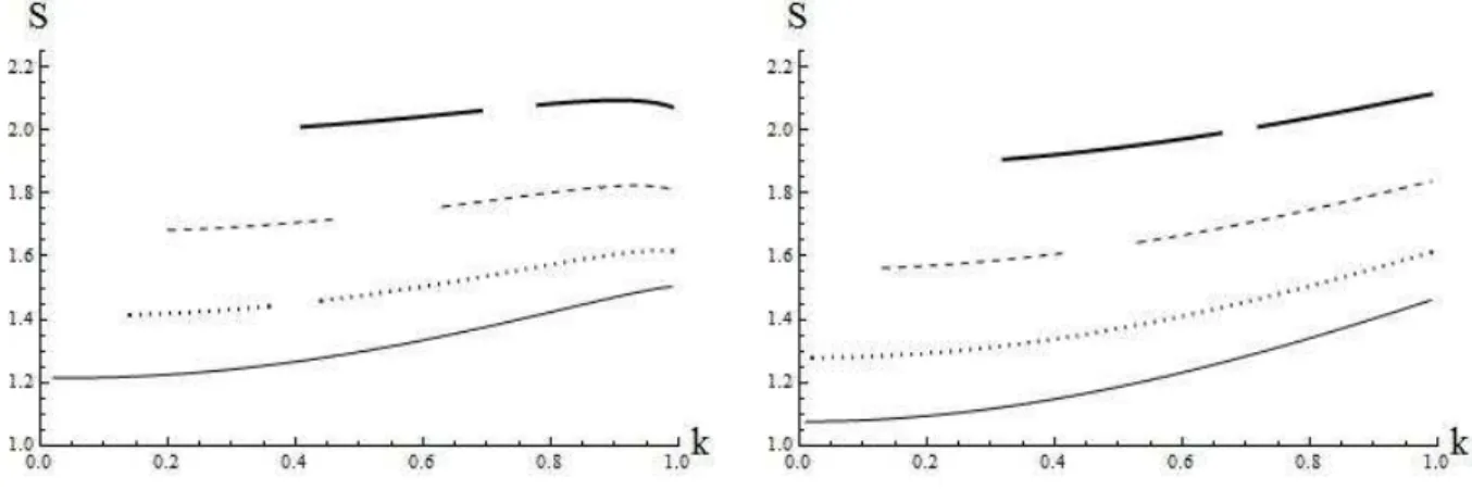
Figs. 5 and6present the growth rate s versus the axial wave number for the non-uniform applied field, where

σ0=0.1, and the uniform applied field, whereσ0=0, respectively, and for different values ofΩ. It can be seen from these figures that growth rate s undergoes a similar branching process, but for these cases under this higher viscosity from glycerol these two modes seem to carry similar properties. The properties include in either case of 1 mode or 2 modes depending onΩ, the modes increase as k increases and all these modes are enhanced as the magnitude of the electric field is intensified, which refers to the conducting mode of instability. HereΩis strictly destabilizing for the spatial growth rates s. The uniform applied field provides a slightly advantage in the sense of stability compared to the non-uniform applied field. For the case forσ0=0.1, the simulations detected slightly stronger type of instabilities. ForΩ=1, we found modes that satisfy the dyad resonance conditions for non-uniform applied field whereσ0=0.1.

Fig. 5.The same as in theFig. 1but for glycerol jet. Fig. 6.The same as in theFig. 2but for glycerol jet.

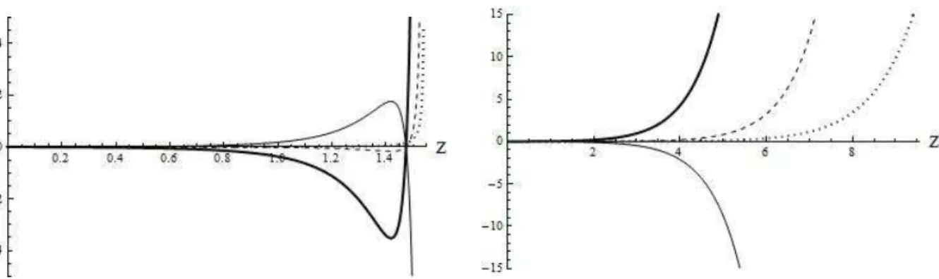
Figs. 7s and8present results for the dependent variables of the perturbation versus z in the presence of the nonlinear mode interactions (Fig. 7) and in the absence of such interactions (Fig. 8) and fort=1,k1=0.07,k2=0.14,ω1=

0.00319,ω2=0.00639,s1=1.21478 ands2=1.21859. The initial conditions for the amplitude functions wereA10=

A20=0.1+0.1i. It can be seen from the results presented in these figures that the amplitudes of the perturbation

Fig. 7.The same as in theFig. 3but for σ0=0.1,Ω=1,t=1,k1=0.07,k2=0.14,ω1= 0.00319,ω2=0.00639,s1=1.21478 ands2=1.21859.

Fig. 8.The same as in theFig. 7but in the absence of nonlinear interactions.

4. Conclusion

We studied the problem of nonlinear spatial instability in electrically driven viscous jets under a uniform and nonuniform applied electric field. We derived the dispersion relation for the case of glycerol and water-glycerol fluid flows. At the linear stage, we find that the glycerol jet exhibits the conducting type of instability which is driven by the applied electric field. The water-glycerol mixture exhibits two modes of instabilities corresponding to the conducting type and the other to the classical Rayleigh instability. At the nonlinear state, the nonlinear wave interactions under the resonance conditions were able to provide very distinct evolution in the perturbation plots, which included jet radius decreasing at a higher rate and at a shorter axial location. The nonlinear investigation provides new operating regimes very different from classical linear theory. Under resonance, the instabilities are intensified and the jet radius is significantly reduced which is a mechanism of interest in applications such as electrospinning. This suggests that under the studied nonlinear approach, practical applications to electrically driven jets could benefit by controlling the jet flow instabilities to produce higher quality jet fiber that are smaller in size.

For near future research, we plan to investigate resonant nonlinear wave interactions of three-modes (triads) for the case of space and time evolving instabilities. In addition, we intend to extend the analysis done here to consider other types of flows. Hydromagnetic flows in thin films [25-27] have gained a lot of attention recently among scientists due to the large number of applications they have and understanding this problem at the nonlinear stage becomes a natural choice for our future research.

Acknowledgements

S.O. was supported through a NSF-Alliance Postdoctoral Award DMS-0946431

Appendix

The expressions for the 4 by 4 matrix operatorLand the vector operatorNare given below

L=(r ow1,r ow2,r ow3,r ow4)⊤ (A.1a)

where ther owi(i=1,2,3,4) is thei t hrow of the matrix operatorLgiven by

r ow1=[2∂ ∂t,

∂ ∂z,0,0] r ow2=[(σ0∂

∂t+ΩK

∗ ∂

∂z),σ0

∂ ∂z,

∂ ∂t,

1 2K

∗ ∂

∂z( ˜K(z))] (A.1b)

r ow3=[( ∂ ∂z−

∂3 ∂z3),(

∂ ∂t−3ν

∗ ∂2

∂z2),(−8πσ0 ∂ ∂z−

2 p

βEb),(−

1 4π

∂ ∂zEb−

2 p

β σ0)]

r ow4=[(−βln(X) ∂ 2

∂z2(vEb)+4π

q

βσ0∂

∂z),0,(4ln(X)π

q

β ∂ ∂z),(1−

1 2ln(X)

β∂ 2

N=(el em1,el em2,el em3,el em4)⊤ (A.2a)

whereel emi(i=1,2,3,4) are the entries of the nonlinear oepratorNgiven by

el em1= −[∂ ∂th

2₊₂ ∂ ∂z(hv)] el em2= −[∂

∂t(σh)+(σ0

∂ ∂z(vh)+

∂ ∂z(vσ)+

1 2K

∗ ∂

∂z(2 ˜K(z)E h+Ωh

2_)]

el em3=[−v∂v ∂z −

∂ ∂z(

1 2 µ ∂h ∂z ¶2 −1 8E

2_−4πσ2₎₊ 2

p

β(Ebh

2_{+Eσ−σ0E h−}

Ebhσ)+3ν∗

∂ ∂z(2h

∂v

∂z)+3ν

∗₍₋₂

h) ∂

∂z(

∂v

∂z+2h

∂v

∂z)]

el em4=ln(X)[β

2

∂2 ∂z2(Ebh

2₊₂

hE)− 4π p

β ∂

∂z(hσ)] (A.2b)

The expression for the elements of the nonlinear operatorN1are given below

N1=(el em1,el em2,el em3,el em4)⊤ (A.3a)

whereel emi(i=1,2,3,4) are the entries of the nonlinear oepratorN1given by

el em1= −2[h1∂h1 ∂t +h1

∂v1 ∂z +v1

∂h1 ∂z +

∂v1 ∂zs

] (A.3b)

el em2=σ1∂h1 ∂t +h1

∂σ1 ∂t +σ0v1

∂h1 ∂z +σ0h1

∂v1 ∂z +σ1

∂v1 ∂z +v1

∂σ1 ∂z +

1 2K

∗ ∂

∂z

(2E1h1+Ωh21)−σ0 ∂v1 ∂zs

−1 2K

∗ ∂

∂zs

(E1+2Ωh1)

el em3= −v1∂v1 ∂z +

1 2

∂ ∂z

µ

∂h1 ∂z

¶2 + 1

4πE1 ∂E1

∂z +8πσ1

∂σ1 ∂z +

2 p

β(Ωσ0h 2 1−Ωσ1

h1−σ0E1h1−σ1E1)6ν∗ ∂ ∂z(h1

∂v1 ∂z )−6ν

∗

h1∂ 2_v

1 ∂z2 −

∂h1 ∂zs

+3( ∂

2

∂z2

∂ ∂zs

)

h1+ Ω

4π ∂E1

∂zs

+8πσ0∂σ1 ∂zs

+6ν∗( ∂

∂z

∂ ∂zs

)v1

el em4=ln(X)[β

2

∂2 ∂z2(Ωh

2

1+2h1E1)−4π

q

β ∂

∂z(h1σ1)]+ln(X)[

β

2

∂2 ∂z2s

(2Ωh1

+_E1)−4π

q

β ∂ ∂zs

(σ1+_σ0h1)]

The expressions for the elements of the vectorsN11andN12are given below

N11=(el em1,el em2,el em3,el em4)⊤ (A.4a)

whereel emi(i=1,2,3,4) are the entries of the nonlinear oepratorN11given by

el em1= −v11d A1

(zs)

d zs

+((i k1+s1+s2)v12+i h12(ǫµ+ω1))h∗11+h12(i k1+s1

+s2)v11∗)A1(zs)∗A2(zs)exp[iǫµt+s2z] (A.4b)

el em2=(−K

∗

2 E11−v11σ0−h11K ∗

Ω)d A1(zs)

d zs

+(h12K∗(i k1+s1+s2)E11∗+

((i k1+s1+s2)(E12K+v12σ0+h12K∗Ω)+iσ12(ǫµ+ω1))h11∗ +(i k1

+_s1+_s2)(h12σ0+σ12)v∗11+((i k1+s1+s2)v12+i h12(ǫµ+ω1))σ∗11)

A1(zs)∗A2(zs)exp[iǫµt+s2z]

el em3=(3(i k1+s1)2−1)h11+8πσ0σ11+6ν∗(i k1+s1)v11+ Ω

4πE11)

d A1(zs)

d zs

+ 1 4πp

β[(E12(i k1

+_s1+_s2)qβ+8π(σ12−σ0h12)E∗114π(k1+i s1)

(2k1+i s2)(h12(i k1+s1+s2)+6ν∗v12)

q

σ12Ω)h₁₁∗6h12ν∗(k1+i s1(2k1+i s2)−(i k1+s2+s2)v12)

q

βv₁₁∗ +2(

E12+4π(i k1+s2+s2)

q

βσ12−_Ωh12σ∗11)A1(zs)∗A2(zs)exp[iǫµt+s2z]

el em4=(1

2β(E11+2h11Ω)ln(X))

d2A1(zs)

d z2s

−(4π

q

β(σ0h11+σ11)ln(X))d A1(zs)

d zs

+[qβ(k1−i(s1+s2))ln(X)(h12(k1−i(s1+s2))

q

βE11∗ +(4iπσ12+

(k1−i(s1+s2))

q

β(E12+h12Ω))h∗11+4iπh12σ∗11]A1(zs)∗A2(zs) exp[iǫµt+s2z]

N12=(el em1,el em2,el em3,el em4)⊤ (A.5a)

whereel emi(i=1,2,3,4) are the entries of the nonlinear oepratorN12given by

el em1= −v12d A2(zs)

d zs

−2i[h11(2k1v11−2i s1v11+h11ω11]A1(zs)2exp[(2s1−s2)

z−_iǫµt]

el em2= −(K

∗

2 E12+σ0v12+h12K ∗

Ω)d A2(zs)

d zs

−[(i k1+s1)(K∗h11E11+2v11(

σ0h11+σ11+2i h11σ11ω1]A1(zs)2exp[(2s1−s2)z−iǫµt] (A.5b)

el em3= 1

4π[4π−(1+3(2k1−i s1) 2₎

h12+6(8πσ0σ12+ν∗(2i k1+s2)v12)+Ω

E12]d A2

(zs)

d zs

+ 1 4πp

β[(E 2

11(i k1+s1)

q

β+8π(σ11−σ0h11))E114π(i k1

+_s1)qβ(−_h112(k1−i s1)2+6h11ν∗(i k1+s1)v11−v112 +8σ211)+8πh11

Ω(σ0h11−σ11)]A(zs)2exp[(2s1−s2)z−iǫµt]

el em4=(1

2β(E12+2h12Ω)ln(X))

d2A2(zs)

d z2s

−(4π

q

β(σ0h12+σ12)ln(X))d A2(zs)

d zs

+[2h11

q

β(i ki+s1)ln(X)(−4πσ11+(i k1+s1)

q

β(2E11+h11Ω)))]

A1(zs)2exp[(2s1−s2)z−iǫµt]

The expressions for the 4 by 4 matrix differential operatorL(na)is given below

L(na)=(r own1,r own2,r own3,r own4)⊤,(n=1,2), (A.6a)

wherer owni(i=1,2,3,4) is thei t hrow of the matrixL(na)and given by

r own1=[−2iωn,−σ0iωn+K∗Ω(−kn+sn),(kn+i sn)(kn+i sn+i)(sn−i kn

−1)+ 2 p

βΩσ0,ln(

X_)(kn+i sn)(−4iπσ0(kn+i sn) q

βΩ)]

r own2=[sn+i kn,σ0(sn−i kn),3(kn+i sn)2ν∗−iω1,0] (A.6b)

r own3=[0,−iω1,−(8πσ0(sn−i kn)+ 2 p

βΩ),−4π

q

β(kn+i sn)ln(X)]

r own4=[0,

1 2K

∗₍

sn+i kn),−( 2 p

βσ0+

2

4πΩ(sn−i kn)),1+(kn+i sn) 2_ln(X)

β]

The expressions for the coefficientscn(n=1,2,3) anddm(m=1,2,3,4) are given below

c1= −v11h(₁₁a)+(−K

∗

2 E11−v11σ0−h11K ∗

Ω)v₁₁(a)+(3(i k1+s1)2−1)h11+8π

σ0σ11+6ν∗(i k1+s1)v11+ Ω

4πE11)σ (a) 11−(4π

q

c2=((i k1+s1+s2)v12+i h12(ǫµ+ω1))h∗11+h12(i k1+s1+s2)v11∗)h(11a)+

(h12K∗(i k1+s1+s2)E11∗ +((i k1+s1+s2)(E12K+v12σ0+h12K∗Ω)+i σ12(ǫµ+_ω1))h∗11+(i k1+s1+s2)(h12σ0+σ12)v∗11+((i k1+s1+s2)v12+i h12

(ǫµ+ω1))σ∗₁₁)v(₁₁a)+ 1

4πpβ[(E12(i k1

+s1+s2)

q

β+8π(σ12−σ0h12)E11∗4π(k1

+i s1)(2k1+i s2)(h12(i k1+s1+s2)+6ν∗v12)

q

β−2E12σ0+4h12σ0Ω−2σ12Ω)

h∗116h12ν∗(k1+i s1)(2k1+i s2)−(i k1+s2+s2)v12)

q

βv∗11+2(E12+4π(i k1+s1

+_s2)qβσ12−_Ωh12σ∗₁₁)]σ(₁₁a)+[qβ(k1−i(s1+s2))ln(X)(h12(k1−i(s1+s2))

q

βE∗₁₁+(4iπσ12+(k1−i(s1+s2))

q

β(E12+h12Ω))h11∗ +4iπh12σ∗11]E11(a) (A.7b)

d1= −v12h(₁₂a)−(K

∗

2 E12+σ0v12+h12K ∗

Ω)v₁₂(a)+h12

4π(4π−(1+3(2k1i s1) 2₎

+6(8πσ0σ12+ν∗(2i k1+s2)v12)+ΩE12]σ(₁₂a)−(4π

q

β(σ0h12+σ12)ln(X))E(₁₂a) (A.7c)

d2= −2iµh12h₁₂(a)−(iµσ12+iµσ0h12)v₁₂(a)−iµv12σ(₁₂a) (A.7d)

d3= −2i[h11(2k1v11−2i s1v11+h11ω11]h12(a)+ −[(i k1+s1)(K∗h11E11+2v11(σ0

h11+σ11+2i h11σ11ω1]v₁₂(a)+ 1

4πp

β[(E 2

11(i k1+s1)

q

β+8π(σ11−_σ0h11))E11

4π(i k1+s1)

q

β(−h2₁₁(k1−i s1)2+6h11ν∗(i k1+s1)v11−v112 +8σ211)+πh11Ω

(σ0h11−σ11)]σ(₁₂a)+[2h11

q

β(i ki+s1)ln(X)(−4πσ11+(i k1+s1)

q

β(2E11

+_h11Ω))]E₁₂(a) (A.7e)

References

[1] G.I. Taylor, Electrically driven jets, Proc. Royal Soc. London, Series A. 313 (1969) 453–475.

[2] J.R. Melcher and G. I. Taylor, Electro-hydrodynamics: A review of the interfacial shear stresses, Annual Rev. Fluid Mech. 1 (1969) 111–146.

[3] M.M. Hohman, M. Shin, G. Rutledge, M. P. Brenner, 2001a, Electrospinning and electrically forced jets. I. Stability theory, Phys. of Fluids 13(8) (2001) 2201–2220.

[4] M.M. Hohman, M. Shin, G. Rutledge, M. P. Brenner, 2001b, Electrospinning and electrically forced jets. II. Appli-cations, Phys. of Fluids 13(8) (2001) 2221–2236.

[5] H. Schlichting, Boundary Layer Theory, seventh ed., McGraw-Hill, New York. 1979.

[6] V.Y. Shkadov, A.A. Shutov, Disintegration of a charged viscous jet in a high electric field, Fluid Dyn. Res. 28 (2001) 23–29.

[7] C.K.W. Tam, A.T. Thies, Instability of rectangular jet, J. Fluid Mech. 248 (1993) 425–448.

[8] J.J. Healey, Inviscid axisymmetric absolute instability of swirling jets , J. Fluid Mech. 613 (2008) 1–33. [9] A. Michalke, On spatially growing disturbances in an inviscid shear layer, J. Fluid Mech. 23 (1965) 521–544. [10] A.G. Baily, Electro-Static Spraying of Liquid, Wiley, New York. 1998.

[11] D.H. Reneker, A.L. Yarin, H. Fong, Bending instability of electrically charged liquid jets of polymer solutions in electrospinning, J. Applied Phys. 87 (2000) 4531–4547.

[12] D. Li, Y. Xia, Direct fabrication of composite and ceramic hollow nanofibers by electrospinning, Nano. Lett. 4 (2004) 933–938.

[13] J.H. Yu, S.V. Fridrikh, G.C. Rutledge, Production of sub-micrometer diameter fibers by two-fluid electrospinning, Advanced Materials 16 (2004) 1562–1566.

[14] D.L. Soderberg, Absolute and convective instability of a relaxational plane liquid jet, J. Fluid Mech. 439 (2003) 89–119.

[16] S. Orizaga, D.N. Riahi, Spatial instability of electrically driven jets with finite conductivity and under constant or variable applied field, Applications and Applied Math.: An Int. J. 4(2) (2009) 249–262.

[17] D.N. Riahi, On spatial instability of electrically forced axisymmetric jets with variable applied field, Appl. Math. Modeling 33 (2009) 3546–3552.

[18] N. Rott, A multiple pendulum for the demonstration of non-linear coupling, Z. Angew. Math. Phys. 21 (1970) 570–582.

[19] P.G. Drazin, W.H. Reid, Hydrodynamic Stability, Cambridge University Press, UK. 1981.

[20] A.D.D. Craik, Nonlinear resonant instability in boundary layers ,J. Fluid Mech. 50 (1971) 393–413.

[21] M.P. Vonderwell, D.N. Riahi, Resonant instability mode triads in the compressible boundary layer flow over a swept wing , Int. J. Engr. Sci. 36 (1998) 599–624.

[22] A. D. D. Craik, Wave Interactions and Fluid Flows, Cambridge University Press, UK. 1985.

[23] N.M. El-Hady, Evolution of resonant wave triads in three-dimensional boundary layers, Physics of Fluids A 1 (1989) 549–561.

[24] I. Stakgold, Green’s Functions and Boundary Value Problems, second ed.,Wiley, New York. 1998.

[25] M.S. Abela, P.G. Metri, Hydromagnetic flow of a thin nanoliquid film over an unsteady stretching sheet, Int. J. Adv. Appl. Math. and Mech. 3(4) (2016) 121–134.

[26] V.G. Gupta, A. Jain, Back flow analysis of unsteady MHD fluid flow over stretching surface with Hall Effect in presence of permeability,Int. J. Adv. Appl. Math. and Mech. 3(4) (2016) 102–113.

[27] J. Tawade, M.S. Abel, P.G. Metri, A. Koti ,Thin film flow and heat transfer over an unsteady stretching sheet with thermal radiation, internal heating in presence of external magnetic field,Int. J. Adv. Appl. Math. and Mech. 3(4) (2016) 29–40.

Submit your manuscript to IJAAMM and benefit from:

◮ Rigorous peer review

◮ Immediate publication on acceptance

◮ Open access: Articles freely available online

◮ High visibility within the field

◮ Retaining the copyright to your article