WAVELET TRANSFORMS IN TIME SERIES ANALYSIS

R.C. SINGH

Abstract

The existing methods based on statistical techniques for long range forecasts of Indian summer monsoon rainfall have shown reasonably accurate performance, for past 10 years. Because of the limitation of such statistical techniques, new techniques may have to be tried to obtain better results. Time series analysis and forecasting using wavelet transforms has become a powerful tool to determine, within a time series, both the dominant modes of variability and how those modes vary in time. A preliminary investigation, using wavelet analysis, on temperature and rainfall time series is presented.

1. TIME SERIES ANALYSIS

A time-series is a collection of observations made sequentially through time. Some examples are given as below:

฀ Sales of a particular product in successive months,

฀ Temperature at particular location at noon on successive days, and

฀ Electricity consumption in a particular area for successive one-hour periods.

62

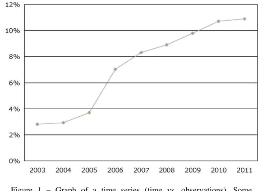
Figure 1 – Graph of a time series (time vs. observations), Some common examples of time – series

ECONOMIC TIME-SERIES: Time series that occurs in economics such as

฀ Share prices on successive days

฀ Export totals in successive months

฀ Average incomes in successive months

63

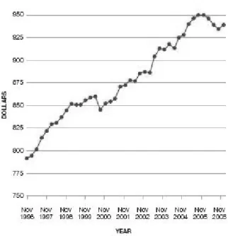
Figure 2- Some common examples of time – series

PHYSICAL TIME-SERIES: Time series that occurs in the physical sciences, particularly in meteorology, marine science, and geophysics;

฀ Rainfall on successive days,

64

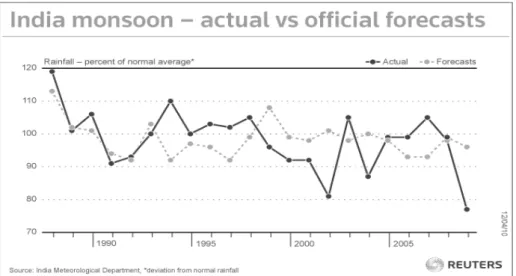
Figure 3- Rainfall, percent of normal average.

MARKETING TIME-SERIES:

฀ Sales figures in successive weeks or months,

65

Figure 4- Annual attrition rates

DEMOGRAPHIC TIME-SERIES:

฀ Time series that occurs in the study of population

66

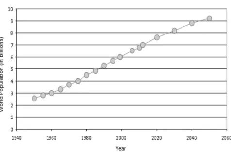
Figure 5- Annual variation of global population

PROCESS CONTROL: In process control, the problem is to detect changes in the performance of a manufacturing process by measuring a variable which shows the quality of the process.

BINARY PROCESS: A special type of time series arises when observations can take only two values, usually denoted by 0 and 1. Time series of this type, called binary processes, occurs particularly in communication theory.

67

POINT PROCESSES:

฀ Time series that occurs when a series of events occurring ‘randomly’ in time is Considered,

฀ Record the dates of major railway disasters.

Figure 6- Significant UK train accidents per million train km (5 year Rolling average).

฀ A series of events of this type is often called a point process. For observations of this type, the distribution of the number of events occurring in a given time-period and also in the distribution of time intervals between events is considered.

TYPES OF TIME – SERIES: 1. Continuous Time - Series

2. Discrete Time – Series

CONTINUOUS TIME SERIES

฀ A time series is said to be continuous when observations are made continuously in time.

68

฀ The usual method of analyzing such a series is to sample (or digitize) the series at equal intervals of time to five a discrete time series. Little or no information is lost by this process provided that the sampling interval is small enough.

GRAPH OF CONTINUOUS TIME SERIES:

฀A time series is said to be discrete when observations are taken only at specific times, usually equally spaced. Discrete Time Series may arise in three distinct ways:

฀By being sampled from a continuous series (e.g. temperature measured at hourly intervals.

฀By being aggregated over a period of time (e.g. total sales in successive months and rainfall measured daily)

฀As an inherently discrete series (e.g. the dividend paid by a company in successive years, Financial Times share index at closing time on successive days).

DISCRETE TIME SERIES

The special feature of time series analysis is the fact that successive observations are usually not independent and that the analysis must take into account the time order of the observations. When successive observations are dependent, future values may be predicted from past observations. If a time series can be predicted exactly, it is said to be deterministic. But most time series are stochastic in that the future is only partly determined by past values. For stochastic series exact predictions are impossible and must be replaced by the idea that future values have probability distribution which is conditioned by knowledge of past values.

OBJECTIVES OF TIME SERIES ANALYSIS:

DESCRIPTION

69

EXPLANATION/MODELLING

When observations are taken on two or more variables, it may be possible to use the variation in one time series to explain the variation in another series. This may lead to a deeper understanding of the mechanism which generated a give time series.

PREDICTION/FORECASTING

Given an observed time series, one may want to predict the future values of the series.

This is an important task in sales forecasting, and in the analysis of economic and industrial time series.

CONTROL

When a time series is generated this measures the ‘quality’ of a manufacturing

2. WAVELET TRANSFORMS

WAVE AND WAVELET: WAVE

฀ An oscillating function of time or space

Figure 7- Sine Wave

70

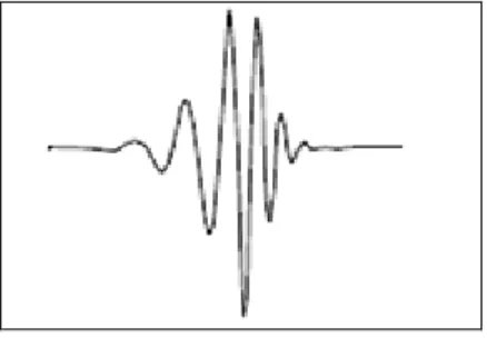
WAVELET

฀ Small wave which oscillates and decays in the time domain,

฀ Small wave which has its energy concentrated in time,

฀ Waveform of effectively limited duration that has an average value of zero.

Figure 8- Wavelet

Properties of Wavelets: A function to be a wavelet must satisfy:

 The wavelet must be centered at zero amplitude

(1)

 The wavelet must have a finite energy. Therefore it is localized in time (or space)

(2)

 Sufficient condition for inverse wavelet transforms

(3)

Popular wavelets which satisfy the previous conditions:

∫

=

0

)

(

t

dt

ψ

∞

<

∫

dt

t

)

|

71

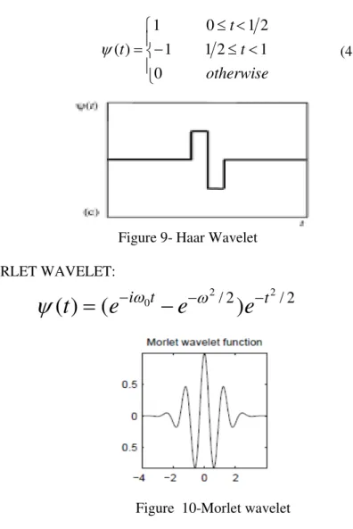
HAAR WAVELET:

 The first wavelet introduced in 1909

(4)

Figure 9- Haar Wavelet

MORLET WAVELET:

(5)

Figure 10-Morlet wavelet











<

≤

−

<

≤

=

otherwise

t

t

t

0

1

2

1

1

2

1

0

1

)

(

ψ

2

/

2

/

)

(

)

(

i

t

t

e

e

e

t

=

−

ω

−

−

ω

−

72

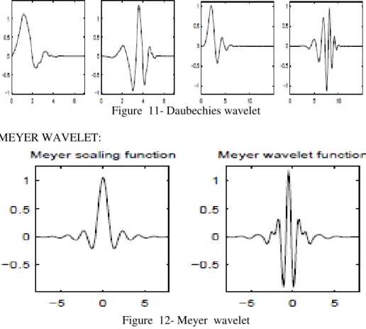
Morlet wavelet can be considered as a modulated Gaussian waveform DAUBECHIES WAVELET:

Figure 11- Daubechies wavelet

MEYER WAVELET:

73

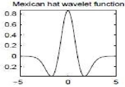
MEXICAN HAT WAVELET:

Figure 13-Mexican wavelet

 Useful for detection in computer vision.

 It is the second derivative of a Gaussian function. .

 The Mexican hat wavelet is defined:

(6)

Fourier Analysis:

 Excellent tool for analyzing periodic signals (sine and cosine signals)

 The Fourier transform of a function f(t) is given by

(7)

 The original function can be recovered from the transform using

(8)

2 2

₎

1

(

)

(

e

t

t

=

−

ψ

∫

−

=

f

t

e

dt

f

ˆ

(

ω

)

(

)

ω

ω

d

e

f

t

f

∫

∞ −

=

ˆ

(

)

)

74

 Transforms a function from time domain to frequency domain.

 Inefficient for representing transient signals.

Figure 14- Fourier Transform

Examples: (Music, image, speech, acoustic noise, seismic signals, thunder, and lightning, etc.)

Drawbacks:

 The Fourier Transform can be computed for only one frequency at a time.

 Exact representations cannot be computed in real time.

 The Fourier transform provides information only in the frequency domain, but not in the time domain.

Short-time Fourier Transform (STFT) / Windowed Fourier Transform:

 Introduced by Gabor in 1946

 Used to gain information from both time and frequency domains simultaneously

 The STFT is formally defined by the integral transform

(9)

∫

−

−

=

f

t

w

t

e

dt

f

75

Figure 15- Short Time Fourier Transform

Disadvantages of STFT:

 The size of the time window once chosen can not be changed during the analysis i.e. the window is same for all frequencies

 If the window could be varied during the process, it would give a more flexible approach

 For this need is the WAVELETS good answer.

The Wavelet Transform:

 Method of converting a function (or signal) into another form which either makes certain features of the original signal more amenable to study or enables the original data set to be described more succinctly

 Provides time frequency representation

76

Figure 16. Wavelet Transform

A family of wavelets is defined as:

(10)

where,

= mother wavelet

a = dilation parameter or scale

b = translation parameter or localization

If;

a >1 ; stretch

a <1 ; squeeze

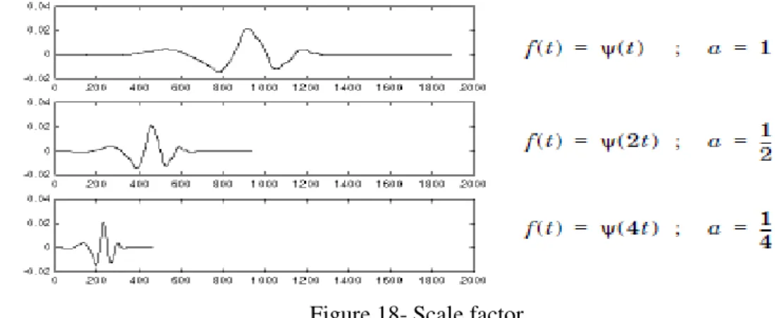
Scaling

Scaling a wavelet simply means stretching (or compressing) it











 −

=

a

b

t

a

t

b

a

ψ

ψ

(

)

1

77

Figure 17- Scaling a wavelet

The scale factor works exactly the same with wavelets. The smaller the scale factor, the more “compressed” the wavelet

Figure 18- Scale factor

Shifting

78

 Mathematically, delaying a function by k is represented by.

Figure 19- Wavelet function

Scale and Frequency: The more stretched the wavelet, the longer the portion of the signal with which it is being compared, and thus the coarser the signal features being measured by the wavelet coefficients.

79

There is a correspondence between wavelet scales and frequency as revealed by wavelet analysis:

Low scale a → Compressed wavelet → Rapidly changing details → High

frequency ω

High scale a → Stretched wavelet → Slowing changing, coarse features → Low

frequency ω

Types of Wavelet Transform:

 Continuous Wavelet Transform (CWT)

 Discrete Wavelet Transform (DWT)

Continuous Wavelet Transform: The continuous wavelet transform of a function is defined as;

(11)

where a is a scale parameter, b is translational parameter and ψ is wavelet

function.

Continuous Wavelet Transform: Similarly, the continuous wavelet transform is defined as the sum over all time of the signal multiplied by scaled, shifted versions of the wavelet function ψ:

(12)

The results of the continuous wavelet transform are many wavelet coefficients C, which are a function of scale and position.

Multiplying each coefficient by the appropriately scaled and shifted wavelet yields the constituent wavelets of the original signal.

dt

t

position

scale

t

f

position

scale

C

∫

=

(

)

(

,

,

)

)

,

(

ψ

dt

a

b

t

t

f

a

b

a

T

∫

∞ −



_







 −

=

1

(

)

ψ

80

Figure 21- Wavelet transform

Discrete Wavelet Transform: In continuous wavelet transform the dilation and translation parameters a and b vary continuously. Restricting a and

b to only discrete values of;

(13)

where the integers m and n control the wavelet dilation and translation

respectively.

is a specified fixed dilation step parameter set at a value greater than 1.

is the location parameter which must be greater than zero.

The control parameters m and n are contained in the set of all integers, both positive and negative.

Discrete Wavelet Transform: The wavelet transform of a continuous function (signal), using discrete wavelets can be written as;

(14)

m

a

a

=

m

a

nb

b

=

0

a

b

dt

nb

t

a

a

t

f

T

m

(

)

₂

(

)

81

are known as wavelet coefficients or detailed coefficients

Discrete Wavelet Transform;

 Separates the high and low-frequency portions of a signal through the use of filters

 One-Stage Filtering: Approximations and Details

 The approximations are the high-scale, low-frequency components of the signal

 The details are the low-scale, high-frequency components

Figure 22- Discrete wavelet transform; frequency portions of signal.

82

MULTIPLE-LEVEL DECOMPOSITION: One signal is broken down into many lower resolution components – wavelet decomposition tree

Figure 23- Multiple level decomposition. Wavelet Applications:

 Signal Processing

 Data Compression

83

 Biology for cell membrane recognition, to distinguish the normal from the pathological membranes

 DNA analysis, Protein analysis

 Blood-Pressure, Heart Rate and ECG analysis

 Finance for detecting the properties of quick variation of values

 In Internet traffic description, for designing the services size

 Industrial supervision of gear-wheel

 Speech Recognition

 Computer Graphics and Multifractal analysis

 Many areas of Physics- including molecular dynamics, astrophysics, optics, turbulence and quantum mechanics.

 Geophysical Study

3. ADAPTIVE NEURO FUZZY INFERENCE SYSTEM (ANFIS)

ANFIS Structure is given in the figure 20.

Figure 24- ANFIS Structure

A Two Rule Sugeno ANFIS has rules of the form:

(16)

(17)

Layer 1 Layer 2 Layer 3 Layer 4 Layer 5

w ₁ w ₁ w₁f₁

X

∏

N

∑ F

∏

N

Y w ₂ w ₂ w₂f₂

84

LAYER 1

is essentially the membership grade for x and y.

(18)

are parameters to be learnt. These are the premise parameters.

LAYER 2 (19) LAYER 3 (20) LAYER 4 (21)

are to be determined and are referred to as the consequent parameters. LAYER 5 (22)

4

,

3

)

(

2

,

1

)

(

=

=

=

=

−

x

for

i

O

i

for

x

O

µ

µ

i

b

c

a

,

,

)

(

x

O

a

c

x

x

1

1

)

(

−

+

=

µ

∑

∑

∑

=

=

i i i

i i i i

_w

f

w

f

w

O

2

,

1

),

(

)

(

2

=

w

=

x

y

i

=

O

i

i B

A i

i

µ

µ

2 1 , 3

w

w

w

w

O

i

=

=

₊

)

(

,

4i

w

f

w

p

x

q

y

r

O

=

=

+

+

85

4. APPLICATIONS

PREDICTION OF ALL INDIA SUMMER MONSOON RAINFALL (ISMR):

Study of All India Summer Monsoon Rainfall (ISMR);

 MONSOON MONTHS – JUNE, JULY, AUGUST & SEPTEMBER

 YEARS CONSIDERED – 1813 TO 2006 (194 YEARS)

 DISCRETE WAVELET TRANSFORM (DWT)

 ADAPTIVE NEURO FUZZY INFERENCE SYSTEM (ANFIS)

 MATLAB 2008

 www.tropmet.res.in

Figure 25- Adaptive Neuro Fuzzy Inference System (ANFIS) ANFI

Data Input

Wavelet

Decompositi Predicted

ANFI

Wavelet Reconstructio

86

0 20 40 60 80 100 120 140 160 180 200

600 650 700 750 800 850 900 950 1000 1050 1100

Years

Ra

in

fa

ll in

m

m

Actual Predicted

Figure 26- Comparison of Actual and Predicted Data Using ANFIS

0 20 40 60 80 100 120 140 160 180 200 800

820 840 860 880 900 920 940 960 980

Years

Ra

in

fa

ll in

m

m

Actual Predicted

87

0 20 40 60 80 100 120 140 160 180 200

-250 -200 -150 -100 -50 0 50 100 150 200

Years

Ra

in

fa

ll in

m

m

Actual Predicted

Figure 28- Comparison of Actual D1 and Predicted D1 Parameters

0 20 40 60 80 100 120 140 160 180 200

-150 -100 -50 0 50 100

Years

Ra

in

fa

ll in

m

m

Actual Predicted

88

0 20 40 60 80 100 120 140 160 180 200

-80 -60 -40 -20 0 20 40 60 80

Years

Ra

in

fa

ll in

m

m

Actual Predicted

Figure 30- Comparison of Actual D3 and Predicted D3 Parameters

0 20 40 60 80 100 120 140 160 180 200 600

650 700 750 800 850 900 950 1000 1050 1100

Years

R

ai

nf

al

l i

n m

m

Actual Predicted

89

Figure 32 -Comparison between Actual and Predicted Rainfall

PREDICTION OF ALL INDIA MINIMUM TEMPERATURE FOR JANUARY (AIMT):

Study of All India Minimum Temperature for January (AIMT)

 MINIMUM TEMPERATURE MONTH – JANUARY

 YEARS CONSIDERED – 1901 TO 2003 (103YEARS)

 DISCRETE WAVELET TRANSFORM (DWT)

 ADAPTIVE NEURO FUZZY INFERENCE SYSTEM (ANFIS)

 MATLAB 2008

90

0 10 20 30 40 50 60 70 80 90 100

85 90 95 100 105 110 115 120

Years

T

em

per

at

ur

e (

F

)

Actual Predicted

Figure 33- Comparison of Actual and Predicted Data Using ANFIS

0 10 20 30 40 50 60 70 80 90 100

96 98 100 102 104 106 108

Years

T

em

per

at

ur

e (

F

)

Actual Predicted

91

0 10 20 30 40 50 60 70 80 90 100

-10 -8 -6 -4 -2 0 2 4 6 8 10 Years T em per at ur e ( F ) Actual Predicted

Figure 35- Comparison of Actual D1 and Predicted D1 Parameters

0 10 20 30 40 50 60 70 80 90 100

85 90 95 100 105 110 115 120 Years T em per at ur e ( F ) Actual Predicted

92

0 10 20 30 40 50 60 70 80 90 100

-8 -6 -4 -2 0 2 4 6 8 10

Years

T

em

per

at

ur

e (

F

)

Actual Predicted

Figure 37-Comparison of Actual D3 and Predicted D3 Parameters

0 10 20 30 40 50 60 70 80 90 100

85 90 95 100 105 110 115 120

Years

T

em

per

at

ur

e (

F

)

Actual Predicted

93

94

5. CONCLUSION

 Wavelets offer a simultaneous localization in time and frequency domain.

 Using fast wavelet transform, it is computationally very fast.

 Able to separate the fine details in a signal. Very small wavelets can be used to isolate very fine details in a signal, while very large wavelets can identify coarse details.

 Wavelet transforms can be used to decompose a signal into component wavelets.

 In wavelet theory, it is often possible to obtain good approximation of the given function f by using only a few coefficients which is the great

achievement in compare to Fourier transform

 Wavelet theory is capable of revealing aspects of data that other signal analysis techniques miss the aspects like trends, breakdown points, and discontinuities in higher derivatives and self-similarity.

 It can often compress or de-noise a signal without appreciable degradation.

6.REFERENCES

Siddiqi, A. H., O. N. Uan, Z. Aslan, H.H. Öz, M. Zontul, G.Erdemir, (2009):