www.biogeosciences.net/14/597/2017/ doi:10.5194/bg-14-597-2017
© Author(s) 2017. CC Attribution 3.0 License.
Describing rainfall in northern Australia using
multiple climate indices
Cassandra Denise Wilks Rogers1and Jason Beringer1,2
1School of Earth, Atmosphere and Environment, Monash University, Clayton, 3800, Australia
2School of Earth and Environment (SEE), University of Western Australia, Crawley, WA, 6009, Australia
Correspondence to:Jason Beringer ([email protected]) Received: 2 May 2016 – Discussion started: 4 May 2016
Revised: 6 December 2016 – Accepted: 11 January 2017 – Published: 7 February 2017
Abstract. Savanna landscapes are globally extensive and highly sensitive to climate change, yet the physical processes and climate phenomena which affect them remain poorly un-derstood and therefore poorly represented in climate models. Both human populations and natural ecosystems are highly susceptible to precipitation variation in these regions due to the effects on water and food availability and atmosphere– biosphere energy fluxes. Here we quantify the relationship between climate phenomena and historical rainfall variability in Australian savannas and, in particular, how these relation-ships changed across a strong rainfall gradient, namely the North Australian Tropical Transect (NATT). Climate phe-nomena were described by 16 relevant climate indices and correlated against precipitation from 1900 to 2010 to deter-mine the relative importance of each climate index on sea-sonal, annual and decadal timescales. Precipitation trends, climate index trends and wet season characteristics have also been investigated using linear statistical methods. In general, climate index–rainfall correlations were stronger in the north of the NATT where annual rainfall variability was lower and a high proportion of rainfall fell during the wet season. This is consistent with a decreased influence of the Indian– Australian monsoon from the north to the south. Seasonal variation was most strongly correlated with the Australian Monsoon Index, whereas yearly variability was related to a greater number of climate indices, predominately the Tasman Sea and Indonesian sea surface temperature indices (both of which experienced a linear increase over the duration of the study) and the El Niño–Southern Oscillation indices. These findings highlight the importance of understanding the cli-matic processes driving variability and, subsequently, the im-portance of understanding the relationships between rainfall
and climatic phenomena in the Northern Territory in order to project future rainfall patterns in the region.
1 Introduction
and Tapper, 2006) among those known to have the greatest influence on Australian rainfall. Climatic phenomena, such as the Indian–Australian monsoon, affect rainfall and wa-ter balance on a seasonal scale (Sturman and Tapper, 2006). On longer timescales, natural climatic oscillations can cause interannual (e.g. ENSO) to decadal scale (e.g. the Pacific Decadal Oscillation) variability (Kamruzzaman et al., 2013). Ultimately rainfall is a complex part of the climate system that is dependent on many different factors, including various climatic phenomena, over many different timescales (Risbey et al., 2009).
One common method used to research the influence of cli-matic phenomena on various clicli-matic variables, such as rain-fall, is through the use of climate indices (e.g. Ashok et al., 2007; Kamruzzaman et al., 2013; Schepen et al., 2012). A climate index is a numerical value which provides a measure of the change away from the mean in an oscillatory climate system (National Center for Atmospheric Research, 2012). Climate indices generally consist of a single value, such as a measure of sea surface temperature (SST), mean sea level pressure (MSLP) or wind speed, which can be related via sta-tistical analysis to highly complex climatic processes. For ex-ample, Australian rainfall is well correlated with the South-ern Oscillation Index (SOI), which is in turn associated with ENSO (e.g. Murphy and Ribbe, 2004; Risbey et al., 2009; Schepen et al., 2012).
There remain many uncertainties surrounding the impacts that anthropogenic climate change will have on precipitation, which Rowell (2011) argues is because rainfall model unctainty in Australia is due to natural variation rather than er-rors in climate models or observational data. For example, in Queensland, Murphy and Ribbe (2004) found the rela-tionship between ENSO and rainfall did not remain constant over time. They ascribed this to the change in the status of the Interdecadal Pacific Oscillation. It is therefore important to better understand natural variation in circulatory climate systems to improve future climate projections. Over longer time periods, relationships between climatic phenomena may strengthen or weaken due to climate change. One potential major impact on Australian rainfall is an increase in north-ern Australian wet season rainfall due to an intensification of the monsoon. Kumar et al. (1999) observed an intensifi-cation of the monsoon due to a weakening in its relation-ship with ENSO. Climate change is also expected to alter other atmospheric circulation systems, such as the weaken-ing of the Walker circulation (Power and Smith, 2007; Vec-chi and Soden, 2007) and the broadening of the Hadley Cell (Brönnimann et al., 2009), making the potential impact of cli-mate change on precipitation in tropical Australia very uncer-tain. Understanding the relationship between climate drivers and rainfall under both natural variability and anthropogenic change is required to project the future impact of climate change on food, fibre and water production in savanna re-gions.
In Australia, rainfall variability is crucial to the structure and productivity of the landscape, particularly across the vast extent of the savanna biome which accounts for 25 % of the continent (Beringer et al., 2007, 2011b; Eamus et al., 2013; Haverd et al., 2016; Hutley et al., 2011; Kanniah et al., 2011). Not only do savanna landscapes cover a large portion of Australia, they also account for 15 % of the land surface of the planet (Beringer et al., 2011b). This area has the potential to increase in size due to climate change (Fran-chito et al., 2011), making the improved knowledge of these landscapes important in understanding future rainfall trends in Australia and around the world. Australian savannas re-main fairly undisturbed (Beringer et al., 2014), making them good for temporal change studies. Vegetation productivity, and hence the carbon balance, is vulnerable to changes in rainfall variability (Kanniah et al., 2011) because savanna structure, composition and function shift in response to short-term (monsoonal) and long-short-term (ENSO, Interdecadal Pa-cific Oscillation, PaPa-cific Decadal Oscillation Index (PDO), etc.) rainfall climatology (Beringer et al., 2011a). Moreover, disturbances, such as fire, cyclones and grazing, are also key drivers of savanna structure and productivity which are in turn driven by rainfall patterns (Beringer et al., 2007; Bond et al., 2003; Hutley and Beringer, 2011; Hutley et al., 2013). Savanna grass productivity is very sensitive to rain-fall and the biomass produced creates fodder for cattle and fuel for frequent burning, resulting in greenhouse gas emis-sions (Beringer et al., 1995, 2014; Moore et al., 2015, 2016). Therefore, evaluating the relationship between interannual variation in rainfall and climate phenomena is crucial for predicting the responses of the water, energy and carbon cy-cles of savanna vegetation (Beringer et al., 2011a; Kanniah et al., 2013). Despite this there has been a paucity of research undertaken on the climatic influences of rainfall in northern Australia and savannas; however, there have been a number of continental-scale analyses (e.g. Nicholls, 1989; Risbey et al., 2009; Schepen et al., 2012).
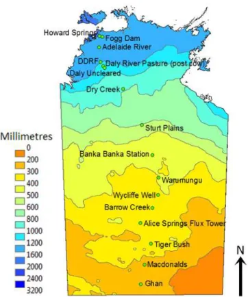
From north to south along the Northern Territory (NT), there is a substantial rainfall gradient (Table 1 and Fig. 1) known as the North Australian Tropical Transect (NATT). The north is highly seasonal with a characteristic tropical monsoonal climate (Bureau of Meteorology, 2011b; Hutley et al., 2011) and a rainy season between September and May (Nicholls et al., 1982; Suppiah and Hennessy, 1996), whereas the south is semi-arid to arid (Beringer et al., 2016) with very little seasonal variation in rainfall (Hennessy et al., 1999). A sharp change in rainfall rate occurs around Dry Creek, with the stations north of Dry Creek experiencing higher rainfall and the stations further south experiencing less rainfall.
Table 1.Names, locations and mean annual precipitation (MAP) for sites along the North Australian Tropical Transect. Values in brackets show coefficients of variation. MAP from AWAP data from 1900 to 2010.
Site name Abbreviated Latitude Longitude MAP
name (◦S) (◦E) (mm)
Howard Springs HS 12.49 131.15 1520 (19 %)
Fogg Dam FD 12.55 131.31 1423 (20 %)
Adelaide River AR 13.08 131.12 1318 (22 %)
DDRF DD 13.83 131.19 1100 (22 %)
Daly River Pasture (post cow) DR 14.06 131.32 1060 (21 %)
Daly Uncleared DU 14.16 131.39 1041 (22 %)
Dry Creek (a.k.a. Dry River) DC 15.26 132.37 762 (27 %)
Sturt Plains SP 17.15 133.35 521 (37 %)
Banka Banka Station BB 18.71 133.92 394 (45 %)
Warumungu Wa 19.89 134.25 345 (47 %)
Wycliffe Well WW 20.81 134.23 298 (50 %)
Barrow Creek BC 21.50 133.92 294 (55 %)
Alice Springs Flux Tower AS 22.28 133.25 288 (52 %)
Tiger Bush TB 23.37 133.84 274 (55 %)
MacDonalds Ma 24.47 133.47 225 (58 %)
Ghan Gh 25.50 133.25 189 (62 %)
31
Figure 1: Map of average annual rainfall (mm) from 1961 to 1990 (colours) and the location of each site along the North Australian Tropical Transect (Adapted from Bureau of Meteorology (2011a)).
5
Figure 1.Map of average annual rainfall (mm) from 1961 to 1990 (colours) and the location of each site along the North Australian Tropical Transect (adapted from Bureau of Meteorology, 2011a).
carbon and water balances illustrates the need to better un-derstand the climatic processes in these regions. This paper determines how well different climate indices describe
rain-fall along the NATT. This has been achieved using Pearson product-moment correlations. This research addresses cor-relation, not causation, over an extensive historical record (1900 to 2010). Trends in climate indices and rainfall over the NATT for this time period have also been examined. An un-precedented number of climate indices, representing climatic phenomena that are known to influence Australian rainfall variability, have been implemented in this research.
2 Methodology 2.1 Site description
This paper examines the strong rainfall gradient along an ex-tended version of the NATT, where 16 sites were chosen to examine the spatial relationships of rainfall with 16 different climate indices (Table 1 and Fig. 1). Due to the recognition of the importance of the NATT as a “living laboratory” (Hut-ley et al., 2011) and the role of rainfall is ecosystem structure and function (Beringer et al., 2011b), a number of microme-teorological flux measurements have been established along the NATT as part of the regional flux network (OzFlux). Beringer et al. (2016) provide a description of the OzFlux network with initial cross site analysis. Howard Springs has been a long-term monitoring site with observations initiated in 1996 (Eamus et al., 2001) and other sites include Fogg Dam (Beringer et al., 2013), Daly River (Hutley et al., 2011), Dry Creek (Beringer et al., 2011b) and Alice Springs (Clev-erly et al., 2013). Rainfall decreases along the NATT from approximately 1600 mm per year in the north, at a rate of
∼200 mm per degree, to approximately 200 mm per year in
Me-teorology, 2011a; Cook and Heerdegen, 2001) (Table 1 and Fig. 1). Associated with this decrease in precipitation is a change in vegetation structure and composition which varies from moist woodland savanna in the north to dry grasslands in the south (Beringer et al., 2011b; Hutley et al., 2011). Sea-sonality of rainfall also decreases from the north to the south, mostly due to the decrease in the influence of the monsoon moving further inland (Cook and Heerdegen, 2001). 2.2 Climate indices
We used an extensive 110 years of spatial data, from 1900 to 2010, to help identify persistent long-term correlations be-tween precipitation and climate indices and to capture mul-tiple events of each climatic phenomenon occurring at dif-ferent frequencies. We also advanced on previous studies by examining a vast number of climate indices (16) as described below and summarised in Table 2. The use of multiple mate indices enabled us to gain an insight into which cli-matic phenomena may have the strongest relationships with spatial rainfall patterns in the NT and, ultimately, which cli-matic phenomena may have an effect on ecosystem structure, function and distribution. A map showing the regions over which each climate index is calculated is shown in Fig. 2. 2.2.1 Indian Ocean and Indonesian phenomena Climatic phenomena over the Indian Ocean and Indone-sia are related to Australian precipitation both directly (e.g. Kamruzzaman et al., 2013) and indirectly by influencing other climatic phenomena (e.g. the Interdecadal Pacific Os-cillation and ENSO; Power et al., 1999). SST anomaly (SSTA) data over these regions were used to calculate four climate indices as follows (Table 2 and Fig. 2). The IOD, rep-resented by the Dipole Mode Index (DMI), is defined as the difference between the Indian Ocean West Pole Index (WPI: the average of the SSTAs over 50 to 70◦
E and 10◦
N to 10◦ S) and the Indian Ocean East Pole Index (EPI: the average of the SSTAs over 90 to 110◦
E and 0◦
N to 10◦
S; Saji et al., 1999). Changes in the DMI coincide with changes in equa-torial zonal wind variation (Saji et al., 1999). Anomalies in the DMI begin around June and increase until October when they reach a maximum, after which they quickly return to normal (Saji et al., 1999).
The Indonesia Index (II: the average of the SSTAs over 120 to 130◦E and 0◦N to 10◦S) characterises SSTAs over the Indonesian region and has been related to eastern Aus-tralian winter rainfall (Verdon and Franks, 2005) and NT rainfall (Schepen et al., 2012).
2.2.2 El Niño–Southern Oscillation
The relationship between ENSO and Australian rainfall is well known (e.g. Risbey et al., 2009; Ropelewski and Halpert, 1996). There are multiple ENSO indices of which we used six (Table 2 and Fig. 2). The SOI is commonly used
in Australian rainfall studies (e.g. Risbey et al., 2009; Ro-pelewski and Halpert, 1996; Schepen et al., 2012; Suppiah and Hennessy, 1996). The SOI for a given month is calcu-lated as a function of MSLP difference between Tahiti and Darwin (Bureau of Meteorology, 2012).
The four El Niño indices represent ENSO using SSTA measurements that are averaged over different regions of the Pacific Ocean (Fig. 2). These indices and their corresponding regions are the Extreme Eastern Tropical Pacific SST (Niño 1+2), 90 to 80◦W and 0◦N to 10◦S; the Eastern Tropical
Pacific SST (Niño 3), 150 to 90◦
W and 5◦
N to 5◦ S; the East Central Tropical Pacific SST (Niño 3.4), 170 to 120◦
W and 5◦
N to 5◦
S; and the Central Tropical Pacific SST (Niño 4), 160◦
E to 150◦
W and 5◦ N to 5◦
S (ESRL, 2012; Kam-ruzzaman et al., 2013; Risbey et al., 2009). KamKam-ruzzaman et al. (2013) noted a seasonal pattern in Niño 1+2 and Niño 3 from 1957 to 2007.
The El Niño Modoki Index (EMI) quantifies ENSO Modoki events, which are similar to traditional ENSO events (Ashok et al., 2007), but with the maximum warming further east than normal (Risbey et al., 2009). The EMI is defined by the following equation:
EMI=C−0.5·(E+W ), (1)
whereCrepresents SSTAs over 165◦
E to 140◦
W and 10◦ N to 10◦
S,Erepresents SSTAs over 110 to 70◦
W and 5◦ N to 15◦
S andW represents SSTAs over 125 to 145◦
E and 20◦ N to 10◦S (Ashok et al., 2007; Schepen et al., 2012).
2.2.3 Extratropical phenomena
The Tasman Sea Index (TSI), defined as an area off the east coast of Australia bounded by 150 to 160◦
E and 30 to 40◦ S (Murphy and Timbal, 2008), was included in this research to investigate whether there is a potential link between extrat-ropical SSTs and NT rainfall (Table 2 and Fig. 2). We used the average of the SSTAs over this area to calculate the TSI. The use of the TSI to quantify extratropical SSTs has only been used in recent years (e.g. Murphy and Timbal, 2008; Schepen et al., 2012) so there are not many studies that in-clude this index.
2.2.4 Atlantic and tropical phenomena
Links have been found between Atlantic Ocean SSTs and rainfall in south-eastern (Kamruzzaman et al., 2013) and north-western Australia (Lin and Li, 2012). The North At-lantic Index (NATL: average SSTA over 60 to 30◦
W and 20 to 5◦
N) and the South Atlantic Index (SATL: average SSTA over 30◦
W to 10◦
E and 0◦
N to 20◦
32
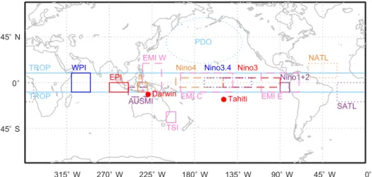
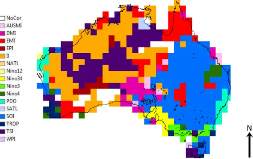
Figure 2: Approximate climate index measurement regions. Climate indices are calculated over the following areas: WPI – solid blue rectangle, EPI – solid red rectangle, DMI – the difference between the WPI and the EPI, SOI – calculated using MSLP measurements at Tahiti and Darwin (red dots), TSI – solid pink rectangle, Niño 1+2 – solid purple rectangle, Niño 3 – dashed red rectangle, Niño 3.4 – dotted blue rectangle, Niño 4 – dashed orange rectangle, NATL – dotted orange rectangle, SATL – dotted 5
purple rectangle, TROP – calculated between top and bottom light blue lines, EMI – calculated using areas enclosed by dashed pink rectangles, II – solid orange rectangle, AUSMI – dashed purple rectangle and PDO – dashed light blue oval (note: PDO is calculated over the entire area of the Pacific Ocean north of 20°N, the oval is only included for illustrative purposes). Figure produced using definitions for climate indices listed in Section 2.2.
10
315° W 270° W 225° W 180° W 135° W 90° W 45° W 0° 45° S
0° 45° N
TROP
TROP
NATL
SATL AUSMI
WPI
EPI II Nino4 Nino3.4 Nino3 Nino1+2
EMI C EMI E
EMI W
TSI
Tahiti Darwin
PDO
Figure 2. Approximate climate index measurement regions. Climate indices are calculated over the following areas: WPI – solid blue rectangle, EPI – solid red rectangle, DMI – the difference between the WPI and the EPI, SOI – calculated using MSLP measurements at Tahiti and Darwin (red dots), TSI – solid pink rectangle, Niño 1+2 – solid purple rectangle, Niño 3 – dashed red rectangle, Niño 3.4 – dotted blue rectangle, Niño 4 – dashed orange rectangle, NATL – dotted orange rectangle, SATL – dotted purple rectangle, TROP – calculated between top and bottom light blue lines, EMI – calculated using areas enclosed by dashed pink rectangles, II – solid orange rectangle, AUSMI – dashed purple rectangle, and PDO – dashed light blue oval (note: PDO is calculated over the entire area of the Pacific Ocean north of 20◦N; the oval is only included for illustrative purposes). Figure produced using definitions for climate indices listed in Sect. 2.2.
presence of a seasonal pattern in the NATL and the SATL as well as an increasing trend in both from 1957 to 2007.
SSTs from the tropical regions in the Pacific, Atlantic and Indian oceans all have links with Australian rainfall (Lin and Li, 2012; Risbey et al., 2009; Schepen et al., 2012). The Global Tropics Index (TROP: the average of the SSTAs between 10◦N and 10◦S around the equator; Na-tional Oceanic and Atmospheric Administration, 2012) in-corporates all three of the above mentioned oceans into one climate index (Table 2 and Fig. 2). Correlations have been found between south-eastern Australian rainfall and TROP (Kamruzzaman et al., 2013). Kamruzzaman et al. (2013) noted the presence of a seasonal pattern in TROP as well as a quadratic trend from 1957 to 2007.
2.2.5 Indian–Australian monsoon
The Indian–Australian monsoon is highly influential on trop-ical Australian rainfall (Sturman and Tapper, 2006) and is characterised by the reversal of easterly trade winds in the Australian tropics (Hendon et al., 2012). Kajikawa et al. (2009) reason that Indian–Australian monsoon variabil-ity can be depicted using a measurement of average zonal wind (U-wind) velocity at 850 mb over 110 to 130◦
E and 5 to 15◦
S, known as the Australian Monsoon Index (AUSMI, Table 2 and Fig. 2), but the definition used for this research differed slightly (see Sect. 2.3.3). AUSMI is negative for the majority of the year, when the easterly trade winds are dominant, until the start of the monsoon when these winds weaken and then become positive. Kajikawa et al. (2009) found AUSMI to be a good predictor of variability in the
monsoon on seasonal, intraseasonal, interannual and inter-decadal timescales.
2.2.6 The Pacific Decadal Oscillation
The PDO is a measure of the Pacific Decadal Oscillation, a shift in Pacific Ocean temperatures that has a period of 20 to 30 years (Joint Institute for the Study of the Atmosphere and Ocean, 2012). The Pacific Decadal Oscillation is known to affect rainfall and global temperatures (Franks, 2002; Kam-ruzzaman et al., 2013). The PDO is defined as the leading principal component of SSTs in the north Pacific (Joint Insti-tute for the Study of the Atmosphere and Ocean 2012) (Ta-ble 2 and Fig. 2). The causes of the Pacific Decadal Oscilla-tion remain unknown; therefore it is not possible to predict changes in the PDO (Joint Institute for the Study of the At-mosphere and Ocean, 2012). This limits the usefulness of the PDO for forecasting climate variability. Note, the Inter-decadal Pacific Oscillation was not included in this research as it is highly correlated with the Pacific Decadal Oscillation (Franks, 2002).
2.3 Data description and sources
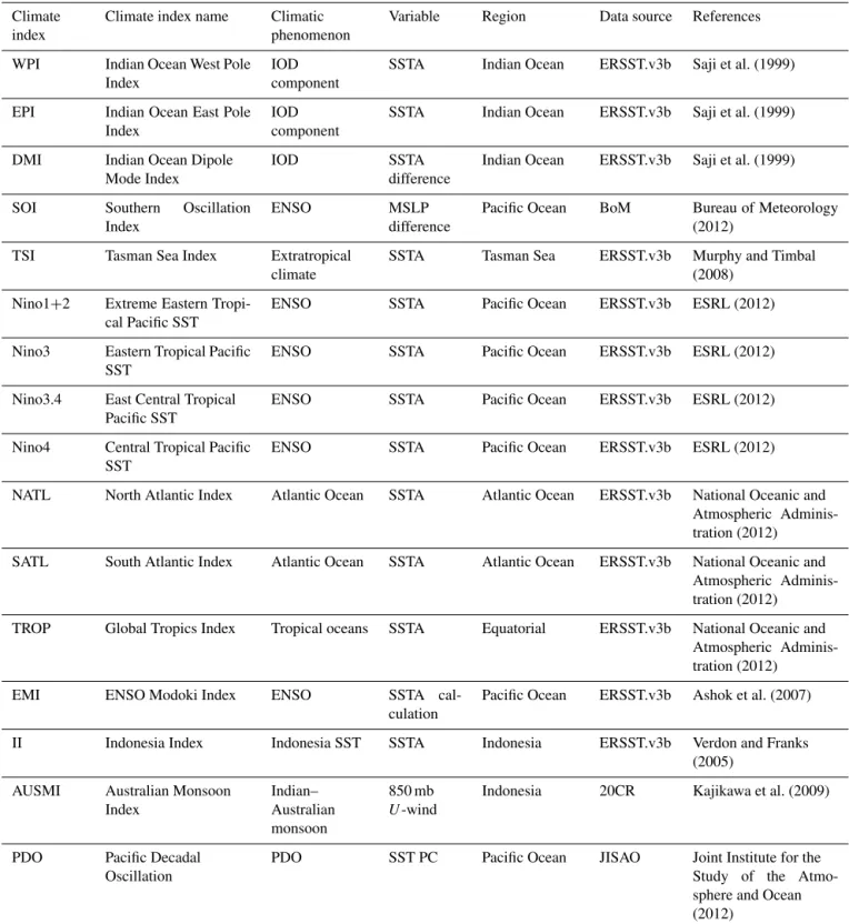
Table 2.Climate index information showing index name, related climatic phenomenon, variable measured, region of influence, data source and a key reference.
Climate index
Climate index name Climatic phenomenon
Variable Region Data source References
WPI Indian Ocean West Pole Index
IOD component
SSTA Indian Ocean ERSST.v3b Saji et al. (1999)
EPI Indian Ocean East Pole Index
IOD component
SSTA Indian Ocean ERSST.v3b Saji et al. (1999)
DMI Indian Ocean Dipole Mode Index
IOD SSTA
difference
Indian Ocean ERSST.v3b Saji et al. (1999)
SOI Southern Oscillation Index
ENSO MSLP
difference
Pacific Ocean BoM Bureau of Meteorology (2012)
TSI Tasman Sea Index Extratropical climate
SSTA Tasman Sea ERSST.v3b Murphy and Timbal (2008)
Nino1+2 Extreme Eastern Tropi-cal Pacific SST
ENSO SSTA Pacific Ocean ERSST.v3b ESRL (2012)
Nino3 Eastern Tropical Pacific SST
ENSO SSTA Pacific Ocean ERSST.v3b ESRL (2012)
Nino3.4 East Central Tropical Pacific SST
ENSO SSTA Pacific Ocean ERSST.v3b ESRL (2012)
Nino4 Central Tropical Pacific SST
ENSO SSTA Pacific Ocean ERSST.v3b ESRL (2012)
NATL North Atlantic Index Atlantic Ocean SSTA Atlantic Ocean ERSST.v3b National Oceanic and Atmospheric Adminis-tration (2012)
SATL South Atlantic Index Atlantic Ocean SSTA Atlantic Ocean ERSST.v3b National Oceanic and Atmospheric Adminis-tration (2012)
TROP Global Tropics Index Tropical oceans SSTA Equatorial ERSST.v3b National Oceanic and Atmospheric Adminis-tration (2012)
EMI ENSO Modoki Index ENSO SSTA
cal-culation
Pacific Ocean ERSST.v3b Ashok et al. (2007)
II Indonesia Index Indonesia SST SSTA Indonesia ERSST.v3b Verdon and Franks
(2005)
AUSMI Australian Monsoon Index
Indian– Australian monsoon
850 mb U-wind
Indonesia 20CR Kajikawa et al. (2009)
PDO Pacific Decadal Oscillation
PDO SST PC Pacific Ocean JISAO Joint Institute for the Study of the Atmo-sphere and Ocean (2012)
June to 31 August, and 1 September to 30 November, respec-tively). Unless otherwise stated, rainfall data will be reported as daily averages to remove any inconsistencies created by differing season or month lengths. We defined a year to start on 1 July and end on 30 June (the hydrological year) so that
2.3.1 Precipitation data
Australian gridded daily rainfall data, interpolated from sta-tion data (1900 to 2010), were obtained from the Australian Water Availability Project (AWAP) (Raupach et al., 2009, 2012), which was developed by the Commonwealth Scien-tific and Industrial Research Organisation (CSIRO). AWAP resolution is 0.05◦
latitude by 0.05◦
longitude, approximately 5 km by 5 km (CSIRO, 2012). While AWAP data were avail-able nationally from 1900 to 2010, at specific sites there were a very small number of missing values (∼0.1 % at
the NATT sites). At the NATT sites, in the case of a single missing point, data were linearly interpolated. For consecu-tive missing values, daily averages for each month (excluding months with missing data) were calculated for each location and these averages replaced the missing values for the corre-sponding month.
2.3.2 Sea surface temperature indices and ENSO data PDO data were obtained from the Joint Institute for the Study of the Atmosphere and Ocean (JISAO), Washing-ton University (http://jisao.washingWashing-ton.edu/pdo/PDO.latest). SSTA data for the WPI, EPI, DMI, TSI, Niño1+2, Niño3,
Niño3.4, Niño4, NATL, SATL, TROP, EMI and II were ex-tracted from the Extended Reconstruction Sea Surface Tem-perature version 3b (ERSST.v3b) via the National Oceanic and Atmospheric Administration (NOAA) – National Oper-ational Model Archive and Distribution System (NOMADS) Live Access Server (LAS) (http://nomads.ncdc.noaa.gov/las/ getUI.do). ERSST.v3b is based on the International Compre-hensive Ocean-Atmosphere Data Set (ICOADS) release 2.4 (National Climatic Data Center, 2012). For more information about past ERSST versions see T. M. Smith et al. (2008). ERSST.v3b produces monthly SST and SSTA data over 2◦ grid boxes (Xue et al., 2010) using buoy and ship observa-tions (National Climatic Data Center, 2012; T. M. Smith et al., 2008; Yates et al., 2008). Data obtained from ERSST.v3b may be prone to uncertainty created by incomplete sam-pling or data errors (T. M. Smith et al., 2008). Anomaly data are then created using a base period climatology from 1971 to 2000 following Xue et al. (2010). Monthly SSTA data were available from the 1854 to 2012 reconstruction, but data before 1940 are considered less reliable (NCDC, 2012). The use of SSTAs for some of these indices is con-sistent with other climate index research, e.g. WPI, EPI, DMI, Niño3, Niño3.4, Niño4, EMI, II and TSI by Schepen et al. (2012) and the Niño indices, SOI, PDO, DMI, NATL, SATL and TROP by Kamruzzaman et al. (2013). SOI data were obtained from the Australian Bureau of Meteorology (http://www.bom.gov.au/climate/current/soihtm1.shtml).
2.3.3 Monsoon index data
The definition used for AUSMI in this research is slightly different to that used by Kajikawa et al. (2009) and was instead defined as the 850 mb zonal wind velocity av-eraged over the area enclosed within 110 to 130◦
E and 6 to 14◦
S. Eastward zonal wind velocity (m s−1) data
were extracted from the NOAA Cooperative Institute for Research in Environmental Sciences (CIRES) 20th Cen-tury Reanalysis version 2 (20CR): monthly mean pres-sure level data at 850 mb. The 20CR provides reanalysed weather data over time and space from the late 1800s to the present (http://www.esrl.noaa.gov/psd/data/gridded/data. 20thC_ReanV2.pressure.mm.html). The 20CR data were made available by the NOAA/Office of Ocean and Atmo-spheric Research (OAR)/Earth Systems Research Labora-tory, Physical Sciences Division (ESRL, 2012), Boulder, Colorado, USA. The data were extracted for the latitudes 6, 8, 10, 12 and 14◦
S and for the longitudes 110, 112, 114, 116, 118, 120, 122, 124, 126, 128 and 130◦
E. Since the data were only available for every 2◦
of latitude it was not possible to be exactly consistent with Kajikawa et al. (2009). Once the data were extracted they were averaged over the specified region to produce a one dimensional time series.
2.4 Trends
Before we assessed correlations between precipitation and climate indices we examined for linear trends in both the rainfall data and the climate indices. Linear regression and smoothing were used to identify persistent linear trends be-tween 1900 and 2010.
2.5 Correlation maps
Maps of the correlations between rainfall and climate indices were created using Pearson product-moment correlation co-efficients of determination (r2values) to quantify the correla-tions between rainfall and climate indices for every grid point (5 km resolution) across Australia using the gridded meteo-rological AWAP data. Significance was assessed through p values at the 95 % significance level and only significant data were plotted throughout this research. Maps ofr2andp val-ues were used to determine which climate index was cor-related best with rainfall at each grid point over Australia. These maps were spatially aggregated from 0.05◦
×0.05◦ to 1.25◦
×1.25◦
2.6 Point correlations
Correlation strengths between rainfall and each climate in-dex were determined for every site along the NATT (Table 1 and Fig. 1) for monthly, seasonal and annual time periods. These correlations are referred to throughout the paper as point correlations. The point correlations allowed for an in depth analysis of which climate indices were most highly correlated with rainfall along the rainfall gradient (i.e. NATT) by providing a visual comparison of the relative correlation strengths of multiple indices in two dimensions.
For the purposes of this research,r2greater than 0.6 was considered very strong, between 0.2 and 0.6 was considered strong, between 0.1 and 0.2 was considered moderate and less than 0.1 was considered weak. These definitions were based on analysis done by Murphy and Ribbe (2004), Sup-piah (2004) and SupSup-piah and Hennessy (1996) and were mainly intended to be used to compare relative correlation strengths between different indices, rather than to determine a definitive measure of strength. To compare point correla-tion strengths between climate indices over each time period, a numerical rank, referred to in this research as an index rank, was calculated. Each climate index was given a rank from 1 (strongest correlation) to 16 (weakest correlation) for each site along the NATT. The average rank over all sites for each climate index was then used to find which indices showed, on average, the strongest correlations along the entire NATT.
2.7 Wet season characteristics
Wet season start (onset) date was defined as the date when rainfall, between 1 September and 30 April the following year, exceeded 15 % of the rainfall total between these two dates (I. N. Smith et al., 2008). This definition was created by I. N. Smith et al. (2008) who cited a similar definition by Nicholls (1984). Wet season end (retreat) date was defined as the date when rainfall, between 1 September and 30 April, exceeded 85 % of the total rainfall (I. N. Smith et al., 2008). The time between the start and end date is referred to as the wet season. Wet season onset and retreat is not to be con-fused with the monsoon onset and retreat. During the wet season the tropics experience heavy precipitation. Similarly, the monsoon is characterised by heavy rainfall but, unlike the wet season, the monsoon is also characterised by shifts in the wind and pressure in the region. Any single wet season typ-ically consists of multiple monsoon active and break phases (Suppiah and Hennessy, 1996) but these have not been exam-ined in this research. The wet season definition used for this research was chosen as it should cover all monsoon active phases and ensure that both start and end dates exist for each site along the NATT for every year. Values were calculated for mean total wet season rainfall, maximum and minimum total, average wet season start and end date, average duration, number of rain days (number of days during the wet season
where rainfall is greater than zero) and rainfall intensity for each NATT site.
2.8 Limitations
One limitation of this study was the lack of inclusion of in-dices which measure the Madden–Julian Oscillation and the Southern Annular Mode. An area of further research for this study could include the inclusion of these phenomena but this may require significantly shortening the study period. Data accuracy in observational, reconstructed and modelled data has implications on the correlations determined in this re-search. The length of this study poses some issues due to changes in observational equipment used to measure envi-ronmental variables and reduced spatial coverage of record-ing stations or gauges in the past. For example, ERSST.v3b data quality is compromised by a cold bias evident in histori-cal SST data around the 1940s. This bias is due to changes in observational methods associated with World War II (Smith and Reynolds, 2003). Additionally, AWAP data accuracy is limited by the sparseness of observation points (CSIRO, 2012).
3 Results and discussion 3.1 Trend analysis
Linear trends in rainfall and each climate index were anal-ysed over the full 110-year time period. Fractional rainfall change was calculated for each site over the NATT, revealing a significant increase in rainfall at all sites (Table 3). Hen-nessy et al. (1999), Li et al. (2012) and Nicholls (2006) all noted similar rainfall trends from 1910 to 1995, 1948 to 2007 and 1950 to 2005, respectively, but only Li et al. (2012) found the increase was significant. While the increase in rainfall in the north was mostly greater in magnitude than in the south, rainfall change in the south was more variable and less linear (Table 3). The dominant influence of the monsoon on north-ern rainfall (Sturman and Tapper, 2006) is likely to explain these observations of generally high summer and low win-ter rainfall in the north, whereas the low rainfall in the south has many different and inconsistent influences (Beringer and Tapper, 2000; Sturman and Tapper, 2006; Suppiah and Hen-nessy, 1996).
Table 3.Temporal rainfall trends using linear regression of annual data along the NATT for the period 1900 to 2010. Italicised and boldr2 values are significant at the 95 % significance level (i.e. all trends are significant). Strength shows the goodness of fit of the linear trend line. Absolute gradient shows the actual increase in annual rainfall per decade. Fractional gradient shows the increase in annual rainfall per decade of a site relative to the mean rainfall at that site. Brackets indicate the sign of the linear trend if significant. Coefficient of variation shows the variability of each site as a percentage of the sites annual average rainfall.
Site Latitude Correlation Absolute gradient Fractional gradient coefficient (◦S) Coefficient (r2) (mm decade−1) (% change per decade) of variation
HS 12.49 0.14 33.20 (+) 2.18 (+) 19 %
FD 12.55 0.17 36.52 (+) 2.57 (+) 20 %
AR 13.08 0.22 41.71 (+) 3.16 (+) 22 %
DD 13.83 0.16 29.82 (+) 2.71 (+) 22 %
DR 14.06 0.17 28.52 (+) 2.69 (+) 21 %
DU 14.16 0.19 30.25 (+) 2.91 (+) 22 %
DC 15.26 0.22 30.54 (+) 4.01 (+) 27 %
SP 17.15 0.13 21.77 (+) 4.18 (+) 37 %
BB 18.71 0.04 10.78 (+) 2.74 (+) 45 %
Wa 19.89 0.06 12.60 (+) 3.65 (+) 47 %
WW 20.81 0.11 14.99 (+) 5.02 (+) 50 %
BC 21.50 0.10 15.76 (+) 5.35 (+) 55 %
AS 22.28 0.10 14.55 (+) 5.06 (+) 52 %
TB 23.37 0.06 11.10 (+) 4.05 (+) 55 %
Ma 24.47 0.06 9.70 (+) 4.32 (+) 58 %
Gh 25.50 0.06 8.64 (+) 4.57 (+) 62 %
been documented; for example Vecchi and Soden (2007) noted a weakening in the Walker circulation while Power and Smith (2007) noted a reduction in the magnitude of the SOI and the possible dominance of an El Niño pattern from 1977 to 2006. Kumar et al. (1999) noted a weakening in the re-lationship between ENSO and the monsoon, leading to an intensification of the monsoon, and Nicholls et al. (1996) ob-served a reduction in the SOI due to a change in the relation-ship between Australian rainfall, temperature and the SOI.
AUSMI showed a fairly weak but significant negative lin-ear trend over the study period. This finding suggests a weakening of the monsoon or a reduction in the duration of time when the monsoon is active. The observed decrease in AUSMI appears to contradict the observed precipitation in-crease over the NATT (Table 3), but the reduction in AUSMI is evidence not that the monsoon has weakened but rather that its circulation characteristics may have changed. Rain-fall was also observed to have increased in northern Western Australia, which has been linked to an increase in aerosol emissions originating from Asian population centres (Rot-stayn et al., 2007). This may help to explain the trends along the NATT but, as noted by Rotstayn et al. (2007), more re-search is required before a link between Asian aerosols and Australian rainfall can be determined.
It is important to note that since we have not detrended rainfall or climate index data, relationships between rainfall and any of WPI, EPI, TSI, Niño1+2, Niño3, Niño3.4, Niño4,
NATL, SATL, TROP, II and AUSMI (all of which show a linear trend) may be due to coincident trends rather than
any physical relationship between the given climatic phe-nomenon and rainfall. Any relationships between rainfall and the climate indices that did not show any linear trends (DMI, SOI, EMI and PDO) are less likely to be coincidental. 3.2 Seasonality
Northern Australia and the north of the NATT have a highly seasonal climate. The wet season, as defined in the meth-ods section, accounted for between 60 and 74 % of annual rainfall along the NATT from 1900 and 2010. The fact that most precipitation occurred during this period demonstrates the importance of understanding wet season dynamics. Both the number of rain days and the intensity of rainfall on these days showed a decreasing non-linear trend from the north to the south of the NATT.
Figure 3.Wet season characteristics for each site along the NATT (Table 1) for the period 1900 to 2010. Sites are plotted as their lat-itude along the transect. Average wet season start day, end day and duration are given. Start and end days are defined as the date when rainfall, between September 1 and April 30 the following year, ex-ceeded 15 and 85 %, respectively, of the total rainfall between these two dates (I. N. Smith et al., 2008a). Start and end days are dis-played as the number of days from 1 September. Wet season dura-tion is shown by the grey line connecting start and end days.
occurred earlier in the south (Fig. 3). The duration of the wet season was shortest in the northern half of the NATT and in-creased southward. Beyond about 19◦south, rainfall became more variable and less seasonal, producing earlier and longer calculated wet seasons (Fig. 3). The annual mean wet season rainfall volume decreased from the north to the south of the NATT (Fig. 4). Rainfall in the north was normally distributed whereas in the south it showed a positive skew. Standard de-viations were greatest in the north whereas coefficients of variability were greatest in the south, showing that precipita-tion variability was greatest in the south with respect to mean annual rainfall.
From the above discussion it is clear that relative variabil-ity in wet season total, start and end date, duration, number of rain days and intensity were all greater in the south of the NATT. These findings are consistent with the earlier re-sults that annual relative rainfall variability was greatest in the south. The lower variability in the north was most likely due to the dominance of the monsoon, creating relatively consistently high rainfall every year, whereas, as discussed earlier, rainfall in the south was affected by more factors, the strength of which vary from year to year such as incursion of cold fronts (Beringer and Tapper, 2000).
3.3 Rainfall–climate index correlations
Correlations between rainfall and climate indices were de-termined along the NATT (Figs. 7 and 8) and over Australia using gridded AWAP rainfall data at a 5 km resolution. Maps are displayed at a 125 km resolution for clarity of viewing
Figure 4.Mean annual wet season rainfall (mm) from 1900 to 2010 for each site along the NATT (Table 1). Boxes show 1 standard devi-ation and whiskers show maximum and minimum seasonal rainfall for each site.
(Figs. 5 and 6). The highest statistically significant correla-tions, on both seasonal and yearly timescales, were found be-tween rainfall and SOI, AUSMI, II, TSI, EMI and, to a lesser degree, EPI (Tables 4 and 5; Figs. 5, 6, 7 and 8). The rel-atively high correlations between these indices and rainfall indicates there may exist teleconnections between NT rain-fall and Indonesian, Tasman and Pacific SSTs and the climate phenomena that affect these regions, mainly the monsoon, ENSO and the IOD, but further research would be required to determine any mechanistic links, particularly as these re-lationships may be coincidental due to the linear trends in rainfall, AUSMI, II, TSI and EPI. While most climate in-dices chosen for this study showed some significant correla-tions with rainfall, some did not; these were SATL (except for correlations with annual data), NATL, TROP and PDO. This finding suggests that NT rainfall may not show a concurrent, linear relationship with Atlantic and tropical SSTs, north Pa-cific decadal SST variability and the climate phenomena that affect these regions.
3.3.1 Correlations between monthly rainfall and climate index data
ab-Table 4.Table shows the first three most highly correlated indices with rainfall at each site over the NATT (Table 1) for the period 1900 to 2010. Correlations are shown using the monthly data and interannual correlations are provided using the annual data. In addition, annual correlations are computed for the individual seasons only. Only correlations significant at the 95 % level are shown. Superscripts represent in which region the climate index is located and are defined as follows: IND is Indonesia and Indian Ocean, PAC is Pacific Ocean, TAS is Tasman Sea, and ATL is Atlantic and Tropical ocean. The first column for each time period in this table (i.e. the “1” columns) are shown in Fig. 5.
Site (°S) Lat
Monthly Annual Summer Autumn Winter Spring
1 2 3 1 2 3 1 2 3 1 2 3 1 2 3 1 2 3
HS 12.5 AUSMI SOI WPI SOI TSI II AUSMI SOI TSI AUSMI EMI SOI SOI - - SOI Nino3.4 Nino3
FD 12.6 AUSMI SOI WPI TSI II SOI AUSMI SOI TSI AUSMI SATL SOI SOI - - SOI II Nino3.4
AR 13.1 AUSMI SOI WP
I TSI II SOI AUSMI TSI SOI AUSMI EMI SATL SOI II - II SOI EPI
DD 13.8 AUSMI SOI DMI TSI EMI II AUSMI TSI SOI AUSMI EMI SOI SOI II AUSMI II EPI SOI
DR 14.1 AUSMI SOI DMI TSI II EMI AUSMI SOI TSI AUSMI EMI SOI SOI - - II EPI SOI
DU 14.2 AUSMI SOI WP
I TSI II EMI AUSMI TSI SOI AUSMI EMI SOI - - - II SOI EPI
DC 15.3 AUSMI SOI WPI II TSI SATL AUSMI SOI TSI AUSMI SATL SOI SOI II - SOI II DMI
SP 17.2 AUSMI SOI WP
I TSI SOI II AUSMI SOI TSI AUSMI SOI - SOI II Nino3.4 SOI II TSI
BB 18.7 AUSMI SOI DMI TSI AUSMI SOI AUSMI SOI TSI AUSMI - - SOI AUSMI II SOI DMI Nino3.4
Wa 19.9 AUSMI SOI WPI AUSMI TSI - AUSMI SOI TSI AUSMI - - SOI AUSMI SATL SOI II EPI
WW 20.8 AUSMI SOI TSI TSI II AUSMI AUSMI SOI DMI TSI AUSMI - SOI II AUSMI II SOI TSI
BC 21.5 AUSMI SOI TSI TSI II AUSMI AUSMI TSI DMI AUSMI - - AUSMI SOI WPI II SOI AUSMI
AS 22.3 AUSMI SOI TSI TSI II AUSMI TSI AUSMI SATL AUSMI TSI - AUSMI WPI SOI II EPI SOI
TB 23.4 AUSMI SOI TSI TSI AUSMI SOI AUSMI SOI TSI AUSMI TSI - AUSMI II SOI SOI II TSI
Ma 24.5 AUSMI SOI TSI TSI AUSMI SATL AUSMI SOI - AUSMI TSI - AUSMI II SOI SOI II AUSMI
Gh 25.5 AUSMI SOI II TSI II EMI AUSMI - - TSI AUSMI II II DMI AUSMI II SOI EPI
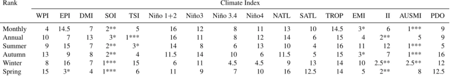
Table 5.Ranks showing relative correlation strengths of each climate index with precipitation over monthly, annual and seasonal time periods. Each rank shows, on average, which climate index has the highest correlation with rainfall at all sites along the NATT from July 1900 to June 2010 (except winter which uses calendar year from 1900 to 2009, not hydrological year). For example, on a monthly timescale AUSMI, on average, is the most highly correlated climate index over the entire NATT, SOI is the second most highly correlated, EMI is the third highest, and so on. Note, this table does not take statistical significance into account. First ***, second ** and third * highest correlations are given a number of asterisks for clarity.
Rank Climate Index
WPI EPI DMI SOI TSI Niño 1+2 Niño3 Niño 3.4 Niño4 NATL SATL TROP EMI II AUSMI PDO
Monthly 4 14.5 7 2** 5 16 12 8 11 13 10 14.5 3* 6 1*** 9
Annual 10 7 13 3* 1*** 16 11 8 12 14 6 15 4 2** 5 9
Summer 9 15 7 2** 3* 14 8 6 13 10 4 16 11 12 1*** 5
Autumn 13 9 8 2** 4 11.5 14 10 6 11.5 5 15 3* 7 1*** 16
Winter 8 16 7 1*** 15 6 11 4.5 4.5 9 13 14 10 2.5** 2.5** 12
Spring 15 3* 4 1*** 6 11 9 7 10 16 12.5 14 5 2** 8 12.5
solute rainfall trends were greatest in the north, but relative rainfall trends were greatest in the south. Correlations be-tween rainfall and both SOI and EMI were consistently weak along the entire NATT (Fig. 8a). AUSMI was the most highly correlated climate index spatially over the greater northern Australian region (Fig. 5). AUSMI was also correlated over a large portion of southern Australia, including almost all of Tasmania (the southern-most region of Australia, Fig. 5), suggesting this relationship is an artefact since the monsoon is known to not extend this far south (Bureau of Meteorol-ogy, 2008). The seasonal wind shift associated with AUSMI is linked to the wet summer and dry winter seasons in tropical
there-fore use caution when interpreting the results of this analysis. The AUSMI–rainfall correlation gradient was negative, very strong and highly linear (r2=0.9850) (Fig. 8a), reflecting the strong gradient in rainfall seasonality from the north to the south.
3.3.2 Correlations between yearly rainfall and climate index data
To examine annual to decadal correlations, annual rainfall data were examined. The three climate indices with the strongest correlations with annual rainfall over the NATT were TSI, II and SOI, all of which had similar correlation strengths (Figs. 6 and 8b). In general, correlations were mod-erate to strong in the north and weak to modmod-erate in the south, showing that rainfall variability became less well de-scribed by these climate indices southwards along the NATT (Fig. 8b).
The fact that TSI and rainfall were more strongly corre-lated in the north than the south of the NATT (Fig. 8b) was surprising since the TSI region of measurement is geograph-ically closer to the southern end of the transect (see Fig. 2). Frontal weather systems are likely to directly affect both the TSI region of measurement and the southern NATT but not the northern NATT, further suggesting that we would expect TSI to be more strongly related to southern NATT rainfall. Our results are not consistent with Schepen et al. (2012) who found TSI–rainfall correlations, using a 1-month lag, to be greatest in the south-west or the centre of the NT between 1950 and 2009 between October and January. Our research suggests that the correlations persisted for the entire year as we found significant correlations using annually averaged data (Fig. 8b). Sturman and Tapper (2006) noted a strong re-lationship between monsoon onset and synoptic weather in the extratropics. This relationship may help to explain the high correlations between TSI and NATT precipitation. Al-though, as mentioned earlier, both the TSI and rainfall have a significant linear trend which may produce higher correla-tions than are realistic.
One hypothesis to explain the correlations between Tas-man Sea SSTs and NT rainfall is the link both have with Rossby waves (planetary-scale atmospheric waves that cir-cle the South Pole) and extratropical weather events. Rossby waves are known to have a strong relationship with extrat-ropical weather events including high and low pressure cells (Kump et al., 2010; Sturman and Tapper, 2006) and display coupling with global SSTs (Hill et al., 2000). Therefore, the TSI–NATT rainfall correlations could be due to the simulta-neous effects of Rossby waves on both extratropical weather, which are known to affect NT rainfall (Sturman and Tapper, 2006) and Tasman Sea SSTs. Additional research is neces-sary to further investigate this hypothesis.
3.3.3 Annual relationships by season
To examine the relationships between seasonal rainfall and climate indices, data were averaged over each season for each year, then rainfall–climate index correlation strengths were evaluated for each season. On a seasonal scale, the strong correlations between AUSMI and rainfall observed in the monthly data persisted during summer and autumn (Tables 4 and 5), which is consistent with the well-known influence of the summer monsoon on northern Australian rainfall (Bureau of Meteorology, 2008; Suppiah and Hennessy, 1996). Spring rainfall showed significant correlations with a large number of climate indices across most sites, unlike the other sea-sons, and also showed the highest number of sites with sig-nificant correlations. Sigsig-nificant correlation strengths ranged from strong (maximumr2=0.31) in the north of the tran-sect to moderate to weak correlations (r2<0.02) in the south. This high number of significant correlations at the highly sea-sonal northern sites may be due to potential relationships be-tween monsoon onset and various climate indices. However, climate index–rainfall correlations in the south could be due to extratropical convection in the southern part of the NATT. Interestingly the dominance of the summer and spring cor-relations in the north of the transect is replaced by stronger correlations with winter rainfall south of 23◦
latitude (Fig. 7). During most seasons, the monsoon and the location of the subtropical ridge over central Australia is thought to be the cause for the decrease in correlation strength from the north to the south of the NATT. During winter the change in the direction of this trend may be due to the typical northward shift of the subtropical ridge (Sturman and Tapper, 2006) and a relationship between SSTs off north-west Australia and the large north-west–south-east cloud bands (Wright, 1988a, b), both of which are discussed more later in this section.
Of the ENSO indices, all showed significant correlations at most sites during spring, the strength of which ranged from weak to moderate for the Niño indices (maximumr2=0.19) and weak to moderate and weak to strong for EMI and SOI respectively (maximumr2=0.139 and 0.283 respectively). At most sites the SOI showed moderate to weak correlations during summer (maximumr2=0.18) and mainly weak cor-relations during winter (maximumr2=0.11), whereas for the SOI during autumn and the EMI and El Niño indices for all seasons excluding spring, few significant correlations were evident.
corre-35
Figure 5: Map showing the climate index that correlates most strongly with monthly total rainfall over Australia between 1900 and 2010. Data aggregated to a resolution of 1.25° by 1.25° (approximately 125 km by 125 km). All coloured grid cells show correlations that are significant at the 95% significance level.
5
Figure 5.Map showing the climate index that correlates most strongly with monthly total rainfall over Australia between 1900 and 2010. Data are aggregated to a resolution of 1.25◦by 1.25◦(approximately 125 km by 125 km). All coloured grid cells show correlations that are significant at the 95 % significance level.
36
Figure 6: Map showing the climate index that correlates most strongly with annual total rainfall over Australia between 1900 and 2010. Data aggregated to a resolution of 1.25° by 1.25° (approximately 125 km by 125 km). All coloured grid cells show correlations that are significant at the 95% significance level. White grid cells show areas with no significant correlations.
5
Figure 6.Map showing the climate index that correlates most strongly with annual total rainfall over Australia between 1900 and 2010. Data are aggregated to a resolution of 1.25◦by 1.25◦(approximately 125 km by 125 km). All coloured grid cells show correlations that are significant at the 95 % significance level. White grid cells show areas with no significant correlations.
lations in the south of the NATT during winter (Table 4). Nicholls (1989) found that Australian winter rainfall was re-lated to Indian Ocean and Indonesian SSTs and theorised that the SSTs over these regions have an influence on the location of the subtropical ridge along the east coast of Aus-tralia, which in turn influences rainfall. Wright (1988a) and Wright (1988b) found variability in south-eastern Australian rainfall could be related to the presence of large cloud bands which form over the Indian Ocean, extending from
north-west Australia, across the south of the NT, to south-east Aus-tralia. These past studies could help to explain why SSTs off the north of Australia showed higher correlations with rain-fall in the south of the NATT rather than with rainrain-fall in the north.
Figure 7. Correlations between rainfall and the climate index of maximum correlation at each site along the NATT (Table 1) for the period 1900 to 2010. Sites are plotted as their latitude along the transect. A distance weighted least squares fit has been included to enhance the visualisation of the trends along the NATT. The climate indices used for this graph vary depending on site and time period. Indices used for each point on the graph can be found in the “1” columns (highest correlation columns) of Table 4.
rainfall since it is a component of the DMI. The II showed significant correlations over the majority of the NATT during winter and spring only. IOD indices and the II are both calcu-lated from SSTs near Indonesia and over the Indian Ocean. It is therefore possible that rainfall in winter and spring (but not summer or autumn) is influenced by climatic phenom-ena over the Indian Ocean and near Indonesia. Significant TSI–rainfall correlations were evident at almost all NATT sites during summer and spring as well as in the south dur-ing autumn. Durdur-ing autumn, TSI correlations were greatest in the south, while during summer they were greatest in the north. The presence of stronger correlations in the north dur-ing summer may be due to the fact that monsoon onset can be triggered by extratropical weather events (Sturman and Tap-per, 2006) which, as mentioned earlier in Sect. 3.3.2, may be linked to Tasman Sea SSTs (i.e. the TSI). Over all seasons the PDO, NATL, SATL and TROP showed almost no signif-icant correlation with rainfall, except for SATL in the north during autumn. The lack of correlation between these indices and rainfall suggests there are probably no strong linear tele-connections between NT rainfall and north Pacific SSTs, At-lantic Ocean SSTs, or zonal tropical SSTs on an annual time frame.
This research has shown that correlations between NATT rainfall and climate indices are generally greater in the north. This is potentially due to the fact that, as discussed earlier, rainfall is more variable from year to year in the south. The dominant influence of the monsoon on rainfall in the north of the NATT, and the influence of various climatic phenom-ena on the monsoon, also potentially explain why
north-Figure 8.The three most highly correlated climate indices (r2)on average along the NATT (Table 1) for the period 1900 to 2010. Sites are plotted as their latitude along the transect. Correlations are shown for(a)monthly and(b)yearly averaged daily rainfall. For monthly correlations, AUSMI had the strongest correlation, fol-lowed by SOI, then EMI. For annual correlations, TSI showed the strongest correlation on average over the entire NATT, followed by II then SOI. A distance weighted least squares fit has been included to aid the illustration of the trends along the NATT.
ern correlation strengths are strongest. Another cause for the higher rainfall–climate index correlation strengths in the north could be the presence of stronger trends in rainfall in the north. Correlations between rainfall and climate indices which also have significant trends could result in higher cor-relation strengths than would be expected if these data had been detrended before being analysed.
3.4 Implications
to capture these dynamics in order to more accurately project future rainfall change in the NT.
3.4.1 Climate change
Over this study period there was a weakening in AUSMI, suggesting that the monsoon intensity may be weakening or that monsoon duration may be decreasing. Li et al. (2012) also noted a weakening of the monsoon from 1948 to 2007 despite increasing rainfall, therefore suggesting that the rain-fall dynamics may be changing. Influences such as changes in atmospheric constituents (Rotstayn et al., 2007) and tem-perature (Wardle and Smith, 2004) may modulate rainfall variability. This research has not investigated whether the strength of the correlations between AUSMI and NATT rain-fall have changed over time, which may provide some insight into the likelihood of this theory, suggesting an avenue for further research.
Using modelling, Vecchi and Soden (2007) found that the Walker circulation is expected to weaken over the 21st cen-tury, with an associated shift to more El Niño-like conditions, and the IPCC’s Fourth Assessment Report noted that ENSO– monsoon relationships will possibly experience a weakening in a warmer climate (Meehl et al., 2007). If the link between the monsoon and ENSO weakens, as suggested by Kumar et al. (1999), the usefulness of ENSO-related indices in describ-ing future Australian rainfall may be reduced. More research is required to determine what effect these changes may have on NT rainfall.
3.4.2 Implications for human populations and ecosystems
This research has reinforced the notion that future water availability is uncertain due to both unknown trends and re-lationships between climatic phenomena and natural climate variability and the uncertainty surrounding the effect of an-thropogenic climate change on precipitation. The net effect of climate change is expected to be detrimental to ecosys-tems (Yi et al., 2010) and biodiversity (IPCC, 2007), thus affecting water availability and food production (Kanniah et al., 2010). Climate and land use change is expected to cause savannisation in some tropical forests, such as in the east-ern Amazonia (IPCC, 2007), further increasing the need to understand climatic processes and causes of rainfall in these biomes. The NATT and the entire OzFlux network (Beringer et al., 2016) provide an ideal platform to study changes in savanna vegetation composition, density and ecosystem en-ergy balance over time due to the low intervention by humans (Beringer et al., 2011b). The strong rainfall gradient along the NATT has the potential to be used for an investigation of how variability in rainfall amount and reliability can affect savanna ecosystems. The use of a rainfall gradient could also be used to project how savanna ecosystems may change in
the future due to potential rainfall changes associated with anthropogenic climate change.
4 Conclusions
This research has found that AUSMI had the strongest re-lationship with monthly rainfall. This finding is consistent with past research which shows that much of the change in rainfall and wet season characteristics from the north to the south of the NATT is due to the decreasing influence of the monsoon southwards along the transect. These changes were linked to the decrease of the influence of the monsoon inland (Cook and Heerdegen, 2001), creating dramatic dif-ferences in ecosystem type, function and vegetation density along the transect (Beringer et al., 2011b). The dominance of the monsoon in the north of the NATT creates an environ-ment where yearly summer rainfall is consistently high. In contrast, the southern NATT experienced more variability in rainfall amounts, which was most likely due to the varying influence of many different climatic phenomena. The north of the NATT experienced less relative variability in wet sea-son total, start and end date, duration, number of rain days and intensity than the south. It must be noted that AUSMI and NATT rainfall at all sites had significant linear trends, which has potentially created correlation strengths that are unrealistically high.
This research has confirmed past findings that SOI is cor-related with NT rainfall (e.g. Risbey et al., 2009; Schepen et al., 2012) and has provided a better understanding of corre-lations between lesser used climate indices such as the TSI and the II and how their relationship with NATT rainfall changes over the course of a year. We suggest that rainfall over the NATT may have teleconnections with Indonesian, Tasman and Pacific SSTs and the climatic phenomena that affect these regions, but some of these relationships might be due to linear trends in the data. Past research has demon-strated that some climate phenomena–rainfall relationships do not remain constant over time (e.g. Nicholls et al., 1996; Power et al., 1999; Risbey et al., 2009). This uncertainty is heightened due to the unknown influences of anthropogenic climate change on atmospheric processes and various cli-mate phenomena–rainfall relationships (Murphy and Ribbe, 2004). Further work is needed to assess long-term trends in atmosphere–ocean coupling and the potential affect of an-thropogenic climate change on climatic phenomena.
5 Data availability
Australian Water Availability Project (AWAP) data and maps available at http://www.csiro.au/awap. The National Climatic Data Center: Extended Reconstructed Sea Sur-face Temperature (ERSST.v3b) data are available at http: //www.ncdc.noaa.gov/ersst. SOI data are available from the Australian Bureau of Meteorology at http://poama. bom.gov.au/climate/current/soi2.shtml. Pacific Decadal Os-cillation (PDO) data available from the Joint Institute for the Study of the Atmosphere and Ocean (University of Washington) at http://research.jisao.washington.edu/data_ sets/pdo/#data. Twentieth Century Reanalysis (V2) pressure data provided by the NOAA/OAR/ESRL PSD, Boulder, Col-orado, USA at http://www.esrl.noaa.gov/psd/data/gridded/ data.20thC_ReanV2.pressure.mm.html.
Competing interests. The authors declare that they have no conflict
of interest.
Acknowledgements. This work was funded by the Australian
Research Council (DP130101566). Beringer is funded under an ARC FT (FT1110602). Support for collection and archiving was provided through the Australia Terrestrial Ecosystem Research Network (TERN) (http://www.tern.org.au). We would like to thank Darien Pardinas for programming and data processing, Neville Nicholls and Nigel Tapper for their constructive comments, Matt Paget and the CSIRO for access to the AWAP data, the NCDC NOAA for access to the ERSST.v3b data, the Australian Bureau of Meteorology for access to the SOI data, the University of Washington JISAO for access to PDO data and the NOAA ESRL for access to the 20CR data. Support for the Twentieth Century Reanalysis Project dataset is provided by the US Department of Energy, Office of Science Innovative and Novel Computational Impact on Theory and Experiment (DOE INCITE) program and Office of Biological and Environmental Research (BER), and by the National Oceanic and Atmospheric Administration Climate Program Office.
Edited by: M. Y. Leclerc
Reviewed by: J. Hatfield and one anonymous referee
References
Ashok, K., Behera, S. K., Rao, S. A., Weng, H., and Yamagata, T.: El Niño Modoki and its possible teleconnection, J. Geophys. Res., 112, C11007, doi:10.1029/2006JC003798, 2007.
Australian Government: Southern Oscillation Index (SOI) since 1876, available at: http://poama.bom.gov.au/climate/current/ soi2.shtml, 2017.
Beringer, J. and Tapper, N. J.: The influence of subtropical cold fronts on the surface energy balance of a semi-arid site, J. Arid Environ., 44, 437–450, doi:10.1006/jare.1999.0608, 2000.
Beringer, J., Packham, D., and Tapper, N. J.: Biomass burning and resulting emissions in the Northern Territory, Australia, Int. J. Wildl. Fire, 5, 229–235, 1995.
Beringer, J., Hutley, L. B., Tapper, N. J., and Cernusak, L. A.: Savanna fires and their impact on net ecosystem productiv-ity in North Australia, Glob. Chang. Biol., 13, 990–1004, doi:10.1111/j.1365-2486.2007.01334.x, 2007.
Beringer, J., Hutley, L. B., Hacker, J. M., Neininger, B., and Paw U, K. T.: Patterns and processes of carbon, wa-ter and energy cycles across northern Australian landscapes: From point to region, Agric. For. Meteorol., 151, 1409–1416, doi:10.1016/j.agrformet.2011.05.003, 2011a.
Beringer, J., Hacker, J., Hutley, L. B., Leuning, R., Arndt, S. K., Amiri, R., Bannehr, L., Cernusak, L. A., Grover, S., Hens-ley, C., Hocking, D., Isaac, P., Jamali, H., Kanniah, K., Lives-ley, S., Neininger, B., Paw U, K. T., Sea, W., Straten, D., Tapper, N., Weinmann, R., Wood, S., and Zegelin, S.: SPE-CIAL – Savanna Patterns of Energy and Carbon Integrated across the Landscape, B. Am. Meteorol. Soc., 92, 1467–1485, doi:10.1175/2011BAMS2948.1, 2011b.
Beringer, J., Livesley, S. J., Randle, J., and Hutley, L. B.: Carbon dioxide fluxes dominate the greenhouse gas exchanges of a sea-sonal wetland in the wet–dry tropics of northern Australia, Agric. For. Meteorol., 182, 239–247, 2013.
Beringer, J., Hutley, L. B., Abramson, D., Arndt, S. K., Briggs, P., Bristow, M., Canadell, J. G., Cernusak, L. a, Eamus, D., Evans, B. J., Fest, B., Goergen, K., Grover, S. P., Hacker, J., Haverd, V., Kanniah, K., Livesley, S. J., Lynch, A., Maier, S., Moore, C., Raupach, M., Russell-Smith, J., Scheiter, S., Tapper, N. J., and Uotila, P.: Fire in Australian Savannas: from leaf to landscape., Glob. Chang. Biol., 11, 6641, doi:10.1111/gcb.12686, 2014. Beringer, J., Hutley, L. B., McHugh, I., Arndt, S. K., Campbell, D.,
Cleugh, H. A., Cleverly, J., Resco de Dios, V., Eamus, D., Evans, B., Ewenz, C., Grace, P., Griebel, A., Haverd, V., Hinko-Najera, N., Huete, A., Isaac, P., Kanniah, K., Leuning, R., Liddell, M. J., Macfarlane, C., Meyer, W., Moore, C., Pendall, E., Phillips, A., Phillips, R. L., Prober, S. M., Restrepo-Coupe, N., Rutledge, S., Schroder, I., Silberstein, R., Southall, P., Yee, M. S., Tapper, N. J., van Gorsel, E., Vote, C., Walker, J., and Wardlaw, T.: An intro-duction to the Australian and New Zealand flux tower network – OzFlux, Biogeosciences, 13, 5895–5916, doi:10.5194/bg-13-5895-2016, 2016.
Bindoff, N., Willebrand, L., Artale, V., Cazenave, A., Gregory, J., Gulev, S., Hanawa, K., Le Quéré, C., Levitus, S., Nojiri, Y., Shum, C., Talley, L., and A: Observations: Oceanic Climate Change and Sea Level, in Climate Change 2007: The Physical Science Basis, Contribution of Working Group I to the Fourth Assessment Report of the Intergovernmental Panel on Climate Change, edited by: Solomon, S., Qin, D., Manning, M., Chen, Z., Marquis, M., Averyt, K., Tignor, M., and Miller, H., Cam-bridge University Press, United Kingdom and New York, NY, USA, 2007.
Bond, W. J., Midgley, G. F., and Woodward, F. I.: The importance of low atmospheric CO2 and fire in promoting the spread of grass-lands and savannas, Glob. Chang. Biol., 9, 973–982, 2003. Brönnimann, S., Stickler, A., Griesser, T., Fischer, A. M., Grant,
northern hemisphere during the past 100 years, Meteorol. Z., 18, 379–396, doi:10.1127/0941-2948/2009/0389, 2009.
Bureau of Meteorology: The Australian Monsoon, available at: http://www.bom.gov.au/watl/about-weather-and-climate/ australian-climate-influences.shtml?bookmark=monsoon (last access: 7 May 2012), 2008.
Bureau of Meteorology: “Average rainfall Annual” [image] in Average annual, seasonal and monthly rainfall, available at: http://www.bom.gov.au/jsp/ncc/climate_averages/rainfall/index. jsp?period=an#ma (last access: 27 June 2014), 2011a.
Bureau of Meteorology: Climate classification of Australia, available at: http://www.bom.gov.au/jsp/ncc/climate_averages/ climate-classifications/index.jsp?maptype=kpngrp#maps ((last access: 30 March 2012), 2011b.
Bureau of Meteorology: Climate Glossary: The Southern Os-cillation Index, available at: http://poama.bom.gov.au/climate/ glossary/soi.shtml (last access: 6 February 2017), 2012. Christensen, J., Hewitson, B., Busuioc, A., Chen, A., Gao, X., Held,
I., Jones, R., Kolli, R., Kwon, W.-T., Laprise, R., Magaña Rueda, V., Mearns, L., Menéndez, C., Räisänen, J., and Rinke, A.: Re-gional Climate Projections, in Climate Change 2007: The Physi-cal Science Basis, Contribution of Working Group I to the Fourth Assessment Report of the Intergovernmental Panel on Climate Change, edited by: Solomon, S., Qin, D., Manning, M., Chen, Z., Marquis, M., Averyt, K., Tignor, M., and Miller, H., Cam-bridge University Press, CamCam-bridge, United Kingdom and New York, NY, USA, 2007.
Cleverly, J., Boulain, N., Villalobos-Vega, R., Grant, N., Faux, R., Wood, C., Cook, P. G., Yu, Q., Leigh, A., and Eamus, D.: Dynam-ics of component carbon fluxes in a semi-arid Acacia woodland, central Australia, J. Geophys. Res.-Biogeosci., 118, 1168–1185, doi:10.1002/jgrg.20101, 2013.
Cook, G. D. and Heerdegen, R. G.: Spatial variation in the dura-tion of the rainy season in monsoonal Australia, J. Climatol., 21, 1723–1732, 2001.
CSIRO: Readme File for Australian Water Availability Project (AWAP) Maps and Data, available at: http://www.csiro.au/awap/ doc/AWAP_readme_v8.txt (last access: 25 September 2012), 2012.
Eamus, D., Hutley, L. B., and O’Grady, A. P.: Daily and seasonal patterns of carbon and water fluxes above a north Australian sa-vanna, Tree Physiol., 21, 977–988, 2001.
Eamus, D., Cleverly, J., Boulain, N., Grant, N., Faux, R., and Villalobos-Vega, R.: Carbon and water fluxes in an arid-zone Acacia savanna woodland: An analyses of seasonal patterns and responses to rainfall events, Agric. For. Meteorol., 182–183, 225–238, doi:10.1016/j.agrformet.2013.04.020, 2013.
ESRL: Climate Indices: Monthly Atmospheric and Ocean Time Series, available at: http://www.esrl.noaa.gov/psd/data/ climateindices/list/ (last access: 26 September 2012), 2012. Franchito, S. H., Rao, V. B., and Fernandez, J. P. R.: Tropical land
savannization: impact of global warming, Theor. Appl. Climatol., 109, 73–79, doi:10.1007/s00704-011-0560-3, 2011.
Franks, S. W.: Assessing hydrological change: deterministic general circulation models or spurious solar correlation?, Hydrol. Pro-cess., 16, 559–564, doi:10.1002/hyp.600, 2002.
Haverd, V., Smith, B., Raupach, M., Briggs, P., Nieradzik, L., Beringer, J., Hutley, L., Trudinger, C. M., and Cleverly, J.: Cou-pling carbon allocation with leaf and root phenology predicts
tree-grass partitioning along a savanna rainfall gradient, Biogeo-sciences, 13, 761–779, doi:10.5194/bg-13-761-2016, 2016. Hendon, H. H., Lim, E.-P., and Liu, G.: The Role of Air–Sea
Inter-action for Prediction of Australian Summer Monsoon Rainfall, J. Clim., 25, 1278–1290, doi:10.1175/JCLI-D-11-00125.1, 2012. Hennessy, K. J., Suppiah, R., and Page, C. M.: Australian rainfall
changes, 1910–1995, Aust. Meteorol. Mag., 48, 1–13, 1999. Hill, K. L., Robinson, I. S., and Cipollini, P.: Propagation
charac-teristics of extratropical planetary waves observed in the ATSR global sea surface temperature record, J. Geophys. Res.-Ocean., 105, 21927–21945, doi:10.1029/2000JC900067, 2000.
Hutley, L. and Beringer, J.: Disturbance and climatic drivers of car-bon dynamics of a north Australian tropical savanna, in: Ecosys-tem Function in Savannas: Measurement and Modeling at Land-scape to Global Scales, edited by: Hill, M. J. and Hanan, N. P., 57–75, CRC Press, Boca Raton, 2011.
Hutley, L. B., Beringer, J., Isaac, P. R., Hacker, J. M., and Cer-nusak, L. A.: A sub-continental scale living laboratory: Spa-tial patterns of savanna vegetation over a rainfall gradient in northern Australia, Agric. For. Meteorol., 151, 1417–1428, doi:10.1016/j.agrformet.2011.03.002, 2011.
Hutley, L. B., Evans, B. J., Beringer, J., Cook, G. D., Maier, S. M., and Razon, E.: Impacts of an extreme cyclone event on landscape-scale savanna fire, productivity and greenhouse gas emissions, Environ. Res. Lett., 8, 045023, doi:10.1088/1748-9326/8/4/045023, 2013.
IPCC: Summary for Policymakers, in Climate Change 2007: Im-pacts, Adaptation and Vulnerability, Contribution of Working Group II to the Fourth Assessment Report of the Intergovern-mental Panel on Climate Change, edited by: Parry, M., Canziani, O., Palutikof, J., van der Linden, P., and Hanson, C., Cambridge University Press, Cambridge, United Kingdom and New York, NY, USA, 2007.
Joint Institute for the Study of the Atmosphere and Ocean: The Pacific Decadal Oscillation (PDO), available at: http:// research.jisao.washington.edu/data_sets/pdo/#data (last access: 26 September 2012), 2012.
Kajikawa, Y., Wang, B., and Yang, J.: A multi-time scale Australian monsoon index, Int. J. Climatol., 30, 1114–1120, doi:10.1002/joc.1955, 2009.
Kamruzzaman, M., Beecham, S., and Metcalfe, A. V.: Climatic in-fluences on rainfall and runoff variability in the southeast re-gion of the Murray-Darling Basin, Int. J. Climatol., 33, 291–311, doi:10.1002/joc.3422, 2013.
Kanniah, K. D., Beringer, J., and Hutley, L. B.: The compara-tive role of key environmental factors in determining savanna productivity and carbon fluxes: A review, with special refer-ence to northern Australia, Prog. Phys. Geogr., 34, 459–490, doi:10.1177/0309133310364933, 2010.
Kanniah, K. D., Beringer, J., and Hutley, L. B.: Environmental controls on the spatial variability of savanna productivity in the Northern Territory, Australia, Agric. For. Meteorol., 151, 1429– 1439, 2011.