www.nat-hazards-earth-syst-sci.net/11/3067/2011/ doi:10.5194/nhess-11-3067-2011
© Author(s) 2011. CC Attribution 3.0 License.
and Earth
System Sciences
Optimal rain rate estimation algorithm for light and heavy rain
using polarimetric measurements
A. Elmzoughi1, R. Abdelfattah1,2, V. Santalla Del Rio3, and Z. Belhadj1
1URISA, Higher School of Communication of Tunis, University of Carthage, Tunisia 2D´epartement Image et Traitement de l’Information, Telecom Bretagne, France 3EE de Telecomunicaci´on, Universidad de Vigo, 36211, Vigo, Spain
Received: 18 November 2010 – Revised: 8 September 2011 – Accepted: 23 September 2011 – Published: 21 November 2011
Abstract. In this paper, we propose an ameliorated physically-based rain rate estimation algorithm for semi-arid regions using the Rayleigh approximation. The proposed al-gorithm simultaneously uses the reflectivity and the specific differential phase to provide an accurate estimation for both small and large rain rates. In order to validate the proposed estimator, simulated polarimetric rain rate data based on a dual approach, referring to both physical and statistical mod-els of the rain target, are used. Moreover, experimental radar data (the same as used in Matrosov et al., 2006) taken in light to moderate stratiform rainfalls with rain rates varying be-tween 2 and 15 mm h−1were collected as part of the GPM pilot experiment. It is shown that the proposed algorithm for rain rate estimation based on the full set of polarimetric radar measurements agree better with in situ disdrometer ones.
1 Introduction
The rain rate is not a direct measurement of weather radars and it must be estimated from echoes of the rain events (At-las, 1964). In the literature, many physically-based algo-rithms for rain quantification have been proposed (Atlas and Ulbrich, 1977, 1990). These algorithms are based in one or more measurable parameters as the reflectivity or the spe-cific differential phase shift. Most algorithms lose accuracy either as the rain rate increases or as it decreases (Bringi and Chandrasekar, 2001; Seliga and Bringi, 1976). In semi-arid regions as the south of Spain or Tunisia more rain events are either very light or very strong, changing from some mm h−1 up to 200 mm h−1.
Correspondence to:R. Abdelfattah ([email protected])
It is the purpose of this paper to develop an algorithm that presents good behavior on both extremes of the rain rate range for its application in semi-arid regions. S-band radars, that allow assuming Rayleigh scattering, will be considered. The final algorithm will be tested with simulated data. For the data simulations, a “real-like” weather data generator has also been developed that generates the data with the desired statistics from the physical properties of the rain drops.
The paper is organized as follows. The first part is ded-icated to the theoretical design of the new rain rate estima-tion algorithm. Then the principle of the proposed “life-like” weather data generator is described. Finally, the new rain rate estimation algorithm is tested and validated using generated data.
2 Theoretical considerations
In this section we present the radar measurements used in polarization diversity radar for estimating rainfall rate with respect to the rain drops characteristics. Thus, we first de-scribe widely used empirical models for the shapes, sizes, and velocities of rain drops. Then we present the reflectivity, the differential reflectivity, and the specific differential phase as well as their Rayleigh approximations.
2.1 Rain drop characteristics
diameterD, whereaandbare the major and the minor axes of the drop, respectively. A commonly used approximation relating the axis ratio of a raindrop to the diameter is given by Pruppacher and Beard in Pruppacher and Beard (1970):
b
a=1.03−0.062D. (1)
The drops sizes are characterized by their Drop Size Dis-tribution (DSD), which represents the number of drops that have the same equivolume diameterD in mm located in a volume of 1 m3(Marshall and Palmer, 1948; Laws and Par-sons, 1943). Ulbrich suggested the use of the gamma distri-bution for representing rain DSD in Ulbrich (1983):
N (D)=N0Dµexp(−3D) mm−1m−3. (2)
The gamma DSD with three parameters (N0,µ, and3) is
ca-pable of describing a broader range of raindrop size distribu-tions than an exponential distribution. However, for reasons of unit normalization, a new form of the DSD was proposed during the design of the previous rain rate estimation algo-rithms:
N (D)=Nwf (µ)( D D0
)µe(−
(3.67+µ)D
D0 ), (3)
wheref (µ)is a function that varies slowly with µ, D0= (3.67+µ)/3is the median volume diameter in mm, andNw
is given by:
Nw=N0f (µ)−1D0µ mm− 1
m−3 (4)
The terminal velocity is the speed of the falling drop mea-sured at sea level (Atlas et al., 1973). It depends not only on the raindrop diameter, but also on atmospheric pressure, hu-midity, and temperature. A useful experimental formula for terminal velocity proposed by Atlas and Ulbrich in Atlas and Ulbrich (1990) is:
V (D)=3.778D0.67 ms−1. (5)
whereV designates the velocity andDis always in mm. 2.2 Polarimetric weather radar measurements
The reflectivity factor at horizontal and vertical polarizations noted, respectively,ZhhandZvv can be expressed based on
the drops backscattering amplitudes as (Bringi and Chan-drasekar, 2001; Oguchi, 1983):
Zhh,vv=
4λ4 π4
|K|2
Z
|Shh,vv(D)|2N (D)dD mm6m−3, (6)
whereλis the radar wavelength,K=(εr−1)/(εr+2)with εr the water dielectric factorShhandSvvare, respectively, the
horizontal and vertical backscattering amplitudes. For an “S-band” (λ=10 cm) radar, rain drops, whose diameter ranges typically between a fraction of a millimeter and 5 mm, act
as Rayleigh scatterers. In this case,|Shh|2and|Svv|2can be
approximated as follows (Bringi and Chandrasekar, 2001):
|Shh,vv(D)|2=Ch,v π4|K|2
4λ4 D 6,
(7) whereCh,vis a constant that depends on the polarization stat.
Thus, using this approximation and evaluating the integral, the reflectivityZ (refering either toZhh orZvv) can be
ex-pressed as:
Z=Nw×FZ(µ)×D70 mm6m−3, (8)
whereFZ(µ)is a function that varies slowly withµ. Follow-ing BrFollow-ingi and Chandrasekar (2001), the specific differential phase can be expressed as:
Kdp=
180λ π
Z
Re[fh−fv]N (D)dD deg Km−1, (9) wherefhandfvare the forward-scattering amplitudes at
hor-izontal and vertical polarizations, respectively.Re[]refers to the real part of a complex number. fh andfv can be
ana-lytically approximated in the Rayleigh domain (Bringi and Chandrasekar, 2001). Using these approximations,Kdp can
be expressed as: Kdp=
0.0425
λ W Dm deg Km
−1, (10)
where W is the rain water content defined as (the water volemic massρw was supposed to be equal to 1 g cm−3and λis in m):
W=π 6
Z
D3N (D)dD g m−1, (11)
andDm=(4+µ)/3is the mass weighted diameter of the
rain drops in mm. The differential reflectivity is defined as the quotient of the horizontal and vertical reflectivities: Zdr=
Zhh Zvv
. (12)
By evaluatingZhhandZvv, it is easy to prove thatZdr is
in-dependent fromNw(Bringi and Chandrasekar, 2001). Thus,
a microphysical link can be found betweenZdr,D0, andDm
since all of them depend only onµandλ. Regressions made in Bringi and Chandrasekar (2001) show that:
D0 = 1.12Zdr2.19
and
Dm = 1.06Zdr2.12
(13)
2.3 The rain rate estimation
R=0.0018
Z
v(D)D3N (D)dD mm h−1, (14)
wherev(D)is the terminal drop velocity in m s−1andDin
mm. Replacingv(D)by its approximation in Eq. (5) and evaluating the integral leads to the following relation:
R=Nw×FR(µ)×D40,67, (15)
whereFR(µ) is a function that varies slowly with µ. By doing the same with the water content defined in equation (11), we can also prove that:
W=Nw×Fw(µ)×D04, (16)
whereFw(µ)is a function that varies slowly withµ. Starting
from Eqs. (15) and (16), the rain rate and the water content can be related by the following expression:
W N w=
Fw(µ) FR(µ)4/4.67
R4/4.67
Nw4/4.67
. (17)
3 The developed adapted rain rate estimation algorithm 3.1 Mathematical development
Separate use of the reflectivityZ or the specific differential phaseKdp leads to the design of rain rate estimation
algo-rithm that provides accurate results for either light or heavy rain rates. This can be explained by the systematic errors in Z-based relations that lead to important estimation variabili-ties, especially for heavy rain rates and by the measurement errors in theKdpestimation, which can not be accurately
es-timated for light rain rates (Brandes et al., 2001). Thus, in order to design a rain rate estimation algorithm adapted si-multaneously to light and heavy rain rates, the reflectivity Z and the specific differential phase Kdp must be used
to-gether. Several authors have already proposed algorithms that use several polarimetric parameters, see for examples Matrosov et al. (2002), Ryzhkov et al. (2005), Giangrande and Ryzhkov (2008).
Obtained algorithms are usually very sensitive to the mea-surements errors since these errors are amplified due to the large power coefficients ofZ,Zdr, andKdp. In order to
over-come this problem, a new variable has been introduced that expresses the degree of substitution ofDmorD0during the
design of the algorithm. This led automatically to introduce Zdr as a third input to the proposed algorithm in order to
substitute the remained part ofDmorD0. This new degree
of freedom is then judiciously chosen so as to mitigate at maximum the effects of variabilities inNw (which leads to
minimization of systematic errors effects) and to obtain pow-erless algorithms (which leads to minimization of measure-ment errors effects). Exact mathematical developmeasure-ment of the proposed estimation algorithm is presented in the following section.
In this work, the wavelength is fixed to 0.1 m. However, general conclusions stay true for larger wavelengths since Rayleigh approximation is verified. ReplacingWin Eq. (10) by its expression in Eq. (17) andλby its value,Kdp can be
expressed as:
Kdp=0.425
Fw(µ)
FR(µ)4/4.67
Nw0.67/4.67R4/4.67Dm deg Km−1
. (18)
The conventionalKdp-based rain rate estimation algorithms
rise directly from the above relation. On the other hand, by combining Eqs. (8) and (15), it can be proved that:
Z=FZ(µ)
FR(µ)×R×D 2.33
0 . (19)
Remembering that the median volume diameter D0 = (3.67+µ)/3and that the mass weighted diameter of the rain dropsDm=(4+µ)/3, it can be easily inferred thatD0and Dmare very close. Regressions made on real data in Bringi
and Chandrasekar (2001) show that:
D0=0.95×Dm. (20)
Thus, Eq. (19) can be rewritten as:
Z≈0.88×FFZ(µ) R(µ)×
R×D2m.33. (21)
Now a new degree of freedomx is introduced in the power of the mass weighted diameterDm. Thus, Eqs. (18) and (21)
can be respectively expressed as follows:
Kdpx =0.425x( Fw FR(µ)4/4.67
)xNw0.67x/4.67R4x/4.67Dmx. (22)
and
Z=0.88FZ(µ) FR(µ)RD
2.33−x
m D
x
m. (23)
Finally, by substitutingDmin Eq. (22) using Eq. (23), a new x-parameterized relation can be designed:
R=
"
0.88Fz
FR ( 0.425Fw
F 4 4.67 R
)−x
# 4.67 4x−4.67
×N 0.67x 4.67−4x
w ×Z
4.67 4.67−4x×K
−4.67x 4.67−4x
dp ×D
4.67(2.33−x) 4x−4.67
m .
(24)
Considering the fact that both Dm and Zdr depend on the
same DSD parameters in the Rayleigh approximation, a sim-ple relation can be obtained between these two parameters. namely:
Dm=aZbdr, (25)
Using the above relation, Eq. (24) can be transformed to the followingx-parameterized relation:
R=
"
0.88aFz
FR ( 0.425Fw
F 4 4.67 R
)−x
# 4.67 4x−4.67
×N 0.67x 4.67−4x
w ×Z
4.67 4.67−4x ×K
−4.67x 4.67−4x
dp ×Z
4.67b(2.33−x) 4x−4.67
dr .
(26)
Finally, if the power ofNw is near to zero, the above result
can be further refined by a family ofR(Z,Kdp,Zdr)(x)
esti-mators of the rain rate of the form:
R=a(x)Zb(x)Kdpc(x)Zd(x)dr . (27) Now, it will be of interest to look for a value ofxthat not only guaranties an absolute value of zero near power inNw, but
also powerless coefficients inZandKdpin order to mitigate
the total error effects.
3.2 Optimization of the proposed algorithm
Given that the mitigation of the total error of the proposed algorithm is possible through the simultaneous minimization of power coefficients’ modules of Nw, Z and Kdp. This
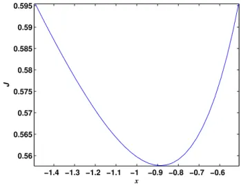
problem can be considered as a minimum square minimiza-tion problem and it is equivalent to minimize the sum of the square of power coefficients of these measurements. So, a minimization criterionJcan be designed as follows:
J=
0.67x 4.67−4x
2
+
4.67 4.67−4x
2
+
−4.67x 4.67−4x
2
(28) Study of the minimization criterion shows that it presents an absolute minimum forx≈ −0.9 as shown in Fig. 1. Eval-uating power coefficients forx= −0.9 leads to a power of −0.072 forNwterm, a power of 0.56 forZ and a power of
0.50 forKdp. It is clear that the power coefficient ofNwis
close to zero. Also, powers coefficients ofZ andKdp are
less than the unity, which traduce a powerless relation be-tweenR,Z, andKdp. Consequently, use of the found value
ofxleads to minimize both systematic error effects (through minimizingNwpower coefficient) and measurement error
ef-fects (through minimizing theZandKdppower coefficients).
4 The proposed real-like polarimetric weather radar measurements generator
In this section a “real-like” weather radar data generator us-ing the Rayleigh approximation is developed.
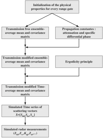
4.1 General description of the proposed simulator The proposed simulator is based on a three step approach (Ryzhkov et al., 2005). The first step consists of adopting a physical model of the rain drops which takes into account not only the Drop Size Distribution (DSD) presented in Sect. 2.1, but also the Drop Orientation Distribution. In the second
−1.4 −1.3 −1.2 −1.1 −1 −0.9 −0.8 −0.7 −0.6 0.56 0.565 0.57 0.575 0.58 0.585 0.59 0.595 x J
Fig. 1.Optimization criterion.
level, we adopt a statistical model that consider the radar rain returns as realizations of a multivariate Gaussian ran-dom variable. Finally, the outputs of the physical model are used as inputs of the statistical one according to the Ergod-icity principle in order to generate the “real-like” data. The proposed simulator is highly modular, allowing the emula-tion of a wide variety of the rain physical processes thanks to its great flexibility in fixing the starting physical properties of the rain drops and the geometrical configuration of the radar. Also, it is envisageable to implement additional modules in the simulator, such as the Mie and theT-Matrix approxima-tions and the Doppler radial winds modules. An extension of the proposed simulator to the 2-D case is published in Elm-zoughi et al. (2007).
4.2 The physical model
Besides the shape, the size distribution, and the velocity of the rain drops presented in Sect. 1, the considered physi-cal model describes the geometriphysi-cal configuration of the rain drop when the spheroid symmetry axis is oriented alongON with anglesθbandφb. The angle between the incident
direc-tionOIandONisψ.QT is the projection ofON onto the plane of polarization of the incident wave. QV is the pro-jection ofOZonto the plane of polarization of the incident wave. The canting angle is the angle measured clockwise between the line segmentsQV andQT,β=V QT\.
Initialization of the physical properties for every range gate
Transmission free ensemble-average mean and covariance
matrix
Propagation constantes : attenuation and specific
differential phase
Transmission modified ensemble-average mean and covariance
matrix
Ergodicity principle
Transmission modified Time-average mean and covariance
matrix
Simulated Time series of scattering vectors
X=[Shh,Shv,Svv]
Simulated radar measurements (Zhh,Zvv,Kdp,Zdr,...)
Fig. 2.The block diagram for the principle of the proposed data generator.
4.3 The statistical model
It is widely accepted by the meteorological community (Bringi and Chandrasekar, 2001) that the scattering vector X=(Shh,Shv,Svv), X can be modelled as having a
multi-variate complex Gaussian distribution: PX(x)=
1 π3|C|e−
xTC−1x, (29)
whereC is the complex covariance matrix, T indicates the complex conjugate, and| · |is the determinant.
4.4 Ergodicity principle and polarimetric data generation
It was shown in Bringi and Chandrasekar (2001) and Tough et al. (1995) that the radar returns from a distributed tar-get verify the ergodicity property. Thus, the time-average is equal to the ensemble average of the radar returns, and the time covariance matrix can be expressed as an
ensemble-average covariance matrix. So, considering the physical model described below, time-statistics can be ob-tained by averaging over both the DSD and the orientation distribution. From an electromagnetic point of view (Guifu et al., 2001), the scattering amplitudes of a fixed rain drop whose orientation is described by the couple (ψ,β) verify the following relations:
Shh= Afa+Bfb Shv=E(fa−fb) Svv= Cfa+Dfb
, (30)
whereA , B, C, D,andEdepend only on the orientation (ψ,β) of the drop, andfa andfb are the complex backscattering
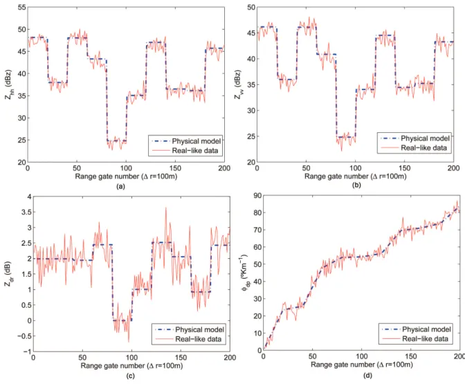
Fig. 3.Example of the generated data(a)horizontal reflectivity(b)vertical reflectivity(c)the differential reflectivity (d) differential phase shift.
analytically computed. Moreover, they can be approximated as
fa =αaDβa fb=αbDβb
, (31)
whereαa,βa,αb, andβbare adjusted following the water
ac-tivity (stimulating radar wavelength and water temperature), andD is the drop diameter. Now, let< X >=(< Shh>,< Shv>,< Svv>)be the average scattering vector. Given that ψ,βandDare independent, it is easy to prove that:
< X >=(A < fa>+B < fb>,E < fa−fb>, C < fa>+D < fb>)
, (32) where the upperline designates the averaging over orientation and<>is averaging over the (DSD). In order to take into ac-count the propagation effects, propagation constantsγh and γv can be analytically computed using the Oguchi solution
presented in Oguchi (1983). Finally,
< X >=(< Shh> e−2γhr,< Shv> e−(γh+γv)r,< Svv> e−2γvr)
. (33)
Elements of the ensemble-average covariance matrixC can be computed in the same way. Once physical statistics are computed, radar returns are generated as a limited number of realizations of a multivariate Gaussian variable following the statistical model and according to the ergodicity princi-ple. Then the covariance matrix is estimated from the gener-ated scattering vector. From the estimgener-ated covariance matrix the principal radar measurements namely the horizontal and vertical reflectivitiesZhhandZvv, the differential reflectivity Zdr and the differential phase shiftφdp from which is
esti-matedKdpare estimated. Diagram in Fig. 2 summarizes the
principle of the proposed data generator.
5 Simulation and result analysis
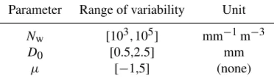
Table 1.The considered variability ranges for the drop size.
Parameter Range of variability Unit
Nw [103,105] mm−1m−3
D0 [0.5,2.5] mm
µ [−1,5] (none)
estimators are compared. Finally, a rigorous error structure analysis is performed. A dimilar simulation and result anal-ysis with a different approch is given in (Giangrande and Ryzhkov, 2008).
5.1 Validation of the proposed “real-like” polarimetric data generator
A range profile consisting of 200 range gates of depth1r= 100 m has been generated. Homogeneity has been assumed for 20 consecutive gates (by invoking the ergodicity princi-ple, the time mean and covariance matrix, of vectorX, are equal for each range gate and could be evaluated as done in the previous section given the physical properties of the drops).
The wavelength was fixed to 10 cm; the temperature to 10◦C. The distribution ofψ wasN(90◦,4◦)and the distri-bution ofβ wasN(0◦,4◦). The DSD parametersNw,D0,
and µ are fixed independently in the ranges presented in Table 1 (Ulbrich, 1983), allowing rain rates between 0 and 200 mm h−1. However, we had taken into account only usual rainfall rates in semi-arid regions. The number of samples for every range gate is 16. Starting from these physical parame-ters, “real-like” radar returns were generated from which the “real-like”Zhh,Zvv,Zdr, andφdp were deduced. Figure 3
shows the obtained results.
Figure 3a, b, c, and d represent, respectively, the horizon-tal reflectivityZhh, the vertical oneZvv, the differential
re-flectivityZdr, and the differential phase shiftφdp obtained
using the proposed simulator. These figures show that the real measurements appear as the sum of the exact physical measurements and a random noise. This noise results from the fact that the rain is a time-varying and distributed target. Indeed, we can verify that the real-like reflectivities range between 0 and 60 dBz and the differential reflectivity ranges between−1 and 4 dB, which are very well known intervals for the rain target (Bringi and Chandrasekar, 2001). Also, the reflectivities are highly correlated in accordance with results in the literature, which indicates that the correlation factor for rain targets is over 0.97. Finally, it is important to remark that the specific differential phaseKdp, which is obtained as
the slope of a local linear regression made on the differential phaseφdp, will be very noisy for small values due to the noise
resulting from the scattering differential phase. To avoid this problem, a smooth version ofφdp is used to estimate Kdp.
Consequently, results obtained by the proposed simulator be-have as real measurements and can be used as a laboratory re-alistic tool to validate and compare rain rate estimation algo-rithms. In order to keep an acceptable spatial resolution and to guarantee a good denoising ofφdp, the smoothing is
per-formed by averaging along every 5 consecutive range gates. 5.2 Rain rate estimation physically-based algorithms
comparison
In order to evaluate the performance of the adopted tech-nique, theR(Z),R(Z,Zdr),R(Kdp), andR(Kdp,Zdr)
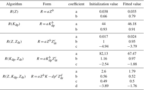
rithms have been considered for comparison. These algo-rithms follow a power law relation as shown in Table 2 (co-efficients were computed by performing non linear regres-sions). These results are roughly similar to those obtained for X-band radar by Matrosov et al. (2002). Then corre-sponding coefficients can be estimated by performing non linear regressions. The least square algorithm described in Marquardt (1963) is used for that. In order to ensure good fittings, initialization of the regression algorithm is very im-portant. Multiplicative coefficientsa, which depend on both Nw, andµ for all the algorithms, were initialized by
aver-aging over these two parameters. The power coefficients – namelyb,c, andd– were initialized to their theoretical val-ues. Simulated data is now used as input to the least square non linear algorithm. Table 2 summarizes results for fitting estimated rain rate and exact real rate. It shows initialization and fitted values of the different algorithms coefficients. Af-ter deAf-termining the parametrization coefficients, the rain rate was estimated with every algorithm using the generated radar data.
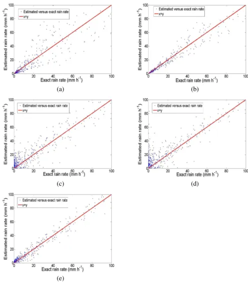
Figure 4 shows scatter plots of estimated rain rate obtained using (a)R(Z), (b)R(Z,Zdr), (c)R(Kdp), (d)R(Kdp,Zdr),
and (e) R(Z,Kdp,Zdr)versus the exact rain rate computed
from the known microphysical DSD properties. Figures 4a and 4b show thatZ-based algorithms present large deviations for rain rates over 50 mm h−1. This deviation is about 30 % for the R(Z) algorithm and about 25 % for the R(Z,Zdr)
algorithm. However, they give good results for lower rain rates. On the other hand, from Fig. 4c and d, it is clear that R(Kdp)andR(Kdp,Zdr)present very large errors for small
rain rates, though they provide good results for rain rates over 50 mm h−1 with errors under 15 %. Figure 4e presents the results corresponding to the proposed method. In this case, deviation errors are under 20 % for all rain rates.
Table 2.Initialization and fitting coefficients for the different rain rate algorithms.
Algorithm Form coefficient Initialization value Fitted value
R(Z) R=aZb a 0.038 0.035
b 0.66 0.79
R(Kdp) R=aKdpb a 44 46.18
b 0.93 0.91
a 0.017 0.024
R(Z,Zdr) R=aZbZcdr b 1 0.95
c −4.94 −3.79
a 82,13 67.47
R(Kdp,Zdr) R=aKdpbZcdr b 1.16 0.97
c −2.54 −1.88
a 2.6 1.79
R(Z,Kdp,Zdr) R=aZbK−dpcZdrd b 0.56 0.52
c 0.49 0.5
d −3.89 −1.76
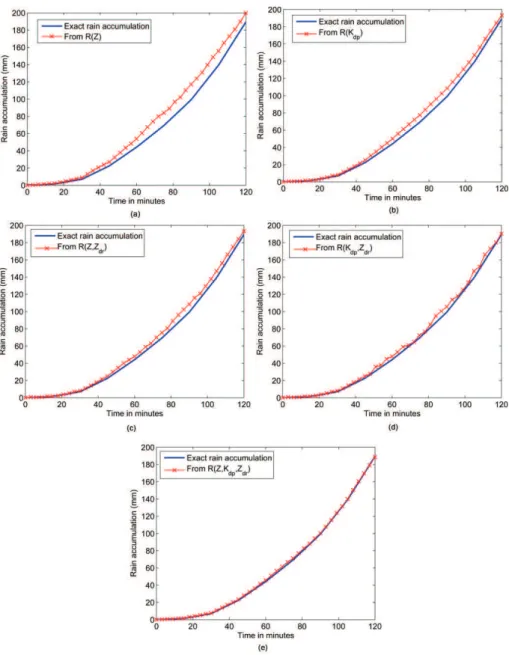
However, Fig. 5e shows that the proposed algorithm per-forms better in terms of the peak accumulation.
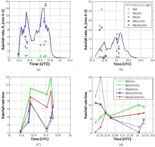
Moreover, the different given rain rate estimation algo-rithms were tested on radar data taken in light to moder-ate stratiform rainfalls with rain rmoder-ates varying between 2 and 15 mm h−1. The data were collected by Matrosov et al. (2006), using experimental DSDs that were recorded by an impact Joss-Waldvogel disdrometer (JWD) deployed at the Boulder Atmospheric Observatory (BAO) during June of 2004. Thus, we got,Z,Zdr, andKdp at S-band for
ex-perimental DSDs. The corresponding in-situ rain rates were acquired using the Colorado State University–University of Chicago Illinois State Water Survey (CSU-CHILL) radar. Two test sites were considered: the first one is located at BAO (6.5 km from the NOAA radar and 54.5 km from CSU-CHILL), and the second one at the University of Colorado’s Platteville (PLT) observatory (27.8 km from the NOAA/ESRL radar and 30.4 km from CSU-CHILL). The considered coefficients for the rain rate expressions are those published in Bringi and Chandrasekar (2001). The numerical application in this case is given in Fig. 6a and b. The empiri-cal results confirm the simulated ones. In fact, the rain rates estimated with the developed approach (based on the full set of polarimetric radar measurements) performs optimally.
The performance of the different rain rate estimation algo-rithms was quantitatively evaluated through the rainfall rate bias (computed as the absolute difference between the es-timated rainfall rate and the closest measured one in time). Figure 6c and d illustrate, respectively, rainfall rate bias over BAO and PLT for the different algorithms. It can be seen that there is a good agreement with theory. In fact, over a rainfall rate of 8 mm h−1, theKdp-based rain rate estimation
algorithm performs better than theZ-based ones. Thus, in Fig. 6d the third measured sample, corresponding at around 22:40 UTC on 17 June over PLT, is an inflection point of the bias curve, as the three next measured samples have rainfall rates over 8 mm h−1. Moreover, the optimality of theR(Z,Kdp,Zdr)algorithm is confirmed, considering both
cases of heavy and light rain. In fact, the bias red curves in Fig. 6c and d are always in the middle with respect to the bias green curves (computed for theZ−based algorithms) and the blue ones (computed for theKdp−based algorithms).
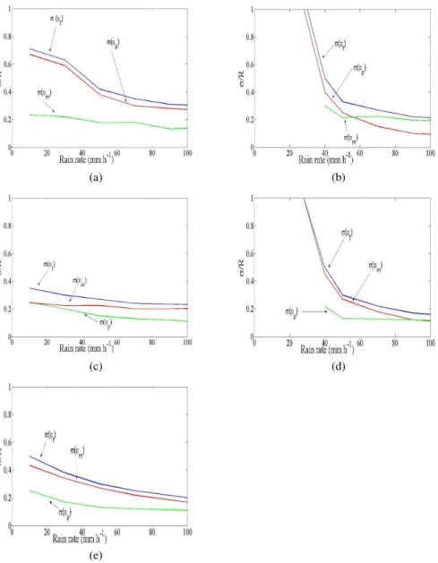
5.3 Estimation error analysis
Now, letRbbe the generic estimator from one of the five al-gorithms. Following Chandrasekar et al. (1993), the fluctu-ations of the errors in Rbregarding the rain rate R can be written as:
b
R=R+ǫp+ǫm=R+ǫt, (34)
whereǫprepresents errors due to the parametric form ofRb, ǫm represents errors due to the measurements, andǫt
repre-sents the total error. Simulations are performed in order to compute the normalized averages ofǫt, which represents the
estimation algorithms biases as well as the normalized stan-dard deviationsσ (ǫt)/R,σ (ǫp)/Randσ (ǫm)/Rfor every
(a) (b)
(c) (d)
(e)
Fig. 4.Estimated versus exact rain rate.(a)R(Z),(b)R(Z,Zdr),(c)R(Kdp),(d)R(Kdp,Zdr),(e)R(Z,Kdp,Zdr).
from simulated real-like data. Thenσ (ǫp)are computed
us-ing simulated exact (only physically-based) data, andσ (ǫm)
are deduced from:
σ (ǫm)=
q
σ2(ǫ
m)−σ2(ǫp). (35)
Figure 7 shows the biases obtained for the different algo-rithms. As expected, theKdp-based algorithms present very
high biases for low rain rates, and very low biases for high rain rates. However, theZ-based algorithms as well as the proposed one present acceptable results in both high and low rain rates.
In Bringi and Chandrasekar (2001), the expressions for relative bias error is given for the different existing rain rate estimation algorithms (R(Z), R(Z,Zdr), R(Kdp), and R(Kdp,Zdr). In order to operate an inter-comparison with the
Bringi formulas, the retrieval error for the adopted technique
is developed. Using perturbation analysis and Eq. (27) we deduct the variance ofǫmofR(Z,Kdp,Zdr)as,
var(ǫm)
R2 =b
2(x)var(Z)
Z2 +c
2(x)var(Kdp)
Kdp2 +d
2(x)var(Zdr)
Zdr2 (36) As Kdp is estimated over a path (say, L=N 1r),
the evaluation of the relative bias error of the rain rate (R(Z,Kdp,Zdr)) have to be computed for a fixed path length.
Thus, we considered the same numerical application as given by Bringi (Bringi and Chandrasekar (2001), in Sect. 8.3.3): the standard error in the measurement of reflectivity is 0.8 dB, error in the measurement ofZdr, L=3 km and 1r=
0.15 km. The variance of Z is also reduced by a fac-tor of √N. Figure 8 shows the obtained standard devia-tions, respectively, for (a)R(Z), (b)R(Z,Zdr), (c)R(Kdp),
(d)R(Kdp,Zdr), and (e)R(Z,Kdp,Zdr). Again, these plots
Fig. 5. Rain accumulation. (a)R(Z),(b)R(Kdp),(c)R(Z,Zdr),(d)R(Kdp,Zdr),(e)R(Z,Kdp,Zdr). Figure 7 Obtained biases for the
physically-based rain rate estimation algorithm.
rates. So, the proposed method presents a very interesting tradeoff, allowing good rain rate estimates simultaneously for both light and heavy rain.
6 Conclusions
A rain rate estimation algorithm adapted for regions with light and heavy rain has been presented, assuming a well cal-ibrated radar. It is based onZdr,Z, andKdpmeasurements.
A “real-like” weather radar generator has also being intro-duced. This rain signals simulator is based on both statisti-cal and physistatisti-cal modes. Thus, using the ergodicity princi-ple, it makes possible the generation of “real-like” radar data
starting from fixed physical properties of the drops. Sim-ulations made with generated data show that the proposed one performs well for both light and heavy rain rates com-pared to other algorithms. These results were also validated through in-situ data. The data were collected by Matrosov et al. (2006), using experimental DSDs that were recorded by an impact Joss-Waldvogel disdrometer (JWD) deployed at the Boulder Atmospheric Observatory (BAO) during June of 2004. Thus, we gotZ,Zdr, andKdpat S-band for
(a) (b)
(C) (d)
Fig. 6.Rain rates for light to moderate rainfalls over(a)BAO and(b)PLT on 17 June 2004 and, respectively, their corresponding rainfall
rate bias(c)for BAO and(d)for PLT.
0 50 100 150 200 250 300 350
0 2 4 6 8 10 12
Rain rate
bias (%)
R(Z,K
dp,Zdr)
R(K
dp,Zdr)
R(Kdp)
R(Z,Zdr)
R(Z)
Fig. 7.The estimator bias versus the rain rate.
from the NOAA radar and 54.5 km from CSU-CHILL), and the the second one at the University of Colorado’s Platteville (PLT) observatory (27.8 km from the NOAA/ESRL radar and 30.4 km from CSU-CHILL).
Appendix A
Covariance matrix elements computations
The model supposes thatψandβ are independent and fol-low, respectively, N(ψ0,σψ) and N(β0,σβ). This means that the rain target verifies a reflection symmetry around the axis defined by the couple of angles (ψ0,β0). In these
con-ditions, the off-diagonal covariance matrix are zeros and the remaining elements are given by:
<|Shh|2> =< (Afa+Bfb)(Afa+Bfb)∗>
=A2<|fa|2>+AB(< f
afb∗>+< fa∗fb>)+ B2<|f
b|2>
<|Svv|2> =< (Cfa+Dfb)(Cfa+Dfb)∗>
=C2<|fa|2>
+CD(< fafb∗>+< fa∗fb>)+ D2<|fb|2>
<|Svh|2> =< (E(fb−fa))(E(fb−fa))∗>
=E2<|f
b−fa|2>
< ShhS∗vv>=< (Afa+Bfb)(Cfa+Dfb)∗>
=AC <|fa|2>+AD < fafb∗>+BC < fa∗fb>+ BD <|fb|2>
(A1)
(a) (b)
(c) (d)
(e)
Fig. 8.Standard deviations, considered from Bringi and Chandrasekar (2001)(a)R(Z),(b)R(Kdp),(c)R(Z,Zdr),(d)R(Kdp,Zdr), and for
the proposed algorithm(e)R(Z,Kdp,Zdr).
that it was assumed that orientation and particle size distri-butions are independents. The model supposes thatψ and β are independent and follow, respectively,N(ψ0,σψ)and N(β0,σβ). So, the values ofA2,AB, AC, AD, B2, BC, BD,C2,CD, andD2can be easily evaluated using the
fol-lowing relationships: R+∞
−∞sin2(x)
1
√
2π σxe
−(x−x0)2 2σx2
dx =12(1−e−2σx2cos(2x0))
R+∞ −∞cos2(x)
1
√
2π σxe
−(x−x0)2
2σx2 dx=12(1+e−2σ2
xcos(2x0))
R+∞ −∞sin
4(x)√1 2π σxe
−(x−x0)2
2σx2 dx =38+e8σ
2 xcos(4x0)
8 −
e−2σx2cos(2x0)
2 R+∞
−∞cos4(x)√21π σxe
−(x−x0)2 2σ2
x dx=38+e8σ
2 xcos(4x0)
8 +
e−2σx2cos(2x0)
2
(A2)
If we suppose that: fa =α1Dβ1
fb=α2Dβ2 (A3)
we have:
< fafb>=< α1Dβ1α2Dβ2>
=R0+∞α1Dβ1α2Dβ2N0Dµe(−3D)dD
=N0α1α2R0+∞D(β1+β2+µ)e(−3D)dD
=N0α1α2R0+∞3−(β1+β2+µ+1)D(β1+β2+µ)e−DdD
=N0α1α23−(β1+β2+µ+1)R0+∞D(β1+β2+µ+1)−1e−DdD
=N0α1α23−(β1+β2+µ+1)Ŵ(β1+β2+µ+1)
(A4)
Given thatfaandfbare real then it follows:
<|fa|2>=< fafa> =N0α213−(2β1+µ+1)Ŵ(2β1+µ+1)
Acknowledgements. The authors would like to thank Sergey Matrosov and Robert Cifelli for their time and their support in offering and explaining the data collected as part of the GPM pilot experiment. They also gratefully acknowledge the spanish Ministry of Science and Innovation for partially funding this research under project TEC2008-06736-C03-02.
Edited by: A. Mugnai
Reviewed by: two anonymous referees
References
Atlas, D.: Advances in radar meteorology, Advances in
Geo-physics, Landsberg and Mieghem, Eds, New York, Academic Press, 317–478, 1964.
Atlas, D.: Early foundations of the measurement of rainfall by radar, Radar in Meteorolog. D. Atlas, ED., American Meteoro-logical society, Boston, J. Appl. Meteor., 86–97, 1990.
Atlas, D. and Ulbrich, C. W.: Path and area integrated rainfall measurement by microwave attenuation in 1-3 cm band, J. Appl. Meteor., 16, 1322–1331, 1977.
Atlas, D., Srivastava, R. C., and Shekhon, R. S.: Dopler radar char-acteristics of precipitation at vertical incidence, Rev. Geophys. Space Phys., 2, 1–35, 1973.
Beard, K. V. and Chuang, C. A new model for the equilibrium shape of raindrops, J. Atmos. Sci., 44, 1509–1524, 1987. Beaver, J. and Bringi, V. N.: The application of the S-band
polari-metric radar measurements to Ka band attenuation prediction, Proc. IEEE, 134, 431–437, 1997.
Bringi, V. N. and Chandrasekar, V.: Polarimetric Doppler Weather Radar, Principles and Applications, 1st Edn., Cambridge, UK, Cambridge Univ. Press, 2001.
Brandes, E. A., Ryzhkov, A. V. and Zrnic, D. S.: An evaluation of radar rainfall estimates from specific differential phase, J. Atmos. Oceanic Technol., 18, 363–375, 2001.
Bringi, V. N., Chandrasekar, V., and Xiao, R.: Raindrop axis ra-tio and size distribura-tions in Florida rainshafts: An assessment of multiparameter radar algorithms, IEEE Trans. Geosci. Remote Sens., 36, 703–715, 1998.
Chandrasekar, V., Cooper, W. A., and Bringi, V. N.: Axis ratios and oscillation of raindrops, J. Atmos. Sci., 45, 1325–1333, 1988. Chandrasekar, V., Gorgucci, E., and Scachilli, G.: Optimization of
multiparameter radar estimates of rainfall, J. Appl. Meteor., 12, 1288–1293, 1993.
Doviak, R. J. and Zrnic, D. S.: Doppler Radar Weather Observa-tions, Academic Press, New York, 1993.
Elmzoughi, A., Abdelfattah, R., Belhadj, Z., and Santalla Del Rio, V.: 2D weather radar data simulator using specific reflectivitie and phase measurements for the rain rate estimation algorithms validation, European Signal Processing Conference (EUSIPCO 2007), 1663–1666, 2007.
Giangrande, S. E. and Ryzhkov, A. V.: Estimation of Rainfall Based on the Results of Polarimetric Echo Classification., J. Appl. Meteorol. Climatol., 47, 2445–2462, 2008.
Green, A. W.: An approximation for the shapes of large raindrops, J. Appl. Meteor., 14, 1578–1583, 1975.
Guifu, Z., Vivekanandan, J., and Brandes, E.: A Method For Es-timating Rain Rate And Drop Size Distribution From Polarimet-ric Radar Measurements IEEE Trans. Geosci. Remote Sens., 39, 830–841, 2001.
Laws, J. O. and Parsons, D. A.: The relationship of raindrop size to intensity, Trans. Amer. Geophys. Union, 24, 452–460, 1943. Marquardt, D.: An Algorithm for Least Squares Estimation of
Non-linear Parameters, SIAM J. Appl. Math, 11, 431–441, 1963. Marshall, J. S. and Palmer, W.: The distribution of raindrops with
size, J. Meteor., 5, 165–166, 1948.
Matrosov, S. Y., Clark, A. K., Martner, B. E. and Tokay, A.: X-band polarimetric radar measurements of rainfall, J. Appl. Meteorol., 41, 941–952, 2002.
Matrosov, S. Y., Cifelli, R., Kennedy, P. C., Nesbitt, S. W., Rutledge, S. A., Bringi V. N., and Martner B. E.: A Comparative Study of Rainfall Retrievals Based on Specific Differential Phase Shifts at X- and S-Band Radar Frequencies, J. Atmos. Ocean. Tech., 23, 952–963, 2006.
McCormick, G. C. and Hendry, A.: Techniques for the determi-nation of the polarization properties of precipitation, Radio Sci., 14, 1027–1040, 1979.
Oguchi, T.: Electromagnetic wave propagation and scattering in rain and other hyrdrometeors, IEEE. Proc., 71, 1029–1078, 1983. Pruppacher, H. R. and Beard, K. V.: A wind tunnel investigation of the internal circulation and shape of water drops falling at termi-nal velocity in air, Meteor. Soc., 96, 247–256, 1970.
Ryzhkov, A. V., Giangrande, S. E., and Schuur, T. J.: Rainfall Estimation with a Polarimetric Prototype of WSR-88D, J. Appl. Meteorol., 44, 502–515, 2005.
Sachidananda, M. and Zrnic, D. S.: Rain rate estimates from dif-ferential polarization measurements, J. Atmos. Ocean. Technol., 4, 588–598, 1987.
Seliga, T. A. and Bringi, V. N.: Potential use of radar differential reflectivity measurements at orthogonal polarization for measur-ing precipitation, J. Appl. Meteor., 15, 69–76, 1976.
Tough, R. J. A., Blacknell, D., and Quegan, S.: A Statistical De-scription of Polarimetric Synthetic Aperture Radad Data, Proc. Roy. Soc., 449, 567–589, 1995.